Sage Journals: Discover world-class research

Abstract

We develop a multi-dimensional numerical differentiation method in this paper. To obtain stable numerical derivatives, the Tikhonov regularization method in Hilbert scales is proposed to deal with illposedness of the problem. The penalty term in Tikhonov functional is more general so that we can choose the regularization parameter without the smoothness parameter and the a priori bound of exact solution. Numerical examples are also presented to check the effectiveness of the method.

Keywords

Numerical differentiation ill-posed problem Tikhonov regularization method Hilbert scales

Introduction

Numerical differentiation is a problem of determining the derivatives of a function from its perturbed values. It is well known to be ill posed in the sense that every small error in the measurement may cause huge errors in the computed derivatives. It arises from many processes of scientific researches and applications, e.g. the identification of the discontinuous points in an image process,^1,2 Volterra integral equation,^3,4 identification,⁵ etc. A number of techniques have been well developed for numerical differentiation in one-dimensional case,^{6,7,8,9,10–14,15,16} but so far only a very few results on the high dimensional cases have been reported.^17,18,19,20 In the literatures,^8,12,13 the finite difference method has been proposed. The stepsize is used as a regularization parameter for noisy data. So the specified points cannot be too dense, which hinders the application of the methods. In the literatures,^7,10,11 the Fourier method has been used to solve the numerical differentiation problem. The regularization parameter is a priori in these methods. It is well known that the ill-posed problem is usually sensitive to the regularization parameter and the a priori bound is usually difficult to be obtained precisely in practice.

In the literatures,^19,20 the Tikhonov regularization method has been considered to deal with the numerical differentiation problem. In this paper, we will use the method of Tikhonov regularization in Hilbert scales to solve the problem. We will show that the regularization parameter can be chosen by a discrepancy principle in Hilbert scales which is proposed by Neubauer.²¹ The smoothness parameter and the a priori bound of exact solution are not needed for the new method.

This paper is organized as follows. In the next section, the method to construct approximate function from the noise data is proposed. The convergence results with corresponding regularization parameter choice rules will be found in The choices of regularization parameter β and convergence results section. Some numerical results are given in the Numerical examples section to show the effectiveness of the new method.

Definition of approximate function

Let $x = (x 1, x 2, \dots, x d) \in ℝ d$ and $\overset{\land}{h}$ denote the Fourier transform of $h \in L 2 (ℝ d)$ defined by

\overset{\land}{h} (ξ) = F [h (x)] = \frac{1}{\sqrt{2 π}} \int ℝ d h (x) e - i ξ \cdot x d x

(1) where

ξ = (ξ 1, ξ 2 \dots, ξ d)

and

ξ \cdot x = \sum_{k = 1}^{d} ξ k x k

, and

| | \cdot | | p

denotes the norm in Sobolev space

H p (ℝ)

defined by

| | h | | p : = (\int ℝ d (1 + | ξ | 2) p | \overset{\land}{h} (ξ) | 2 d ξ) 1 / 2

(2)

When p = 0, $| | \cdot | | 0 = : | | \cdot | |$ denotes the $L 2 (ℝ)$ norm. Next, let $ℕ$ be the set of all non-negative integers. For any d tuple $α = (α 1, α 2, \dots, α d) \in ℕ d, | α | = \sum_{l = 1}^{d} α l$ . The notation ∂_j stands for $\frac{\partial}{\partial x j}$ , the symbol $D α v = \partial x 1 α 1 \partial x 2 α 2 \dots \partial x d α d v$ .

Our problem is to determine derivatives $D α g, | α | \leq p$ of a function $g \in H p (ℝ d)$ from its perturbed data g^δ. We assume that the exact and measured data satisfy

‖ g - g δ ‖ \leq δ

(3)

From the theories of Fourier transform

D α g = F - 1 ((- i) | α | Π_{k = 1}^{d} ξ_{k}^{α k} \cdot \overset{\land}{g})

(4)

It is apparent that the exact data $\overset{\land}{g}$ must decay faster than the rate $| ξ | - | α |$ . However, the measured function g^δ does not possess such a decay property in general. So

F - 1 ((- i) | α | Π_{k = 1}^{d} ξ_{k}^{α k} \cdot \overset{\land}{g} δ)

(5) cannot give a reliable approximation for D^αg. In the following, we apply the Tikhonov regularization method to reconstruct a new function

ϕ δ

from the perturbed data g^δ.

D α ϕ δ

will give a reliable approximation of D^αg. Before doing that, we impose an a priori bound on the exact data g

‖ g ‖ p \leq E, p > 0

(6) where E > 0 is a constant.

Let $ϕ δ = ϕ β, δ$ be the minimizer of the Tikhonov functional

Φ (ϕ) = ‖ ϕ - g δ ‖ 2 + β ‖ ϕ ‖ q 2

(7) where β > 0 is a regularization parameter and q is a positive real number. The function

(1 + | ξ | 2) - q

is going to occur throughout this paper and will be denoted by

λ (ξ)

. It can be verified that

ϕ β, δ

is the solution of the following equation

(I + β F - 1 (1 + | ξ | 2) q F) ϕ = g δ

(8)

So we can get

\overset{\land}{ϕ} β, δ = \frac{1}{1 + β (1 + | ξ | 2) q} \overset{\land}{g} δ

(9)

That is to say

ϕ β, δ = F - 1 [\frac{1}{1 + β (1 + | ξ | 2) q} \overset{\land}{g} δ]

(10)

By $ϕ β, δ$ , we can give an approximation of D^αg as follows

D α ϕ β, δ = F - 1 [\frac{(- i) | a | Π_{k = 1}^{d} ξ_{k}^{α k}}{1 + β (1 + | ξ | 2) q} \overset{\land}{g} δ]

(11)

Lemma 1. For $0 \leq b \leq 1$ , we have

sup λ \geq 0 \frac{λ b}{λ + β} = b b (1 - b) 1 - b β b - 1

(12)

Lemma 2.

‖ D α (ϕ β, δ - ϕ β) ‖ = O (δ \cdot β - | α | / 2 q)

(13) where

ϕ β

is the unique minimizer of (7) with g instead of g^δ.

Proof. Due to Parseval formula

‖ D α (ϕ β, δ - ϕ β) ‖ 2 = \int ℝ d | \frac{(- i) | α | Π_{k = 1}^{d} ξ_{k}^{α k}}{1 + β (1 + | ξ | 2) q} (\overset{\land}{g} δ - \overset{\land}{g}) | 2 d ξ \leq \int ℝ d | \frac{| ξ | | α |}{1 + β (1 + | ξ | 2) q} (\overset{\land}{g} δ - \overset{\land}{g}) | 2 d ξ \leq \int ℝ d | \frac{(1 + | ξ | 2) \frac{| α |}{2}}{1 + β (1 + | ξ | 2) q} (\overset{\land}{g} δ - \overset{\land}{g}) | 2 d ξ \leq (sup λ \geq 0 \frac{λ (ξ) \frac{2 q - | α |}{2 q}}{λ (ξ) + β}) 2 \int ℝ d | \overset{\land}{g} δ - \overset{\land}{g} | 2 d ξ

(14)

The proposition follows by applying (12) with b replaced by $\frac{2 q - | α |}{2 q}$ .

Lemma 3. If $g \in H p (ℝ d)$

‖ D α (ϕ β - g) ‖ \leq c β \cdot β \frac{p - | α |}{2 q}

(15) where c_β is defined by

c_{β}^{2} : = \int ℝ d \frac{β 2 - u λ (ξ) u}{(λ (ξ) + β) 2} (1 + | ξ | 2) p | \overset{\land}{g} | 2 d ξ, u : = \frac{p - | α |}{q}

(16)

Proof. With the representation

ϕ β = F - 1 [\frac{1}{1 + β (1 + | ξ | 2) q} \overset{\land}{g} (ξ)]

(17) we have

‖ D α (ϕ β - g) ‖ 2 = \int ℝ d | \frac{(- i) | α | Π_{k = 1}^{d} ξ_{k}^{α k} β (1 + | ξ | 2) q}{1 + β (1 + | ξ | 2) q} \overset{\land}{g} (ξ) | 2 d ξ = \int ℝ d | \frac{(- i) | α | Π_{k = 1}^{d} ξ_{k}^{α k} β (1 + | ξ | 2) q - \frac{p}{2}}{1 + β (1 + | ξ | 2) q} \times (1 + | ξ | 2) \frac{p}{2} \overset{\land}{g} (ξ) | 2 d ξ \leq \int ℝ d (\frac{β (1 + | ξ | 2) q + \frac{| α |}{2} - \frac{p}{2}}{1 + β (1 + | ξ | 2) q}) 2 (1 + | ξ | 2) p | \overset{\land}{g} | 2 d ξ = \int ℝ d \frac{β 2 (1 + | ξ | 2) | α | - p}{[(1 + | ξ | 2) - q + β] 2} (1 + | ξ | 2) p | \overset{\land}{g} | 2 d ξ \leq β u \int ℝ d \frac{β 2 - u λ (ξ) u}{(λ (ξ) + β) 2} (1 + | ξ | 2) p | \overset{\land}{g} | 2 d ξ

(18)

The choices of regularization parameter β and convergence results

For any $w \in L 2 (ℝ d)$ , we define

d (β, w) : = \int ℝ d (\frac{β}{λ (ξ) + β}) 2 | \overset{\land}{w} (ξ) | 2 d ξ

(19)

It is apparent that the function $β \to d (β, w)$ is continuous and strictly increasing on $(0, \infty)$ and

lim β \to 0 d (β, w) = 0, lim β \to \infty d (β, w) = ‖ w ‖ 2

(20)

So we can get the following lemma

Lemma 4. Let g, g^δ satisfy (3) and

‖ g δ ‖ 2 \geq τ δ 2

(21)

for some τ > 1. Then there is a unique β > 0 such that

d (β, g δ) = τ \cdot δ 2

(22)

In the following, we denote the unique β determined in (22) by $\bar{β}$ . In the next lemma, we consider the behavior of $\bar{β}$ .

Lemma 5. Let g, g^δ satisfy (3) and (21) for a τ > 1, then

d (\bar{β}, g) = O (δ 2)

(23)

\bar{β} = O (δ \frac{2 q}{p} \cdot \bar{β} \cdot \frac{2 q}{p})

(24) where

d_{\bar{β}}^{2} = \int_{- \infty}^{\infty} \frac{\bar{β} 2 - \frac{p}{q} (1 + | ξ | 2) - p}{[λ (ξ) + \bar{β}] 2} | \overset{\land}{g} (ξ) | 2 d ξ

(25)

Proof.

Let

Lw = F - 1 (\frac{\bar{β}}{λ (ξ) + \bar{β}} \overset{\land}{w} (ξ))

(26) then

d (\bar{β}, g) = ‖ Lg ‖ 2 \leq (‖ L (g - g δ) ‖ + ‖ Lg δ ‖) 2 \leq (δ + \sqrt{C} δ) 2 = (1 + \sqrt{C}) 2 δ 2

(27)

d (\bar{β}, g) = \int ℝ d (\frac{\bar{β}}{λ (ξ) + \bar{β}}) 2 | \overset{\land}{g} (ξ) | 2 d ξ = \int ℝ d \frac{\bar{β} 2 (1 + | ξ | 2) - p}{(λ (ξ) + \bar{β}) 2} (1 + | ξ | 2) p | \overset{\land}{g} (ξ) | 2 d ξ = \int ℝ d \frac{\bar{β} 2 λ (ξ) \frac{p}{q}}{[λ (ξ) + \bar{β}] 2} (1 + | ξ | 2) p | \overset{\land}{g} (ξ) | 2 d ξ = \bar{β} \frac{p}{q} \int ℝ d \frac{\bar{β} 2 - \frac{p}{q} λ (ξ) \frac{p}{q}}{[λ (ξ) + \bar{β}] 2} (1 + | ξ | 2) p | \overset{\land}{g} (ξ) | 2 d ξ

(28)

The rest follows from a).

Now we can prove the main result of this paper.

Theorem 6. Let g, g^δ satisfy (3) and (21) for $τ > 1, s \in ℝ$ . $f \bar{α}, δ$ is defined by (11) and (22), then

‖ D α (ϕ \bar{β}, δ - g) ‖ = {O (δ \frac{p - | α |}{p}) if p < 2 q, O (δ \frac{p - | α |}{p}) if p = 2 q

(29)

Proof. With Lemma 2, Lemma 3, and Lemma 5, we obtain

‖ D α (ϕ \bar{β}, δ - g) ‖ \leq ‖ D α (ϕ \bar{β} - g) ‖ + ‖ D α (ϕ \bar{β}, δ - ϕ \bar{β}) ‖ = O (δ \cdot \bar{β} - | α | / 2 q) + c \bar{β} \cdot \bar{β} \frac{p - | α |}{2 q} = O [δ \frac{p - | α |}{p} (d_{\bar{β}}^{\frac{| α |}{p}} + c \bar{β} d_{\bar{β}}^{\frac{| α | - p}{p}})]

(30)

Using the Hölder inequality equations (16) and (25), we get

c_{β}^{2} = \int ℝ d \frac{β 2 - u λ (ξ) u}{(λ (ξ) + β) 2} (1 + | ξ | 2) p | \overset{\land}{g} | 2 d ξ = \int ℝ d [\frac{β 2 - \frac{p}{q} λ (ξ) \frac{p}{q}}{(λ (ξ) + β) 2} | \overset{\land}{g} (ξ) | 2] \frac{p - | α |}{p} [(\frac{β}{λ (ξ) + β}) 2 (1 + | ξ | 2) p | \overset{\land}{g} (ξ) | 2] \frac{| α |}{p} d ξ \leq (d_{α}^{2}) \frac{p - | α |}{p} \cdot [\int ℝ d (\frac{β}{λ (ξ) + β}) 2 (1 + | ξ | 2) p | \overset{\land}{g} (ξ) | 2 d ξ] \frac{| α |}{p}

(31)

Combining equations (30) and (31), we obtain

‖ D α (ϕ \bar{β}, δ - g) ‖ = O [δ \frac{p - | α |}{p} (d_{\bar{β}}^{\frac{| α |}{p}} + e_{\bar{β}}^{\frac{| α |}{p}})]

(32) where e_β is defined by

e_{β}^{2} = \int ℝ d (\frac{β}{λ (ξ) + β}) 2 (1 + | ξ | 2) p | \overset{\land}{g} (ξ) | 2 d ξ

(33)

Since $\bar{β} \to 0$ for $δ \to 0$ and

The theorem is proved.

Remark 7. It is obvious that if $g \in H p (ℝ)$ holds for some p > 2q, then we have

‖ D α (ϕ \bar{β}, δ - g) ‖ = O (δ \frac{2 q - | α |}{2 q})

(35)

Numerical examples

In this section, we give some numerical tests to verify the effectiveness of the new method. All examples are computed by using Matlab with τ = 1.01.

One-dimensional case

Let $Ω = [- 3, 3]$ and $x i = - 3 + ih, i = 0, 1, \dots, N - 1, h = \frac{6}{N}, N = 4096$ . The perturbed data are given by

g δ (x j) = g (x j) + j

(36) where

{j}_{j = 0}^{N}

are generated by Function

randn (N, 1) \times δ 1

in Matlab.

Example 1 First we consider the function

g (x) = e - x 2 \sin 2 π x

It is obvious that

g \in H p (ℝ)

for any

p \in ℝ

. We will give the numerical results for q = 2, 4, 8, 16, which are displayed in Table 1. We can see that when δ₁ decreases from 0.1 to 0.001, the relative errors become smaller and when q increases, the rates of convergence become larger.

Table 1.

Numerical results of Example 1.

	Relative errors of the 1st-order derivative				Relative errors of the 2nd-order derivative
δ ₁	p = 2	p = 4	p = 8	p = 16	p = 2	p = 4	p = 8	p = 16
1e-1	3.38e-02	2.46e-02	2.29e-02	2.17e-02	6.83e-02	3.13e-02	3.04e-02	3.03e-02
1e-2	5.74e-03	3.04e-03	2.36e-03	1.99e-03	2.28e-02	4.65e-03	3.23e-03	2.96e-03
1e-3	1.12e-03	3.95e-04	2.52e-04	1.88e-04	8.40e-03	7.94e-04	3.64e-04	2.99e-04

In Figure 1, we observe that the reconstructed k-th derivatives are very similar to those of the corresponding functions.

Figure 1.

Results of Example 1.

Figure 2.

Results of Example 2.

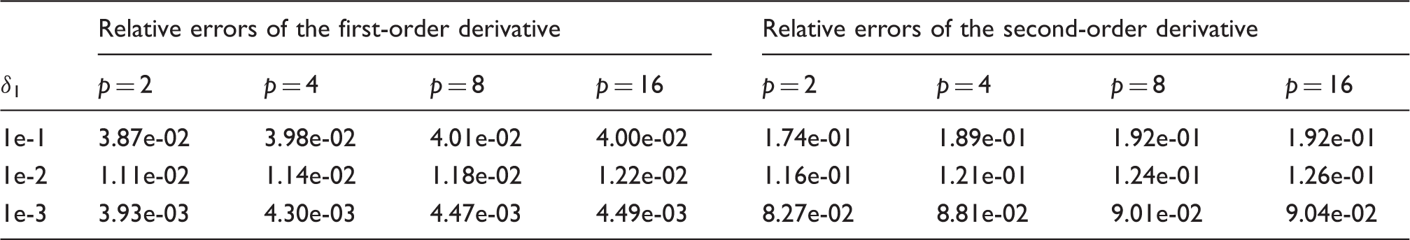
Example 2 Consider a function

g (x) = {\cos (π x) - 1, - 2 \leq x \leq 2, 0 otherwise .

In this example, we only have

g \in H 2 (ℝ)

, while we also compute with p = 2, 4, 8, 16. The results are given in Table 2, and we can see that the results are close for different p, which indicate that the method can work well even if p is greater than the smooth scale of g.

Table 2.

Numerical results of Example 2.

	Relative errors of the first-order derivative				Relative errors of the second-order derivative
δ ₁	p = 2	p = 4	p = 8	p = 16	p = 2	p = 4	p = 8	p = 16
1e-1	3.87e-02	3.98e-02	4.01e-02	4.00e-02	1.74e-01	1.89e-01	1.92e-01	1.92e-01
1e-2	1.11e-02	1.14e-02	1.18e-02	1.22e-02	1.16e-01	1.21e-01	1.24e-01	1.26e-01
1e-3	3.93e-03	4.30e-03	4.47e-03	4.49e-03	8.27e-02	8.81e-02	9.01e-02	9.04e-02

Two-dimensional case

Let $Ω = [- 4, 4] \times [- 4, 4]$ and $x i = (- 4 + i 1 h, - 4 + i 2 h), i 1, i 2 = 0, 1, \dots, N - 1, N = 256$ , The perturbed data are given by

g δ (x i) = g (x i) + i

(37) where

ɛ i

is generated by Function

randn (N) \times δ 1

in Matlab.

Example 3 We consider the function

g (x) = \sin (π x 1) \sin (π x 2) \exp (- x_{1}^{2} - x_{2}^{2})

$g \in H p (Ω)$ for any $p \in ℝ$ . We will give the numerical results for p = 8. Let $D k = \sum_{| α | = k} D α$ , and we compare D_kg and $D k ϕ β 2, δ$ for k = 1, 2, 3 in Figures 3 –5. It can be observed that the approximation derivatives match well with the exact ones.

Figure 3.

Results of Example 3: comparison of D₁g and $D 1 ϕ β 2, δ, δ = 0.01$ .

Figure 4.

Results of Example 3: comparison of D₂g and $D 2 ϕ β 2, δ, δ = 0.01$ .

Figure 5.

Results of Example 3: comparison of D₃g and $D 3 ϕ β 2, δ, δ = 0.01$ .

Conclusion

In this paper, we apply the Tikhonov regularization with a different regularization functional to reconstruct numerical derivatives. The convergence rates for approximating the derivatives are obtained when we choose the regularization parameter with a discrepancy principle. The a priori information of the exact solution is not needed and the convergence rates are self-adaptive. The method can calculate the derivatives of a function in any finite dimension space. All examples show that the proposed schemes are effective and stable.

Wan

Wang

Yamamoto

. Detection of irregular points by regularization in numerical differentiation and application to edge detection. Inverse Probl 2006; 22: 1089–1103.

Cheng J, Hon Y and Wang Y. A numerical method for the discontinuous solutions of Abel integral equations. In: Inverse problems and spectral theory: proceedings of the workshop on spectral theory of differential operators and inverse problems, Kyoto, Japan, 28 October–1 November 2002.

Gorenflo

Vessella

. Abel integral equations. Lecture Notes in Mathematics 1991; Vol 1461, Berlin: Springer.

Hanke

Scherzer

. Error analysis of an equation error method for the identification of the diffusion coefficient in a quasi-linear parabolic differential equation. SIAM J Appl Math 1999; 59: 1012–1027.

Cullum

. Numerical differentiation and regularization. SIAM J Numer Anal 1971; 8: 254–265.

Feng

Qian

. Wavelets and high order numerical differentiation. Appl Math Model 2010; 34: 3008–3021.

Groetsch

. Differentiation of approximately specified functions. Amer Math Monthly 1991; 98: 850.

Hanke

Scherzer

. Inverse problems light: numerical differentiation. Amer. Math. Monthly 2001; 108: 512–521.

10.

Qian

Feng

. A modified method for high order numerical derivatives. Appl Math Computat 2006; 182: 1191–1200.

11.

Qian

Xiong

. Fourier truncation method for high order numerical derivatives. Appl Math Computat 2006; 181: 940–948.

12.

. A new approach to numerical differentiation and integration. Math Comput Model 1996; 24: 55–68.

13.

Ramm

Smirnova

. On stable numerical differentiation. Math Comp 2001; 70: 1131–1153.

14.

Rivlin

. Optimally stable Lagrangian numerical differentiation. SIAM J Numer Anal 1975; 12: 712–725.

. A numerical differentiation method and its application to reconstruction of discontinuity. Inverse Probl 2002; 18: 1461–1476.

16.

Zhao

Meng

. A new approach to numerical differentiation. J Comput Appl Math 2009; 232: 227–239.

17.

Anderssen

Hegland

. For numerical differentiation, dimensionality can be a blessing!. Math Comp 1999; 68: 1121–1141.

18.

Bozzini

Rossini

. Numerical differentiation of 2D functions from noisy data. Comput Math Appl 2003; 45: 309–327.

19.

Wei

Hon

. Numerical differentiation by radial basis functions approximation. Adv Comput Math 2007; 27: 247–272.

. Reconstruction of numerical derivatives for scattered noisy data. Inverse Probl 2005; 21: 657–672.

21.

Neubauer

. An a posteriori parameter choice for Tikhonov regularization in Hilbert scales leading to optimal convergence rates. SIAM J Numer Anal 1988; 25: 1313–1326.

22.

Natterer

. Error bounds for Tikhonov regularization in Hilbert scales. Applicable Anal 1984; 18: 29–37.

A stabilized algorithm for multi-dimensional numerical differentiation

Abstract

Keywords

Introduction

Definition of approximate function

The choices of regularization parameter β and convergence results

Numerical examples

One-dimensional case

Two-dimensional case

Conclusion

Footnotes

Declaration of conflicting interests

Funding

References