
Abstract
This article presents anomaly detection algorithms for marine robots based on their trajectories under the influence of unknown ocean flow. A learning algorithm identifies the flow field and estimates the through-water speed of a marine robot. By comparing the through-water speed with a nominal speed range, the algorithm is able to detect anomalies causing unusual speed changes. The identified ocean flow field is used to eliminate false alarms, where an abnormal trajectory may be caused by unexpected flow. The convergence of the algorithms is justified through the theory of adaptive control. The proposed strategy is robust to speed constraints and inaccurate flow modeling. Experimental results are collected on an indoor testbed formed by the Georgia Tech Miniature Autonomous Blimp and Georgia Tech Wind Measuring Robot, while simulation study is performed for ocean flow field. Data collected in both studies confirm the effectiveness of the algorithms in identifying the through-water speed and the detection of speed anomalies while avoiding false alarms.
Keywords
Introduction
Anomaly detection for marine robots is an important practical problem because marine robots are often used in distant and hostile environments such as the deep sea and the polar oceans. During long-range or long-period missions, marine creatures and biofouling may harm robot sensors and thrusters. 1 Monitoring sensors have been installed to evaluate components vulnerable to faults. 2 For example, damaged propellers impair propulsive efficiency to control vehicle speed. These faults could be detected with rotational speed sensors installed at the propellers; however, this approach requires increased hardware complexity and cost, 3 and it may not detect unexpected external disturbances (e.g. white shark attack).
We propose anomaly detection algorithms for marine robots based on their trajectory data. Given a trajectory, we develop a learning algorithm that estimates the through-water speed of the robot as well as the ambient flow velocity. The robot speed estimate is then used to determine whether or not robot motion is abnormal. Anomaly occurs when the robot speed estimate is out of the range in normal operation. This approach complements the existing methods that detect faults of individual components based on sensor measurements. The use of trajectory data in our work follows similar motivations as previous works in surveillance applications (e.g. see the literature 4 ). Our work uses underwater trajectory data of marine robots while the previous work 5,6 uses car trajectory data and surface trajectory data of marine vessels. The major difference is the type of speed information used for anomaly detection; the former is through-water speed and the latter is ground speed.
Related work
Recent studies on ground and marine robots proposed approaches to identify abnormal robot motion. 7,8 An anomaly or fault is defined as an unacceptable deviation of at least one characteristic property of a variable from an acceptable behavior. 9 We assume that normal behaviors occur far more frequently than abnormal behaviors for the data collected. If this assumption is not true, then such techniques can produce incorrect detection results or false alarms. 10
For marine robots, most fault detection algorithms have been dealing with abnormal behaviors of the system components that are the most vulnerable to faults. 11 –13 Blocked propellers, leaking thrusters, and rotor failure are documented as frequently occurring faults. 14 In 2015, a software configuration error in an underwater glider disabled an internal mass shifter that adjusts the vehicle’s trim, leading the vehicle to sink to the seafloor and resulting in a temporary loss. 8 Instead of detecting faults in an individual component, robot motion can be used for anomaly detection. Raanan et al. 15 use a threshold technique to prevent an underwater glider from hitting the seafloor. The deviation from expected robot motion in the vertical plane is detected by monitoring stern plane angle, pitch angle, and depth rate.
Serious performance degradation can result when ocean flow speed is comparable to or exceeds the maximum through-water speed of marine robots, as is the case for underwater gliders. 16 However, the abnormal motion caused by ocean flow should not be misclassified as an anomaly for the marine robot. Therefore, it is important to identify the ambient ocean flow while estimating the through-water speed. Measuring through-water speed of marine robots is substantially difficult because of limited hardware capability. The inertial measurement unit (IMU) and the Doppler velocity log (DVL) can be combined to measure through-water speed. 17 IMU error can be corrected by the DVL, which measures both vehicle velocity with respect to ground (bottom-tracking) and flow velocity with respect to the vehicle (water-tracking). 18 However, DVL accuracy can be poor when the marine robot does not maintain constant altitude and heading angle. Alternatively, acoustic positioning systems can estimate robot speed using a short baseline or a long baseline systems, which utilize multiple beacons located at the seafloor or the hull of a ship. 19 However, this measured velocity is not through-water velocity, but rather the ground velocity that combines both through-water velocity and flow velocity, which need to be further processed to determine whether the vehicle is having a fault.
Controlled Lagrangian particle tracking (CLPT) is a theoretical framework to analyze the interaction between ocean flow and marine robot control. 20 In contrast to passive Lagrangian methods, a marine robot is viewed as a controlled Lagrangian particle in the sense that marine robots are not freely advected by ocean flow. In the framework of CLPT, the net motion of controlled Lagrangian particles is determined by flow velocity and controlled speed. Our work leverages the CLPT framework for anomaly detection because it helps us to identify both the through-water speed of marine robots and the ambient flow. Using these information allows us to detect abnormal motion while avoiding false alarms caused by unexpected flow.
Major contributions
We present a learning algorithm that can process the data streams of the trajectory of a marine robot and the real-time heading information. The algorithm will produce a real-time estimate of the through-water speed of the robot and the ambient flow field. Using the theory of adaptive control and CLPT, we can prove theoretically that the algorithm will drive the difference between the robot trajectory and the learned trajectory to zero. In addition, the estimation error of the through-water speed and the ambient flow field also converges when a persistent exciting condition is satisfied. Furthermore, the learning algorithm guarantees bounded estimation error under bounded disturbances. Therefore, the estimated through-water speed can be used for anomaly detection, and the estimated ambient flow field can be used to reduce false alarms.
It is generally very difficult to validate the proposed algorithm on a marine robot that operates in the ocean due to the high risk and high cost of losing a marine robot. To address this challenge, we have developed an indoor testbed that uses robotic blimps to emulate marine robots and uses wind field to emulate ocean flow field. Similar to a marine robot, the motion of a robotic blimp is influenced by a wind field. The robotic blimps are carefully designed so that faults that affect its through-air speed can be easily generated. Our algorithm can then be evaluated on these blimps. Furthermore, the wind field can be autonomously measured by a mobile robot. The measured wind field is then used to compare with the estimated wind field produced by our algorithm. It would be very difficult (if not impossible) to perform these experiments in the ocean. Experimental data have justified that the anomaly detection approach works well on the testbed. Our experiments also indicate that the algorithms can be applied to other applications such as unmanned aerial vehicles and autonomous ground vehicles.
Organization
The remainder of this article has been organized into the following sections: in the second and the third sections, we present vehicle motion model and controlled Lagrangian localization error of marine robots. In the fourth and the fifth sections, we describe an adaptive learning algorithm and an anomaly detection algorithm for marine robots. In the sixth and the seventh sections, we demonstrate mathematical simulation and experimental results by developing Georgia Tech Miniature Autonomous Blimp (GT-MAB) and Georgia Tech Wind Measuring Robot (GT WMR). In the eighth section, we provide conclusions and future work.
Models and problem setup
Let

where the subscript R for the flow
In practice situations, the through-water velocity can be saturated because of control power constraints of robots. We modify equation (1) as follows

where

The maximum through-water speed u0 is determined by the hardware configuration of marine robots.
Assumption 1. During normal operation, VR in equation (1) is a constant.
The flow field can be represented by spatial and temporal basis functions.
21
We consider that spatial and temporal basis functions are to be the combination of Gaussian radial basis functions and tidal basis functions, respectively. Let N be a positive integer, and

where

The combined basis functions are

where
Assumption 2. We assume that the heading
Remark 1. While the robot is moving in the flow field, its true location may only be known occasionally. We can estimate the trajectory of the robot through localization algorithms. The localization algorithms incorporate the known locations and the heading angle command as input and produce estimated trajectories.
Given the knowledge of the trajectory

be our estimate of the parameter
Flow and speed estimation
Now, knowing

where
We first derive the CLLE dynamics by subtracting equation (7) from equation (1) to obtain

Note that the parameter

When we plug equation (9) into equation (8), CLLE dynamics becomes

We derive CLLE dynamics under control input constraints. Let

where
The learning algorithm updates parameters


where the parameter
Flow and speed estimation algorithm


Anomaly detection
With the updating rules represented by equations (12) and (13), we obtained the estimated flow velocity and through-water speed simultaneously. The through-water speed estimate is used for a critical measure that decides whether or not abnormal vehicle motion occurs.
Assumption 3. We assume that the maximum
If the through-water speed estimate is within the range between the maximum and the minimum through-water speeds, we determine that the robot is normally operated without abnormal motion. However, when the through-water speed estimate is out of the normal range, we need to check whether the flow estimate is accurate or not to avoid false alarm.
We introduce the flow estimate
The prediction

When we compare the maximum value of estimated flow speed until time t to that of modeled flow speed until time t, we select the larger value between the two maximum values to avoid numerator near zero. The value 2 in the denominator is a scale factor that makes the measure be 1 when the difference between estimated and modeled flows is maximum.
Algorithm 2 uses pE and the through-water speed to decide whether the robot is in normal condition or not. A threshold
Anomaly detection algorithm


Theoretical justification
The algorithm given by equations (9), (12), and (13) can be justified theoretically using adaptive control theory. 24 In particular, we can prove that the algorithm achieves error convergence, parameter convergence, and robustness against bounded uncertainties. Error convergence indicates that the identified trajectory converges to the estimated trajectory. Parameter convergence indicates that the estimated flow field and through-water speed converge to the assumed true values. Robustness indicates that the inaccuracy in these estimates is bounded if the uncertainties are bounded. The related theorems and lemmas needed for the proofs are provided in “Review of adaptive control” section.
Persistent excitation assumption
Let

where
For parameter convergence, we need an assumption on w as follows:
Assumption 4. The w is persistently exciting. In other words, there exist positive
This persistent excitation assumption is critical to prove the convergence of parameters.
25
When
Convergence proof
The convergence of CLLE using Lemma 4 is proved as follows.
Theorem 1. Using equations (12) and (13), CLLE converges to zero when time goes to infinity, that is,
Proof. Consider a candidate Lyapunov function

The derivative of
We know

where

Because
Even if CLLE convergence is shown, the learning algorithm may not identify actual flow because multiple parameters that represent flow are identified from one type of information, which is the estimated trajectory. Thus, we prove parameter convergence to declare that the vehicle motion is accurately identified.
Theorem 2. Under the same setting of Theorem 1,
Proof. Let

We augment
where 0 is the zero matrix with proper dimensions according to the components of the first row matrix of A. Our goal is to show that the origin of
Let

Let

By Assumption 4, w is persistently exciting. Let
Input constraints
The marine robots have limited power to control their motions. The control power is saturated by the maximum capacity of hardware such as motors and thrusters. This induces constraints to robot control in the ocean. Since equation (11) includes one saturated term represented by

Let
To make


The corresponding equations (lines 3 and 4) in Algorithm 1 will also be changed to use the error signal
Theorem 3. Under the update rules (27) and (28), CLLE is ultimately bounded
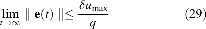
where the positive constant
Proof. Let
We will show

By using equations (27) and (28),
Inaccuracy in flow modeling
Although the spatial basis function well captures the spatial variability of actual flows in a specific region, the function still includes deterministic errors induced by the variability out of the region. In this section, we address the robustness of the proposed adaptive learning algorithm.
To show that the proposed algorithm is robust to disturbance in the flows, we prove the boundedness of CLLE when the actual flow model has unknown disturbances. We assume

The theorem of robustness is proved below.
Theorem 4. Under the same setting of Theorem 1 and
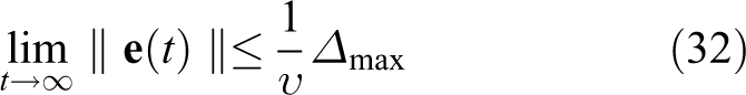
where the positive constant
Proof. Let

We plug the updating rules represented by equations (12) and (13) into equation (33). Then
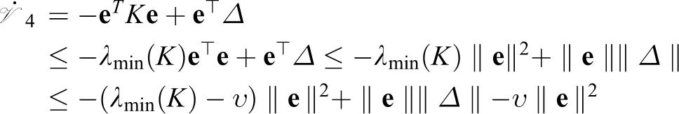
When
Simulations
This section describes simulation results for the anomaly detection algorithms in the section of anomaly detection.
For the presentation of 2D ocean flow,
Figure 1 shows trajectories of a marine robot when the direction of the marine robot in the horizontal plane is controlled by heading angle command

(a) A trajectory under true flow is shown, and (b) the identification error for a simulated trajectory using flow identification is shown. The error is measured by the root-mean-square error between true and simulated trajectories. The identification error converges to 20 s and approaches close to 0 after 100 s.
The flow estimate
Parameters for simulations.

Figure 2 shows simulation results of through-water speed and anomaly detection. In Figure 2(a), two green lines represent the upper and lower bound of normal through-water speed, respectively. When actual through-water speed is reduced to 0.5 m/s after 200 s due to abnormal motion, the learning algorithm keeps tracking actual through-water speed until 300 s.

(a) True through-water speed and (b) flag.
The anomaly detection algorithm changes the value of flag to indicate the status of the simulated robot. The flag value is 2 within the first 10 s, which indicates that a false alarm may happen due to the inaccuracy of identified flow in the initial transient period. The flag value changes to 0 after 10 s because the flow identification error has decreased significantly, as shown in Figure 3, and the identified through-water speed is within the normal range, as shown in Figure 2(a). The flag value switches from 0 to 1 at 200 s because the identified through-water speed is out of the normal range, while the flow identification error is small in Figure 3.

Identification error of flow parameters converges after 20 sec. After 100 s, the identification error converges close to zero. (a) The identification error for the parameters modeling the X-axis component of the flow is shown, and (b) the identification error for the parameters modeling the Y-axis component of the flow is shown.
Experiments and results
The verification of anomaly detection algorithms on marine robots operating in the ocean typically requires significant effort and resource. In addition, generating faults on operational marine robots will induce risk of vehicle loss. Therefore, there is a need for an indoor testbed so that experiments can be carried under controlled conditions with reduced cost and risk. For this purpose, we develop the GT-MAB and the GT-WMR, which are used to collect experimental data on anomaly detection proposed in this article.
Indoor testbed development
The GT-MAB 27 has dynamics that are similar to the dynamics of underwater vehicles. 28 –31 The lighter gas in the GT-MAB induces buoyancy, which plays the same role in restoring force and moment of the GT-MAB as underwater vehicles. The GT-MAB is subjected to significant air dynamic influences, which can be leveraged to emulate flow influences on underwater vehicles.
To generate flow that affects the motion of the GT-MAB, a Dyson fan is used as an artificial wind source. The Dyson fan creates more consistent flows along the direction of blowing wind than rotating fans that produce inconsistent flows. Utilizing the GT-MAB and the Dyson fan, we establish an indoor testbed shown in Figure 4.
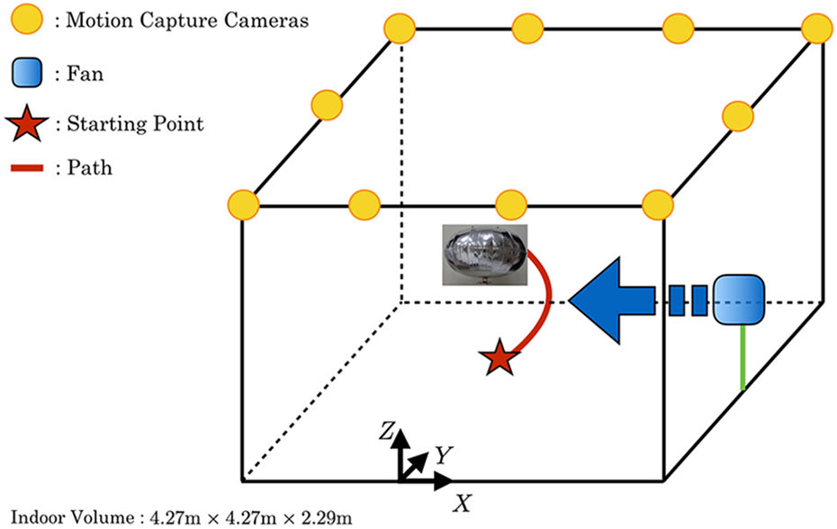
Indoor testbed: The yellow bulbs represent infrared motion capture cameras. The blue square represents the Dyson fan. The star represents the starting point of the GT-MAB. The red line represents the trajectory of the GT-MAB. When the GT-MAB is flying at the starting point, the GT-MAB motion is disturbed by flow generated from the Dyson fan. Then, the motion capture cameras collect the attitudes and trajectory of the GT-MAB. GT-MAB: Georgia Tech Miniature Autonomous Blimp.
Measuring flow generated from the Dyson fan is necessary for algorithm verification. We develop a wind measuring robot (WMR) to measure the wind field of the indoor environment. The GT-WMR collects low wind speed measurements ranged from 0 m/s to 4 m/s in all directions at each location autonomously. As shown in Figure 5, the GT-WMR integrates three wind speed sensors, each with different range and accuracy, on an omnidirectional robot. The GT-WMR autonomously moves along predetermined waypoints, and then, the GT-WMR collects wind measurements at an altitude, where wind sensors are fixed on the omnidirectional robot. These wind measurements enable us to identify the flow field of the Dyson fan.

The GT-WMR contains two main components: an omnidirectional robot called omnibot and three wind sensors. The three wind sensors on a horizontal black frame are connected to the omnibot. The black frame can be moved vertically to measure wind speed at different heights. GT-WMR: Georgia Tech Wind Measuring Robot.
GT-WMR data
To densely collect wind measurements in the indoor testbed, we determine multiple waypoints that can generate the GT-WMR path having a type of lawnmower pattern. Figure 6 shows the waypoints and the GT-WMR’s path, and Figure 7 shows measured wind velocity at each waypoint.

The path (blue) and waypoints (red) of the GT-WMR. GT-WMR: Georgia Tech Wind Measuring Robot.
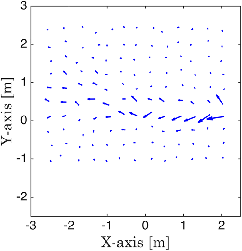
Measured flow velocity at each waypoint.
When the GT-WMR controlled by a waypoint controller accurately reaches one waypoint shown in Figure 6, the GT-WMR stays at the waypoint and changes its orientation with 30° increment starting from 0° to 360°. The wind speed sensors will collect measurements for each of the orientations. The direction where the wind speed is the maximum is chosen as the direction of the wind. Then, the GT-WMR moves to the next waypoint and repeats the measurement process. The measured wind field is plotted in Figure 7. The largest measurement of wind speed is acquired near the wind source. In addition, the width of the area with strong wind is around 0.2 m. This value is similar to the diameter of the Dyson fan, which is 0.254 m. These measurements are consistent with the Dyson fan.
GT-MAB data
We can measure the through-air speed of the GT-MAB, where there is no wind, as 0.0185 m/s. When the Dyson Fan is on, we use the adaptive learning algorithm to identify airflow along the GT-MAB trajectory using the adaptive learning algorithm. Comparing the wind speed measurements with the GR-WMR data will validate the learning algorithm.
For the adaptive learning algorithm, we design four spatial basis functions composed of center ci and width
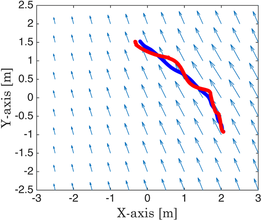
When GT-MAB is operating in normal conditions, the adaptive learning algorithm is applied to identify the flow field. Figure 8 shows measured and identified trajectories of the GT-MAB. At the individual starting point represented by one black square, we select one waypoint along the Y-axis for the forward or backward motion of the GT-MAB. The blue arrows, which represent wind identified by the adaptive learning algorithm, move away from the wind source. The direction of an identified flow corresponds to the wind direction generated from the wind source. Figures 9 and 10 show measured and identified trajectories of the GT-MAB from different starting positions. The magnitude of the blue arrows at the place closing to the wind source is larger than at other places; this tendency corresponds to the fact that strong wind is generated at positions close to the wind source.
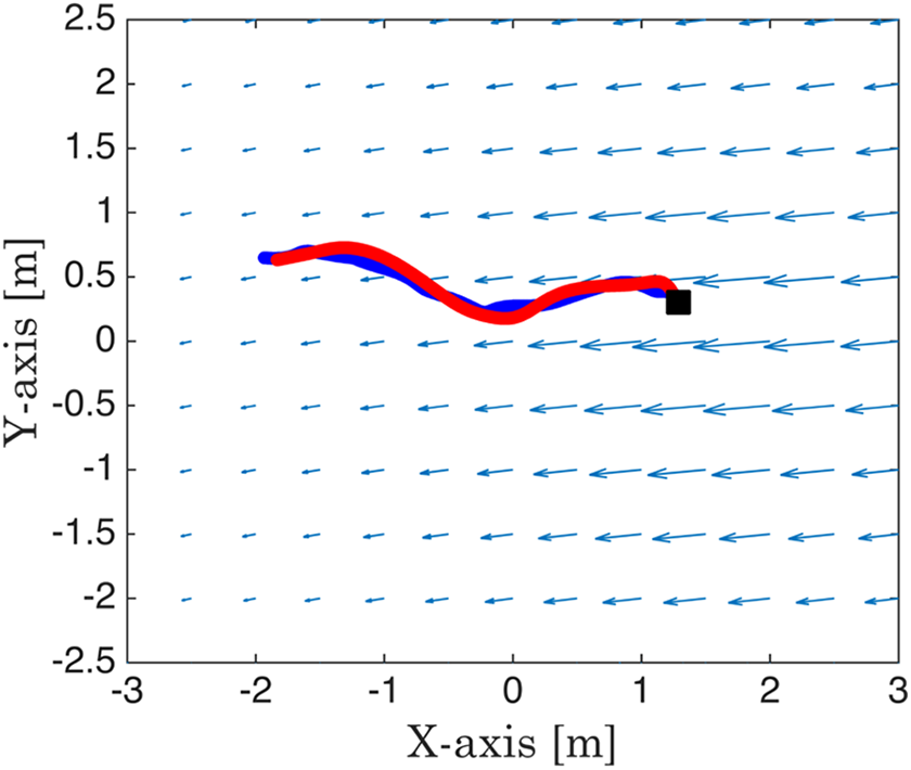
Estimated (blue) and identified (red) trajectories starting at no. 3 (black).
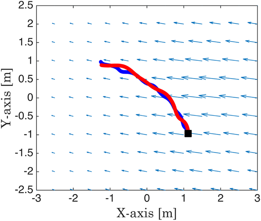
Estimated (blue) and identified (red) trajectories starting at no. 12 (black).

Estimated (blue) and identified (red) trajectories starting at no. 15 (black).
Verifying the adaptive learning algorithm is significantly difficult by simply comparing Figures 8 to 10 with Figure 7. Although wind velocities are identified in the entire space of the testbed, as shown in Figures 8 to 10, the accuracy of the wind velocities is not consistent. Because using constant heading angle command and constant spatial basis functions does not satisfy persistent excitation condition in equation (15), flow parameters for the identified flow may be inaccurately identified. But, nevertheless, this identification is necessary for anomaly detection.
Anomaly detection
The flow estimate
To generate the anomaly, we intentionally disabled a thruster on the GT-MAB to generate a fault and applied the anomaly detection algorithms. The flow parameters are identified by the learning algorithm at the same time. The fault occurs at time

(a, b) Identified through-air speed along the GT-MAB trajectories. GT-MAB: Georgia Tech Miniature Autonomous Blimp.

CLLE along the X-axis (black), and CLLE along the Y-axis (red). CLLE: controlled Lagrangian localization error.
Estimated (blue) and identified (red) trajectories with the identified flow (blue arrow).
Conclusion
The main contribution of this article is two algorithms that detect anomaly of marine robots without sensors monitoring vehicle components: adaptive learning and anomaly detection algorithms. Only using trajectory information, the proposed strategy detects abnormal vehicle motion under unknown ocean flow. It has the potential for mitigating abnormal vehicle motion with path-planning and controller design of marine robots. The experimental results of the GT-MAB and GT-WMR in an indoor testbed verify the proposed strategy. Future work will extend the proposed algorithms to the 3D space for reflecting upwelling flow dynamics. Furthermore, we will incorporate the estimated trajectory from acoustic localization into the proposed algorithms.
Review of adaptive control
We review theorems and lemmas from the theory of adaptive control 24 that are needed for the proofs.
Let

Theorem 5. A necessary and sufficient condition for the uniformly asymptotically stability of the equilibrium of
Definition 1.
32,33
A vector signal u is persistently exciting if there exist positive constants
Lemma 1. Assume that there exist constants
Lemma 2. If
Lemma 3. Consider system
Lemma 4.
34,35
If g is a real function of real variable t, defined and uniformly continuous for
Footnotes
Declaration of conflicting interests
The author(s) declared no potential conflicts of interest with respect to the research, authorship, and/or publication of this article.
Funding
The author(s) disclosed receipt of the following financial support for the research, authorship, and/or publication of this article: This work was supported by ONR grants N00014-19-1-2556, N00014-19-1-2266 and N00014-16-1-2667; NSF grants OCE-1559475, CNS-1828678, and S&AS-1849228; NRL grants N00173-17-1-G001 and N00173-19-P-1412; and NOAA grant NA16NOS0120028.