Kinematic Dexterity Maximization of an Omnidirectional Wheeled Mobile Robot: A Comparison of Metaheuristic and SQP Algorithms

Abstract

Mobile robots with omnidirectional wheels are expected to perform a wide variety of movements in a narrow space. However, kinematic mobility and dexterity have not been clearly identified as an objective to be considered when designing omnidirectional redundant robots. In light of this fact, this article proposes to maximize the dexterity of the mobile robot by properly locating the omnidirectional wheels. In addition, four hybrid differential evolution (DE) algorithm based on the synergetic integration of different kinds of mutation and crossover are presented. A comparison of metaheuristic and gradient-based algorithms for kinematic dexterity maximization is also presented.

1. Introduction

An omnidirectional mobile robot is, in principle, able to move in any arbitrary direction, thus they have been used in several applications, including military [1], human detection [2] and exploration [3] applications. However, most of the time the wheel arrangement of the robot is symmetric, in order to equally distribute the load to each wheel [4]. Kinematic isotropy of a mobile robot [5] is a desired property to get “ease of motion”. One of the key parameters to maximize the isotropy of a mobile robot is the location of the wheels on the body of the robot [6].

Dexterity can be defined as the ability of the robot to move and apply forces and torques in arbitrary directions with equal ease [7]. Poor dexterity of a mobile robot implies that small changes in the linear velocity of the wheels result in large changes in the linear and angular velocity of the robot. High dexterity of the robot means that small changes in the linear velocity of the wheels result in small changes in the linear and angular velocity of the robot.

It is well known that robots designed with optimization methods perform better than robots designed using engineering judgment [3], as they explore all the design space. Therefore, in this paper the optimum wheel placement for the omnidirectional wheeled mobile robot with three omnidirectional wheels is stated as an optimization problem, where the performance index to be optimized is robot dexterity.

Typically, the algorithm selected to solve an optimization problem depends on the problem at hand. There are two main approaches to be considered in the selection of the algorithm and they depend on how the search direction is computed: gradient-based algorithms and heuristic-based algorithms (HBA). Gradient-based algorithms, such as sequential quadratic programming (SQP), are highly dependent on the initial conditions. Convergence to local solutions near the initial condition is the main drawback when SQP is used to solve optimization problems. However, when the initial conditions are in the neighbourhood of a global optimum, most of the time it converges to a better solution when compared to metaheuristic algorithms [8]. Nevertheless, the neighbourhood of the global optimum is not known in real word optimization problems. On the other hand, metaheuristic algorithms (HBA) have been widely used to solve real world optimization problems. Differential evolution (DE) [9] is a metaheuristic algorithm which can be used to solve continuous, discontinuous, linear, nonlinear, dynamic and static optimization problems, that has proven to be useful when designing robots when kinematic singularities should be avoided [10].

DE performs mutations based on the distribution of the solutions in the current population such that the search direction depends on the location and selection of individuals. There are several DE variants, but the most popular is called “DE/rand/1/bin” where just one difference (of two randomly chosen individuals added to another solution) is calculated. Besides the selection of the population size and maximum generation number, an important factor when using DE is the selection of the variant. In those DE variants the mutation and crossover operator is changed and the performance of the DE variants depends on the problem at hand as it is establish in [11].

In this paper the mutation and crossover operator are sinergically combined to improve the characteristics of the DE variant and it is compared with a set of eight DE variants and the performance of the SQP algorithm. This study identifies which algorithm is more suitable to solve the optimization problem at hand.

In order to test the performance of the optimally designed omnidirectional robot, a set of experiments has been performed.

The main motivations of this work are 1) the maximization of the dexterity of the mobile robot by properly locating the omnidirectional wheels, 2) the proposal of four hybrid DE variants that enhance the DE algorithm, 3) the performance evaluation of the chosen algorithms and 4) the analysis of the global and local solution for the trajectory tracking problem.

The remaining material is organized as follows. In Section 2 the kinematics and dynamics of the mobile robot is presented. The optimization problem formulation is stated in Section 3. The optimization algorithm and the proposed hybrid DE variants are described in Section 3. The results and discussion regarding the performance of the algorithms, the optimal design and the simulation results are given in Section 4. Finally, in Section 5 the conclusion is presented.

2. Kinematics and closed-loop dynamics of the mobile robot

The omnidirectional mobile robot is shown in Figure 1 where δ_i and L_i ∀ i=1, 2, 3, are the i –th angle and the i –th distance of the robot wheel. The kinematic transformation between the linear velocity of the wheel v = [v₁, v₂, v₃]^T and the linear and angular velocity of the mobile V_L=[V_x, V_y, w]^T is stated in (1).

Figure 1.

Omnidirectional mobile robot.

$V_L=Av$

(1)

where A ∈ R^3×3 is the Jacobian matrix.

$A=\left[\begin{array}{ccc}-\sin ({\partial }_1)& \cos ({\partial }_1)& L_1\\ -\sin ({\partial }_2)& -\cos ({\partial }_2)& L_2\\ \cos ({\partial }_3)& \sin ({\partial }_3)& L_3\end{array}\right]$

(2)

Considering the mass centre of the omnidirectional mobile robot to be on the origin of the coordinate system x_m-y_m (robot centre), the closed-loop equation for the omnidirectional mobile robot is stated in (1). ${}^{w}V={\left[\begin{array}{ccc}\dot{x_w}& \dot{y_w}& \dot{{\phi }_w}\end{array}\right]}^T\mathrm{,}{}^w\dot{V}$ is the Cartesian and angular velocity and acceleration of the mobile robot with respect to inertial coordinates, τ ∈ R³ is the torque vector of the robot wheels and $e=\hspace{0.17em}{\left[\bar{x}-x_w,\hspace{0.17em}\bar{y}-y_w,\overline{\hspace{0.17em}\phi }-{\phi }_w\right]}^T\in R^3\mathrm{,}\dot{e}=\hspace{0.17em}{\left[\stackrel{.}{\stackrel{̄}{x}}-{\dot{x}}_w,\hspace{0.17em}\stackrel{.}{\hspace{0.17em}\stackrel{̄}{y}}-{\dot{y}}_w,\hspace{0.17em}\stackrel{.}{\stackrel{̄}{\phi }}-{\dot{\phi }}_w\right]}^T\in R^3\in R^3$ are the position and velocity error vectors. The inertia moment and the mass of the mobile robot, the radius and the inertia moment of the wheel are R^3×3 and k_d = diag(k_d1, k_d2, k_d3) ∈ R^3×3 are the proportional and derivative matrix gains.

$\hspace{0.17em}{\bar{M}}_m^w{R}^T{}^w\dot{V}+\left(\bar{M}{\bar{C}}^T+{\stackrel{\sim }{H}}_m^w{R}^T\right){}^{w}V=\bar{B}\tau$

(3)

where:

$\begin{array}{c}\bar{M}=\stackrel{\sim }{M}+\bar{B}\bar{J}{\bar{B}}^T\\ \stackrel{\sim }{M}=diag\left(m,\hspace{0.17em}m,\hspace{0.17em}{I}_z\right)\\ \bar{B}=A^T{\bar{R}}^{-1}\\ {}_m^{w}R=\left[\begin{array}{ccc}\text{cos}(\phi )& -\text{sin}(\phi )& 0\\ \text{sin}(\phi )& \text{cos}(\phi )& 0\\ 0& 0& 1\end{array}\right]\\ \bar{C}=\dot{\phi }\left[\begin{array}{ccc}-\text{sin}(\phi )& -\text{cos}(\phi )& 0\\ \text{cos}(\phi )& -\text{sin}(\phi )& 0\\ 0& 0& 0\end{array}\right]\\ \stackrel{\sim }{H}=\left[\begin{array}{ccc}0& -\dot{\phi }\mathrm{m}& 0\\ \mathrm{m}\dot{\phi }& 0& 0\\ 0& 0& 0\end{array}\right]\\ \breve{Q}={\left(A\hspace{0.17em}{}_m^{w}R\right)}^{-1}\\ u=k_{p}e+k_d\dot{e}\\ \tau ={\breve{Q}}^{T}u\end{array}$

3. Optimization problem statement

Let p= [δ₁, δ₂, δ₃, L₁, L₂, L₃]^T ∈ R⁶ be the design parameters of the wheel locations of a mobile robot. The optimization problem consists of finding the optimal design parameter vector p* ∈ R⁶ such that a small change in the linear velocity of the wheel v or in the Jacobian matrix A results in a small change in the linear and the angular velocity of the mobile V_L, i.e., finding the vector p* such that the mobile robot presents high dexterity.

The condition number of A measures how much the solution of Equation (1) can change in proportion to small changes in the matrix A or in the vector v. A low condition number means that the matrix A is well-conditioned, while high condition number means that matrix A is ill-conditioned. Hence, in this paper the condition number is minimized to improve the dexterity of the mobile robot.

In (3) it is observed that the matrix A can influence the control of the dynamics of the mobile robot. Hence, the robot wheel position improves the robot dexterity for performing a task in the Cartesian space.

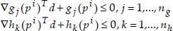
The optimization problem formulation (4 – 5) is to find the optimal design parameter vector p* ∈ R⁶ which minimizes the condition number of the Jacobian (3), subject to the limits in the design parameter vector (4), i.e.,

$\underset{p*}{\min }J=\underset{p*}{\min }{\Vert A|}_F|{A^{-1}\Vert }_F$

(4)

subject to:

$p_{\min }\le p\le p_{\max }$

(5)

The term ‖*‖_F is the Frobenius norm of *. The performance index J = ‖A‖_F‖A⁻¹‖_F can be stated as in (5). It is observed that the problem in (4 – 5) is a nonseparable optimization problem.

$J=\sqrt{\frac{B}{C}}\sqrt{L_1^2+L_2^2+L_3^2+3}$

(6)

$\begin{array}{l}\text{where}B=(4L_1^2+4\cos ({\delta }_1+{\delta }_2)L_1{L}_2+4\sin ({\delta }_1-{\delta }_3)L_1{L}_3+4L_2^2+\\ 4\sin ({\delta }_2+{\delta }_3)L_2{L}_3+4L_3^2-\cos (2{\delta }_1+2{\delta }_2)+\cos (2{\delta }_1-2{\delta }_3)+\\ \cos (2{\delta }_2+2{\delta }_3)+3)\text{and}C=L_1^2\cos (2{\delta }_2+2{\delta }_3)+L_2^2\cos (2{\delta }_1-2{\delta }_3)-\\ L_3^2\cos (2{\delta }_1+2{\delta }_3)+L_1^2+L_2^2+L_3^2+2L_1{L}_3\sin ({\delta }_1+2{\delta }_2+{\delta }_3)+\\ 2L{}^{1}L{}_2\cos ({\delta }_1+{\delta }_2)+2L{}^{2}L{}_3\sin ({\delta }_2+{\delta }_3)+2L{}^{1}L{}_2\cos ({\delta }_1-{\delta }_2-2{\delta }_3)+\\ 2L{}^{2}L{}_3\sin (2{\delta }_1+{\delta }_2-{\delta }_3)+2L{}^{1}L{}_3\cos ({\delta }_1-{\delta }_3).\end{array}$

4. Optimization algorithms

The optimization problem (4 – 5) is solved by using a Sequential Quadratic Programming (SQP) algorithm [11], eight variants of the differential evolution (DE) algorithm [12], [13] and four DE hybrid variants.

4.1 SQP algorithm

SQP algorithm represents the state of the art in nonlinear programming techniques. The SQP algorithm allows to closely mimic Newton's method for constrained optimization just as it is done for unconstrained optimization. At each major iteration, an approximation is made of the Hessian of the Lagrangian function using a quasi-Newton updating method. This is then used to generate a QP subproblem whose solution is used to form a search direction for a line search procedure.

The main idea is the formulation of a quadratic programming (QP) subproblem based on a quadratic approximation of the Lagrangian function (7) where J(p) is the performance function, g_i(p) and h_i(p) are the i-th inequality and equality constraints.

$L(p,\lambda )=J(p)+{\displaystyle \sum _{j=1}^{n_g}{\lambda }_j\cdot g_j(p)+{\displaystyle \sum _{k=1}^{n_h}{\lambda }_k\cdot h_k(p)}}$

(7)

Therefore, the QP subproblem (8 – 9) is obtained by linearizing the nonlinear constraints, where the matrix H_i=∞▽²L is a positive definite approximation of the Hessian matrix of the Lagrangian function (7). H_i is updated by the Broyden-Fletcher-Goldfarb-Shanno (BFGS) method. Hence, if the search direction d_i solves the subproblem given in (8 – 9) and d_i = 0, then the parameter vector p is an optimal solution of the original problem. Otherwise, we set pⁱ⁺¹ = pⁱ + α_id_i and with this new vector the process is repeated again. The step length parameter α_i is determined by an appropriate line search procedure so that a sufficient decrease in the performance index is obtained.

$\underset{p\in n_p}{\min }J\hspace{0.17em}\frac{1}{2}{d}^T{H}_{i}d+\nabla J{(p^i)}^{T}d$

(8)

subject to:

$\begin{array}{l}\nabla g_j{\left(p^i\right)}^{T}d+g_j(p^i)\le 0,\hspace{0.17em}j=1,\dots ,n_g\\ \nabla h_k{\left(p^i\right)}^{T}d+h_k(p^i)\le 0,\hspace{0.17em}k=1,\dots ,n_h\end{array}$

(9)

4.2 Differential evolution variants

This section describes eight different variants of the differential evolution (DE) algorithm and then provides the details of the proposed hybrid DE variant for solving unconstrained optimization problems.

The DE algorithm is composed by four stages (see Figure 2): initialization, mutation, crossover and selection [12]. The main differences among the DE variants are in the mutation and crossover states (row 6 in Figure 2). The general convention used to name the DE variant is DE/x/y/z. DE means Differential Evolution, x represents the vector to be perturbed, y is the number of difference vectors considered for perturbation of x, and z stands for the type of crossover being used (exponential or binomial). The most common DE variants are DE/rand/1/bin, DE/rand/1/exp, DE/best/1/bin, DE/best/1/exp, DE/current-to-rand/1, DE/current-to-best/1, DE/current-to-rand/1/bin and DE/rand/2/dir.

Figure 2.

DE algorithm.

In the initialization stage, the initial population design vector x ⁱ j,G = 0 is randomly generated for all population, where G = 0 indicates the initial generation which the vector belongs, i ∈ [1,…,NP] is a population index, j ∈ [1,…,D] is the design parameter index. This stage is shown in (10), where rand_j(0,1) ∈ [0,1) is a uniformly distributed random number generator and b_j,U, b_j,L indicate the upper and lower limit for the j-th design parameter. For each initial design vector, its objective function is computed.

$\begin{array}{l}For\hspace{0.17em}i\hspace{0.17em}=\hspace{0.17em}0\hspace{0.17em}to\hspace{0.17em}NP\hspace{0.17em}Do\\ \hspace{0.17em}\hspace{0.17em}For\hspace{0.17em}j\hspace{0.17em}=\hspace{0.17em}1\text{\hspace{0.17em}to\hspace{0.17em}}D\hspace{0.17em}Do\\ \hspace{0.17em}{x}_{j,G\hspace{0.17em}=\hspace{0.17em}0}^i\hspace{0.17em}=\hspace{0.17em}ran{d}_j(0,1)(b_{j,U}-b_{j,L})+b_{j,L}\\ \hspace{0.17em}\hspace{0.17em}End\hspace{0.17em}For\\ \text{\hspace{0.17em}\hspace{0.17em}Evaluate\hspace{0.17em}}J({\stackrel{\to i}{x}}_{G\hspace{0.17em}=\hspace{0.17em}0})\\ End\hspace{0.17em}For\end{array}$

(10)

Once the initial population vector is initialized, the mutation stage creates a mutant vector $\stackrel{\to i}{v_G}$ by the mutation and recombination of the individuals of the population. In the crossover stage, trial vector $\stackrel{\to i}{u_G}$ is generated when the target vector $x_{j,G}^i$ is crossed with the mutant vector $\stackrel{\to i}{v_G}$ . The mutation and the crossover stages depend on the DE variant. The mutation and crossover variants are summarized in Figure 3.

Figure 3.

DE variants.

The scale factor F ∈ (0,1) and K ∈ (0,1) in the mutation process, is a positive real number that controls the influence of the selected individuals in order to generate the mutant vector. The indexes r₁, r₂ and r₃ are randomly chosen from the range [1, NP] and the index best represents the individual with the best objective function. Those indexes cannot have the same value.

The crossover probability CR ∈ [0,1] controls the influence of the parent vector in the generation of the offspring (higher values mean less influence of the parent vector, hence higher influence of the mutant vector). It is observed in Figure 3 that the crossover stage does not apply to the current-to-rand/1, current-to-best/1 and rand/2/dir.

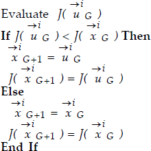
Finally, the last stage involves a selection process between the trial vector $\stackrel{\to i}{u_G}$ and the target vector $x_{j,G}^i$ . First the performance function is evaluated with the trial vector and then an elitism procedure is done where the best of them pass to the next generation. In (11), the selection stage is shown.

$\begin{array}{l}\mathrm{Evaluate}\hspace{0.17em}J({\stackrel{\to i}{u}}_G)\\ If\hspace{0.17em}J({\stackrel{\to i}{u}}_G)<J({\stackrel{\to i}{x}}_G)\hspace{0.17em}Then\\ \hspace{0.17em}\hspace{0.17em}{\stackrel{\to i}{x}}_{G+1}={\stackrel{\to i}{u}}_G\\ \hspace{0.17em}\hspace{0.17em}J({\stackrel{\to i}{x}}_{G+1})=J({\stackrel{\to i}{u}}_G)\\ Else\\ \hspace{0.17em}\hspace{0.17em}{\stackrel{\to i}{x}}_{G+1}={\stackrel{\to i}{x}}_G\\ \hspace{0.17em}\hspace{0.17em}J({\stackrel{\to i}{x}}_{G+1})=J({\stackrel{\to i}{x}}_G)\\ End\hspace{0.17em}If\end{array}$

(11)

4.3 Hybrid DE variant

In our proposal we select four DE variants (rand/1/bin, rand/2/dir, best/1/bin and best/1/exp) to make four hybrid DE algorithms. Those algorithms are named as: Rand/1/bin-Best/1/bin, Best/1/bin-Rand/2/dir, Best/1/bin-Best/1/exp and Rand/2/dir-Best/1/exp. The hybrid variant consists of using two DE variants in each run. The next subsubsection describes the code of the mutation and crossover stages in each hybrid variant and it must be included in line 6 of Figure 2.

4.3.1 Rand/1/bin-Best/1/bin

$\begin{array}{l}\text{Select\hspace{0.17em}randomly\hspace{0.17em}{}{r}_1\ne r_2\ne r_3\text{}\hspace{0.17em}}\in {\overrightarrow{x}}_G\\ \mathrm{Find}\hspace{0.17em}{x}_{j,G}^{best}\text{\hspace{0.17em}in\hspace{0.17em}}{\overrightarrow{x}}_G\\ jrand=\text{randint\hspace{0.17em}(}1,D)\\ For\hspace{0.17em}j=1\text{\hspace{0.17em}to\hspace{0.17em}}D\hspace{0.17em}Do\\ \hspace{0.17em}If{\text{\hspace{0.17em}(rand}}_j[0,1)<CR\text{\hspace{0.17em}or\hspace{0.17em}}j=j_{rand}\text{)\hspace{0.17em}}then\\ Ifi<NP/2\hspace{0.17em}then\\ u_{j,G}^i=x_{j,G}^{r_1}+F(x_{j,G}^{r_2}-x_{j,G}^{r_3})\\ Else\\ u_{j,G}^i=x_{j,G}^{best}+F(x_{j,G}^{r_2}-x_{j,G}^{r_3})\\ EndIf\\ \hspace{0.17em}\hspace{0.17em}Else\\ u_{j,G}^i=x_{j,G}^i\\ \hspace{0.17em}\hspace{0.17em}EndIf\\ EndFor\end{array}$

4.3.2 Best/1/bin-Rand/2/dir

$\begin{array}{l}\text{Select\hspace{0.17em}randomly\hspace{0.17em}{}{r}_1\ne r_2\ne r_3\ne r_4\}\in {\overrightarrow{x}}_G\\ \text{Sort\hspace{0.17em}ascendent\hspace{0.17em}}J({\overrightarrow{x}}_G)\to \stackrel{\to Sort}{x_G}\\ \mathrm{Find}\hspace{0.17em}{x}_{j,G}^{best}\text{\hspace{0.17em}in\hspace{0.17em}}{\overrightarrow{x}}_G\\ \text{Sort\hspace{0.17em}{}{r}_1{r}_2{r}_3{r}_4\text{}\hspace{0.17em}and\hspace{0.17em}keep\hspace{0.17em}it\hspace{0.17em}in\hspace{0.17em}}z\\ j_{rand}\hspace{0.17em}=\text{\hspace{0.17em}randin(1,}D)\end{array}$

$\begin{array}{l}For\hspace{0.17em}j=1\mathrm{to}\hspace{0.17em}D\hspace{0.17em}Do\\ \hspace{0.17em}\hspace{0.17em}If\hspace{0.17em}i<NP/2\hspace{0.17em}Then\\ If{\text{\hspace{0.17em}(rand}}_j\text{[0,1)\hspace{0.17em}}<CR\text{\hspace{0.17em}or\hspace{0.17em}}j=j_{rand}\text{)\hspace{0.17em}}Then\\ u_{j,G}^i=x_{j,G}^{best}+F(x_{j,G}^{r_2}-x_{j,G}^{r_3})\\ \hspace{0.17em}\hspace{0.17em}Else\\ u_{j,G}^i=x_{j,G}^i\\ EndIf\\ \hspace{0.17em}\hspace{0.17em}Else\\ u_{j,G}^i=x_{j,G}^{Sort,z_1}+\frac{F}{2}(x_{j,G}^{Sort,z_1}-x_{j,G}^{Sort,z_2}+x_{j,G}^{Sort,z_3}-x_{j,G}^{Sort,z_4})\\ \hspace{0.17em}EndIf\\ EndFor\end{array}$

4.3.3 Best/1/bin-Best/1/exp

$\begin{array}{l}\text{Select\hspace{0.17em}randomly\hspace{0.17em}{}{r}_1\ne r_2\ne r_3\ne r_4\}\in {\overrightarrow{x}}_G\\ \text{Sort\hspace{0.17em}ascendent\hspace{0.17em}}J({\overrightarrow{x}}_G)\to \stackrel{\to Sort}{x_G}\\ \mathrm{Find}\hspace{0.17em}{x}_{j,G}^{best}\text{\hspace{0.17em}in\hspace{0.17em}}{\overrightarrow{x}}_G\\ \text{Sort\hspace{0.17em}{}{r}_1{r}_2{r}_3{r}_4\text{}\hspace{0.17em}and\hspace{0.17em}keep\hspace{0.17em}it\hspace{0.17em}in\hspace{0.17em}}z\\ j_{rand}\hspace{0.17em}=\text{\hspace{0.17em}randin(1,}D)\\ If\hspace{0.17em}i<NP/2\hspace{0.17em}Then\\ \hspace{0.17em}\hspace{0.17em}For\hspace{0.17em}j=1\text{\hspace{0.17em}to\hspace{0.17em}}D\hspace{0.17em}Do\\ If{\text{\hspace{0.17em}(rand}}_j\text{[0,1)\hspace{0.17em}}<CR\text{\hspace{0.17em}or\hspace{0.17em}}j=j_{rand}\text{)\hspace{0.17em}}Then\\ u_{j,G}^i=x_{j,G}^{best}+F(x_{j,G}^{r_2}-x_{j,G}^{r_3})\\ Else\\ u_{j,G}^i=x_{j,G}^i\\ EndIf\\ \hspace{0.17em}\hspace{0.17em}EndFor\\ Else\\ \hspace{0.17em}\hspace{0.17em}j=j_{rand}\\ \hspace{0.17em}Do\\ u_{j,G}^i=x_{j,G}^{best}+F(x_{j,G}^{r_2}-x_{j,G}^{r_3})\\ j=(j+1)\%D\hspace{0.17em}\\ \hspace{0.17em}\hspace{0.17em}While\hspace{0.17em}rand\text{[0,1)}<CR\text{\hspace{0.17em}and\hspace{0.17em}}j!=j_{rand}\end{array}$

$\begin{array}{l}\hspace{0.17em}\hspace{0.17em}Do\\ u_{j,G}^i=x_{j,G}^{best}+F(x_{j,G}^{r_2}-x_{j,G}^{r_3})\\ j=(j+1)\%D\hspace{0.17em}\\ \hspace{0.17em}\hspace{0.17em}While\hspace{0.17em}rand\text{[0,1)}<CR\text{\hspace{0.17em}and\hspace{0.17em}}j!=j_{rand}\\ \hspace{0.17em}\hspace{0.17em}While\hspace{0.17em}j!=j_{rand}\\ u_{j,G}^i=x_{j,G}^i\\ j=(j+1)\%D\text{\hspace{0.17em}:Modulo\hspace{0.17em}operation}\\ EndWhile\\ EndIf\end{array}$

4.3.4 Rand/2/dir-Best/1/exp

$\begin{array}{l}\text{Select\hspace{0.17em}randomly\hspace{0.17em}{}{r}_1\ne r_2\ne r_3\ne r_4\}\in {\overrightarrow{x}}_G\\ \text{Sort\hspace{0.17em}ascendent\hspace{0.17em}}J({\overrightarrow{x}}_G)\to \stackrel{\to Sort}{x_G}\\ \mathrm{Find}\hspace{0.17em}{x}_{j,G}^{best}\text{\hspace{0.17em}in\hspace{0.17em}}{\overrightarrow{x}}_G\\ \text{Sort\hspace{0.17em}{}{r}_1{r}_2{r}_3{r}_4\text{}\hspace{0.17em}and\hspace{0.17em}keep\hspace{0.17em}it\hspace{0.17em}in\hspace{0.17em}}z\\ j_{rand}\hspace{0.17em}=\text{\hspace{0.17em}randin(1,}D)\\ If\hspace{0.17em}i<NP/2\hspace{0.17em}Then\\ \hspace{0.17em}\hspace{0.17em}For\hspace{0.17em}j=1\text{\hspace{0.17em}to\hspace{0.17em}}D\hspace{0.17em}Do\\ \hspace{0.17em}{u}_{j,G}^i=x_{j,G}^{Sort,z_1}+\frac{F}{2}(x_{j,G}^{Sort,z_1}-x_{j,G}^{Sort,z_2}+x_{j,G}^{Sort,z_3}-x_{j,G}^{Sort,z_4})\\ \hspace{0.17em}EndFor\\ Else\\ j=j_{rand}\\ \hspace{0.17em}\hspace{0.17em}Do\\ u_{j,G}^i=x_{j,G}^{best}+F(x_{j,G}^{r_2}-x_{j,G}^{r_3})\\ j=(j+1)\%D\hspace{0.17em}\\ \hspace{0.17em}While\hspace{0.17em}rand\text{[0,1)}<CR\text{\hspace{0.17em}and\hspace{0.17em}}j!=j_{rand}\\ \hspace{0.17em}\hspace{0.17em}While\hspace{0.17em}j!=j_{rand}\\ u_{j,G}^i=x_{j,G}^i\\ j=(j+1)\%D\text{:Modulo\hspace{0.17em}operation}\\ \hspace{0.17em}\hspace{0.17em}EndWhile\\ EndIf\end{array}$

5. Results and discussion

In this work the SQP algorithm and DE variants are programmed in Matlab Release 7.9 on a Windows platform. Computational experiments were performed on a PC with a 1.83GHz Core 2 Duo processor and 2GB of RAM. One hundred independent runs were carried out for the algorithms.

The initial condition for the SQP algorithm is randomly chosen and the stop criterion is when the change in the performance index value in two consecutive iterations is smaller than 1 × 10⁻¹⁰.

Four parameters must be proposed in order to tune the DE variants. In this case, the population size NP consists of 100 individuals. The scaling factor F and the crossover constant CR are proposed as 0.3, 0.6, 0.9. The K value of the current-to-rand/1 current-to-best/1 and current-to-rand/1/bin DE variants is chosen with the same value of the scaling factor F. The stop criterion is applied when the number of generations is fulfilled G_Max = 300 or when the error between the mean objective function and the global optimum is smaller then 1 × 10⁻¹⁰.

5.1 Performance of the algorithms

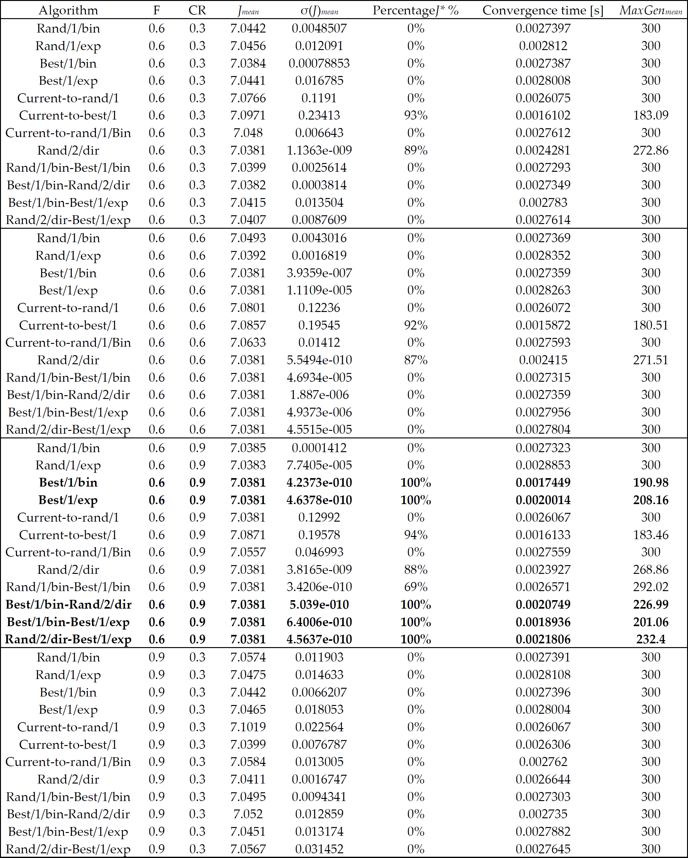
In the Table 1 the performance for 100 independent runs of the SQP algorithm are shown. We realized that the optimization problem (4–5) presents several local solutions. So this optimization problem is multimodal-nonseparable problem.

Table 1.

Performance of the SQP algorithm for 100 independent runs with random initial condition. J_mean: Mean objective function value of individuals of 100 independent runs. Percentage J*: Percentage of runs where the optimal solution is found (at least in one individual of the population). MaxIter_mean: the mean maximum number of iterations.

	Jmean	Percentage J*	Convergence Time [s]	MaxItermean
SQP algorithm	7.6750633252	1%	2.83×10−5	10.3

The best objective function value found is J* = 7.0380710741. Hence we consider it as the global optimal solution to the problem. It is important to comment that the best objective function value is found once (see column 3 in Table 1). Hence, the mean performance of the SQP algorithm is not adequate because the algorithm presents high sensitivity to the initial condition and the optimization problem is a multimodal-nonseparable one. Nevertheless in a real world complex optimization problems, i.e., problems in which the solution is not known, the designer does not know the appropriate number of runs to find the optimal value (the optimal value may not be found). Hence, the importance of using a DE algorithm.

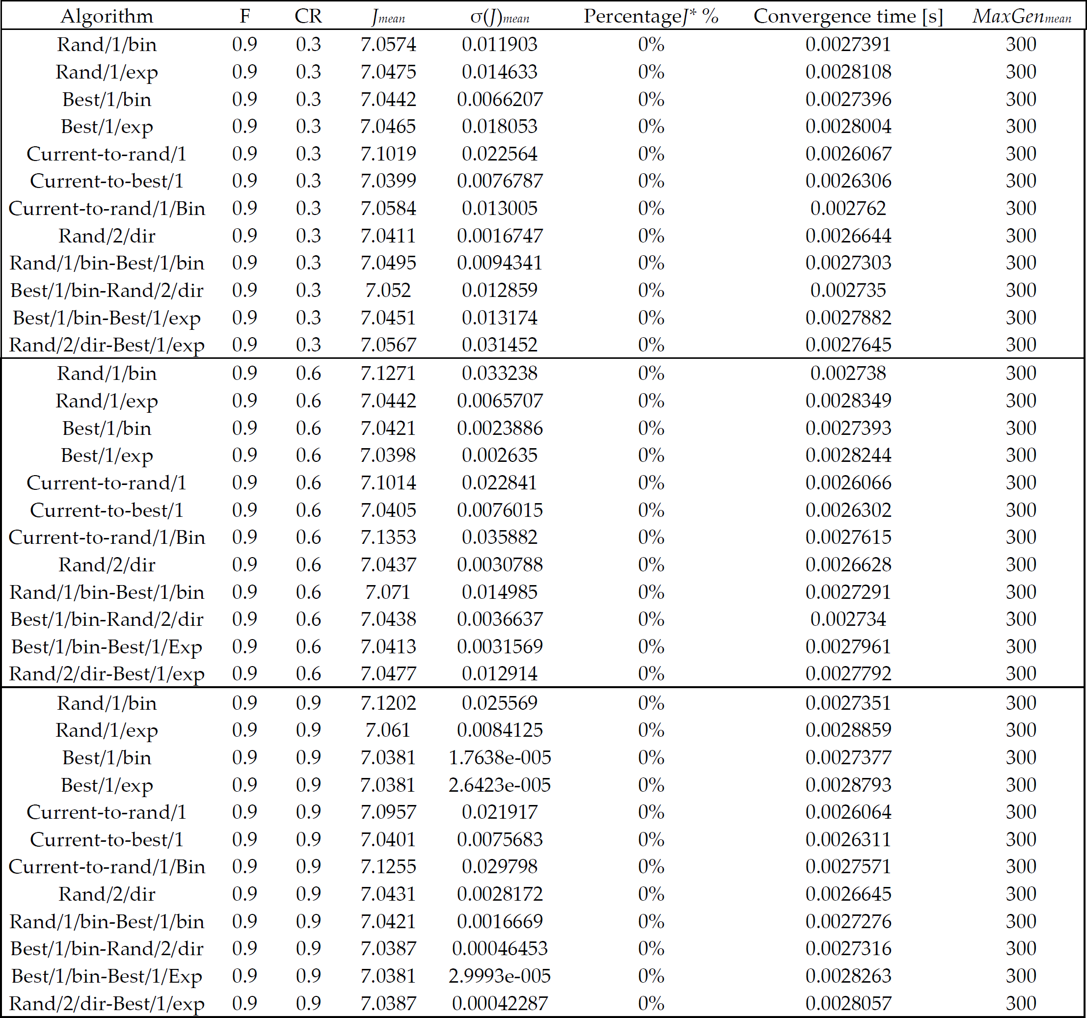
In Table 2-4, the performances of all DE variants for 100 independent runs are presented. Tests with different scaling factor F and crossover constant CR are performed. Tables 2-4 show the mean objective function value, the mean standard deviation, the mean convergence time, the mean iteration for converging the algorithm and the percentage of runs where the optimal solution (considering J* = 7.0380710741 as the optimal solution) is found. The proposed DE variants are mainly analysed taking into account the best convergence to a solution and the standard deviation of the solution. This is because in the real world design problems are stated as optimization problems and the designer requires the “best” design. In that manner, the DE variants which find the best algorithm function with smaller standard deviation will be the “best” algorithm for the particular design problem. A smaller standard deviation guarantees the individuals (solutions) in the last generation are similar, and that those solutions could reach a “global” solution (a global solution may be not guaranteed because the global solution of the nonlinear optimization problem is not known) or a local solution. In the next results, the algorithms whose value of J_mean ≤ 7.0381 are considered are analysed.

Table 2.

Performance of the DE variants. J_mean: Mean objective function value of individuals of 100 independent runs. σ(J_mean): Mean standard deviation (J* – J) of individuals of 100 independent runs. Percentage J*: Percentage of runs where the optimal solution is found. MaxGen_mean: mean maximum generation number of the 100 independent runs.

Algorithm	F	CR	Jmean	σ(J) mean	Percentage J* %	Convergence time [s]	MaxGenmean
Rand/1/bin	0.3	0.3	7.039	0.0011995	0%	0.002741	300
Rand/1/exp	0.3	0.3	7.0439	0.011472	0%	0.0028132	300
Best/1/bin	0.3	0.3	7.0381	8.3224e-006	61%	0.0023223	254.05
Best/1/exp	0.3	0.3	7.0437	0.035027	0%	0.0028045	300
Current-to-rand/1	0.3	0.3	7.8378	0.55255	0%	0.0026072	300
Current-to-best/1	0.3	0.3	7.2885	0.90102	0%	0.0026395	300
Current-to-rand/1/Bin	0.3	0.3	7.0639	0.033516	0%	0.0027617	300
Rand/2/dir	0.3	0.3	7.0702	6.3141e-015	0%	0.0026834	300
Rand/1/bin-Best/1/bin	0.3	0.3	7.0381	0.00015578	0%	0.0027335	300
Best/1/bin-Rand/2/dir	0.3	0.3	7.0381	6.4756e-007	100%	0.0020562	224.91
Best/1/bin-Best/1/exp	0.3	0.3	7.0411	0.025314	4%	0.0027761	299.31
Rand/2/dir-Best/1/exp	0.3	0.3	7.0414	0.026808	34%	0.0027032	293.62
Rand/1/bin	0.3	0.6	7.0383	0.00011191	0%	0.0027393	300
Rand/1/exp	0.3	0.6	7.0381	0.00014856	0%	0.0028363	300
Best/1/bin	0.3	0.6	7.0381	2.1073e-008	99%	0.00083261	91.09
Best/1/exp	0.3	0.6	7.0381	5.2432e-007	100%	0.0017788	188.43
Current-to-rand/1	0.3	0.6	7.8785	0.56759	0%	0.0026076	300
Current-to-best/1	0.3	0.6	7.3097	0.99102	0%	0.0026411	300
Current-to-rand/1/Bin	0.3	0.6	7.0685	0.083518	0%	0.0027592	300
Rand/2/dir	0.3	0.6	7.0643	4.2612e-012	1%	0.002661	298.16
Rand/1/bin-Best/1/bin	0.3	0.6	7.0381	6.9387e-010	100%	0.0015032	164.85
Best/1/bin-Rand/2/dir	0.3	0.6	7.0381	3.9881e-009	100%	0.0011007	120.02
Best/1/bin-Best/1/exp	0.3	0.6	7.0381	6.0731e-006	100%	0.0014183	151.82
Rand/2/dir-Best/1/exp	0.3	0.6	7.0381	6.415e-007	100%	0.0014707	158.1
Rand/1/bin	0.3	0.9	7.0381	3.3208e-010	62%	0.0026356	287.96
Rand/1/exp	0.3	0.9	7.0381	2.5203e-009	35%	0.0028525	295.79
Best/1/bin	0.3	0.9	7.0712	6.6496e-011	15%	0.0017867	265.58
Best/1/exp	0.3	0.9	7.0412	1.7554e-009	67%	0.0013771	152.06
Current-to-rand/1	0.3	0.9	7.8323	0.56999	0%	0.0026076	300
Current-to-best/1	0.3	0.9	7.3051	1.0811	0%	0.0026384	300
Current-to-rand/1/Bin	0.3	0.9	7.2664	0.35754	0%	0.0027559	300
Rand/2/dir	0.3	0.9	7.0766	7.555e-015	0%	0.0026852	300
Rand/1/bin-Best/1/bin	0.3	0.9	7.0381	4.1787e-009	97%	0.00096895	105.98
Best/1/bin-Rand/2/dir	0.3	0.9	7.0387	5.2537e-009	95%	0.00084849	93.86
Best/1/bin-Best/1/exp	0.3	0.9	7.0461	4.7766e-010	36%	0.0017768	218.04
Rand/2/dir-Best/1/exp	0.3	0.9	7.0381	2.4652e-009	98%	0.00087622	92.98

Table 3.

Performance of the DE variants.

Algorithm	F	CR	Jmean	σ(J) mean	Percentage J*%	Convergence time [s]	MaxGenmean
Rand/1/bin	0.6	0.3	7.0442	0.0048507	0%	0.0027397	300
Rand/1/exp	0.6	0.3	7.0456	0.012091	0%	0.002812	300
Best/1/bin	0.6	0.3	7.0384	0.00078853	0%	0.0027387	300
Best/1/exp	0.6	0.3	7.0441	0.016785	0%	0.0028008	300
Current-to-rand/1	0.6	0.3	7.0766	0.1191	0%	0.0026075	300
Current-to-best/1	0.6	0.3	7.0971	0.23413	93%	0.0016102	183.09
Current-to-rand/1/Bin	0.6	0.3	7.048	0.006643	0%	0.0027612	300
Rand/2/dir	0.6	0.3	7.0381	1.1363e-009	89%	0.0024281	272.86
Rand/1/bin-Best/1/bin	0.6	0.3	7.0399	0.0025614	0%	0.0027293	300
Best/1/bin-Rand/2/dir	0.6	0.3	7.0382	0.0003814	0%	0.0027349	300
Best/1/bin-Best/1/exp	0.6	0.3	7.0415	0.013504	0%	0.002783	300
Rand/2/dir-Best/1/exp	0.6	0.3	7.0407	0.0087609	0%	0.0027614	300
Rand/1/bin	0.6	0.6	7.0493	0.0043016	0%	0.0027369	300
Rand/1/exp	0.6	0.6	7.0392	0.0016819	0%	0.0028352	300
Best/1/bin	0.6	0.6	7.0381	3.9359e-007	0%	0.0027359	300
Best/1/exp	0.6	0.6	7.0381	1.1109e-005	0%	0.0028263	300
Current-to-rand/1	0.6	0.6	7.0801	0.12236	0%	0.0026072	300
Current-to-best/1	0.6	0.6	7.0857	0.19545	92%	0.0015872	180.51
Current-to-rand/1/Bin	0.6	0.6	7.0633	0.01412	0%	0.0027593	300
Rand/2/dir	0.6	0.6	7.0381	5.5494e-010	87%	0.002415	271.51
Rand/1/bin-Best/1/bin	0.6	0.6	7.0381	4.6934e-005	0%	0.0027315	300
Best/1/bin-Rand/2/dir	0.6	0.6	7.0381	1.887e-006	0%	0.0027359	300
Best/1/bin-Best/1/exp	0.6	0.6	7.0381	4.9373e-006	0%	0.0027956	300
Rand/2/dir-Best/1/exp	0.6	0.6	7.0381	4.5515e-005	0%	0.0027804	300
Rand/1/bin	0.6	0.9	7.0385	0.0001412	0%	0.0027323	300
Rand/1/exp	0.6	0.9	7.0383	7.7405e-005	0%	0.0028853	300
Best/1/bin	0.6	0.9	7.0381	4.2373e-010	100%	0.0017449	190.98
Best/1/exp	0.6	0.9	7.0381	4.6378e-010	100%	0.0020014	208.16
Current-to-rand/1	0.6	0.9	7.0381	0.12992	0%	0.0026067	300
Current-to-best/1	0.6	0.9	7.0871	0.19578	94%	0.0016133	183.46
Current-to-rand/1/Bin	0.6	0.9	7.0557	0.046993	0%	0.0027559	300
Rand/2/dir	0.6	0.9	7.0381	3.8165e-009	88%	0.0023927	268.86
Rand/1/bin-Best/1/bin	0.6	0.9	7.0381	3.4206e-010	69%	0.0026571	292.02
Best/1/bin-Rand/2/dir	0.6	0.9	7.0381	5.039e-010	100%	0.0020749	226.99
Best/1/bin-Best/1/exp	0.6	0.9	7.0381	6.4006e-010	100%	0.0018936	201.06
Rand/2/dir-Best/1/exp	0.6	0.9	7.0381	4.5637e-010	100%	0.0021806	232.4
Rand/1/bin	0.9	0.3	7.0574	0.011903	0%	0.0027391	300
Rand/1/exp	0.9	0.3	7.0475	0.014633	0%	0.0028108	300
Best/1/bin	0.9	0.3	7.0442	0.0066207	0%	0.0027396	300
Best/1/exp	0.9	0.3	7.0465	0.018053	0%	0.0028004	300
Current-to-rand/1	0.9	0.3	7.1019	0.022564	0%	0.0026067	300
Current-to-best/1	0.9	0.3	7.0399	0.0076787	0%	0.0026306	300
Current-to-rand/1/Bin	0.9	0.3	7.0584	0.013005	0%	0.002762	300
Rand/2/dir	0.9	0.3	7.0411	0.0016747	0%	0.0026644	300
Rand/1/bin-Best/1/bin	0.9	0.3	7.0495	0.0094341	0%	0.0027303	300
Best/1/bin-Rand/2/dir	0.9	0.3	7.052	0.012859	0%	0.002735	300
Best/1/bin-Best/1/exp	0.9	0.3	7.0451	0.013174	0%	0.0027882	300
Rand/2/dir-Best/1/exp	0.9	0.3	7.0567	0.031452	0%	0.0027645	300

Table 4.

Performance of the DE variants.

Algorithm	F	CR	Jmean	σ(J) mean	Percentage J* %	Convergence time [s]	MaxGenmean
Rand/1/bin	0.9	0.3	7.0574	0.011903	0%	0.0027391	300
Rand/1/exp	0.9	0.3	7.0475	0.014633	0%	0.0028108	300
Best/1/bin	0.9	0.3	7.0442	0.0066207	0%	0.0027396	300
Best/1/exp	0.9	0.3	7.0465	0.018053	0%	0.0028004	300
Current-to-rand/1	0.9	0.3	7.1019	0.022564	0%	0.0026067	300
Current-to-best/1	0.9	0.3	7.0399	0.0076787	0%	0.0026306	300
Current-to-rand/1/Bin	0.9	0.3	7.0584	0.013005	0%	0.002762	300
Rand/2/dir	0.9	0.3	7.0411	0.0016747	0%	0.0026644	300
Rand/1/bin-Best/1/bin	0.9	0.3	7.0495	0.0094341	0%	0.0027303	300
Best/1/bin-Rand/2/dir	0.9	0.3	7.052	0.012859	0%	0.002735	300
Best/1/bin-Best/1/exp	0.9	0.3	7.0451	0.013174	0%	0.0027882	300
Rand/2/dir-Best/1/exp	0.9	0.3	7.0567	0.031452	0%	0.0027645	300
Rand/1/bin	0.9	0.6	7.1271	0.033238	0%	0.002738	300
Rand/1/exp	0.9	0.6	7.0442	0.0065707	0%	0.0028349	300
Best/1/bin	0.9	0.6	7.0421	0.0023886	0%	0.0027393	300
Best/1/exp	0.9	0.6	7.0398	0.002635	0%	0.0028244	300
Current-to-rand/1	0.9	0.6	7.1014	0.022841	0%	0.0026066	300
Current-to-best/1	0.9	0.6	7.0405	0.0076015	0%	0.0026302	300
Current-to-rand/1/Bin	0.9	0.6	7.1353	0.035882	0%	0.0027615	300
Rand/2/dir	0.9	0.6	7.0437	0.0030788	0%	0.0026628	300
Rand/1/bin-Best/1/bin	0.9	0.6	7.071	0.014985	0%	0.0027291	300
Best/1/bin-Rand/2/dir	0.9	0.6	7.0438	0.0036637	0%	0.002734	300
Best/1/bin-Best/1/Exp	0.9	0.6	7.0413	0.0031569	0%	0.0027961	300
Rand/2/dir-Best/1/exp	0.9	0.6	7.0477	0.012914	0%	0.0027792	300
Rand/1/bin	0.9	0.9	7.1202	0.025569	0%	0.0027351	300
Rand/1/exp	0.9	0.9	7.061	0.0084125	0%	0.0028859	300
Best/1/bin	0.9	0.9	7.0381	1.7638e-005	0%	0.0027377	300
Best/1/exp	0.9	0.9	7.0381	2.6423e-005	0%	0.0028793	300
Current-to-rand/1	0.9	0.9	7.0957	0.021917	0%	0.0026064	300
Current-to-best/1	0.9	0.9	7.0401	0.0075683	0%	0.0026311	300
Current-to-rand/1/Bin	0.9	0.9	7.1255	0.029798	0%	0.0027571	300
Rand/2/dir	0.9	0.9	7.0431	0.0028172	0%	0.0026645	300
Rand/1/bin-Best/1/bin	0.9	0.9	7.0421	0.0016669	0%	0.0027276	300
Best/1/bin-Rand/2/dir	0.9	0.9	7.0387	0.00046453	0%	0.0027316	300
Best/1/bin-Best/1/Exp	0.9	0.9	7.0381	2.9993e-005	0%	0.0028263	300
Rand/2/dir-Best/1/exp	0.9	0.9	7.0387	0.00042287	0%	0.0028057	300

The results in Table 2-4 show that the best results with F = 0.3 and CR = 0.3 are provided by “Best/1/bin-Rand/2dir”. It presents a convergence to the optimal solution of 100% in all runs, i.e., all runs found the optimal solution, at least once in the population. In addition, it has the smaller mean of maximum generation number (MaxGen_mean) and the convergence time is small. “Rand/2/dir” find local solution due to standard deviation indicates that all individuals of the populations converge to the local solution J_mean = 7.0702. The worst solution is provided by “Current-to-rand/1”.

The best results with F = 0.3 and CR = 0.6 are provided by “Best/1/exp”, “Rand/1/bin-Best/1/bin”, “Best/1/bin-Rand/2/dir”, “Best/1/bin-Best/1/exp” and “Rand/2/dir-Best/1/exp”. It presents a convergence to the optimal solution of 100% in all runs. Those results do not require the maximum generation number to converge to a solution and they provide less convergence time. The standard deviation indicates that “Rand/2/dir” converge to a local solution (J_mean = 7.0643). The worst solution is provided by “Current-to-rand/1”.

The best result with F = 0.3 and CR = 0.9 are provided by “Rand/2/dir-Best/1/exp”. It represents a convergence to the optimal solution of 98% in all runs. The “Best/1/Bin”, “Best/1/Exp” and “Rand/2/Dir” provides local solution (see the standard deviation) in the runs, but the “Best/1/Bin” and the “Best/1/Exp” can reach the optimal solution in some runs. The worst solution is provided by “Current-to-rand/1”.

The best results with F = 0.6 and CR = 0.3 and with F = 0.6 and CR = 0.6 are provided by “Rand/2/dir”. It presents a convergence to the optimal solution of 89% in all runs. It is important to note that the “Current-to-best/1” provides the worst solution in J_mean, nevertheless 92 – 93% of the time it found the optimal solution at least once in the population. Its standard deviation is long and it indicates that the algorithm provides a long diversity in the solution, hence it is not useful in real world problems.

The best results with F = 0.6 and CR = 0.9 are provided by “Best/1/bin”, “Best/1/exp”, “Best/1/bin-Rand/2/dir”, “Best/1/bin-Best/1/exp” and “Rand/2/dir-Best/1/exp”. It presents a convergence to the optimal solution of 100% in all runs. The “Rand/1/Exp” converges to a local solution (see the standard deviation). The worse solution is provided by “Current-to-Best/1”.

The best results with F = 0.9 and CR = 0.3 and with F = 0.9 and CR = 0.6 do not present good solutions. The results with F = 0.9 and CR = 0.9 do not find the optimal value, only “Best/1/Bin”, “Best/1/Exp” and “Best/1/Bin-Best/1/Exp” obtained a closed value to the optimal one.

The results in Table 2–4 show a high sensitivity in the selection of the scaling factor F and the crossover constant CR to get the optimum solution. The empirical results indicate that with F = 0.3 and CR = 0.6 and F = 0.6 and CR = 0.9 the optimal value can be reached in all runs with “Best/1/Exp”, “Best/1/Bin-Rand/2/Dir”, “Best/1/Bin-Best/1/Exp” and “Rand/2/Dir-Best/1/Exp”. A scaling factor of F = 0.9 does not provide good results because it broadens the spectrum of vector differential, such that the optimum solution is not reached in the chosen maximum generation GenMax. In general, the hybrid differential evolution variants provides better results than the DE variants.

The variant “rand/1/bin” is the most useful variant in several real world optimization problems [10],[11]. Nevertheless, the empirical results indicate that this algorithm can only find the global solution at 62% when the scale factor and the crossover probability are chosen as F = 0.3 and CR = 0.9. Moreover the result of the standard deviation shows that the “rand/1/bin” presents a slow convergence to a solution. So, the convergence of the “rand/1/bin” to a solution depends on the selected population number and the maximum number and the maximum generation number.

The main highlights of the results are summarized below:

The optimization problem (4–5) presents several local solutions and it is considered as multimodal-nonseparable problem.

The results of the comparison of the DE variants show that the hybrid differential evolution variant are most competitive that the DE variant because they combine the advantage of using two different variants in the runs.

Regarding the real word optimization problems, the algorithms that find the best results are “Best/1/Exp”, “Best/1/Bin-Rand/2/Dir”, “Best/1/Bin-Best/1/Exp” and “Rand/2/Dir-Best/1/Exp”, because they provide in all runs the convergence to the optimal solution. In addition, they present a rapid convergence towards a solution without becoming stuck in a local minimum.

The rand/1/bin could converge to suboptimal solutions if the generation number is not appropriately selected.

The SQP algorithm requires less computational time that the DE variants. Nevertheless, the main drawbacks of using SQP algorithm are the high sensitivity to the initial condition when a nonlinear optimization problem is solved. Besides, the optimization problem must be continuously differentiable twice in order to compute both the gradient vector and the Hessian matrix. In addition, a constraint handling mechanism must be included when constrained optimization problems are solved.

The DE variants are easier to implement than the SQP algorithm. In addition, a special constraint handling mechanism for the upper and lower constraint in the design variables is not required because it is included in the original DE algorithm [14].

In real world complex optimization problems the use of a hybrid DE variant to solve them provides more competitive results than a DE variant.

5.2 Optimal design

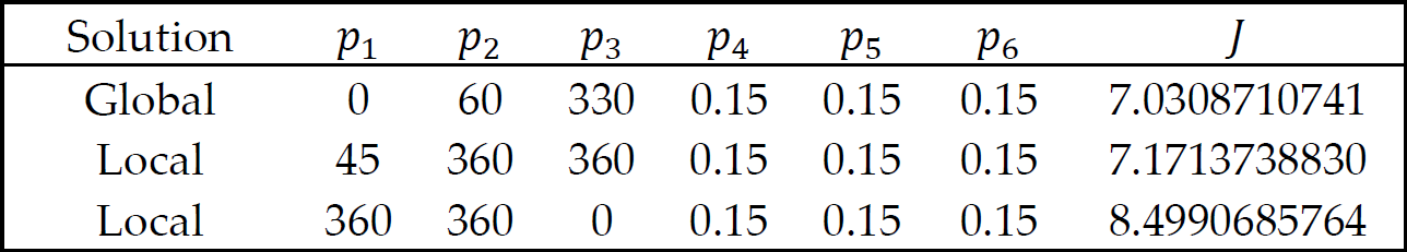
In Table 5 the performance index of the global and two local solutions (location of the robot wheel) using the SQP algorithm are shown. The optimal design of the location of the robot wheel for those solutions is presented in Figure 4. As stated before, several local solutions exist in the optimization problem (4–5). Nevertheless, in some local solutions the angles δ₁, δ₂, δ₃, are different in spite of having the same performance index. Analysing the results, we realize that there are several angle combinations that result in the same local and global performance function. Two particular local solutions (J = 8.4990685764 and J = 7.1713738830) and the global solution (J* = 7.0380710741) are analysed. The main relation among the designs with the particular performance function of 8.4990685764 is that the angle α_i ∀ _i = 1,…3 (see Figure 4c) must have whatever combination of the following angles: $\pi ,\hspace{0.17em}\frac{\pi }{2}$ and $\frac{\pi }{2}$ radians. The designs with the performance function of 7.1713738830 requires that the angles α _i ∀ _i = 1,…3 (see Figure 4b) must have whatever combination of the following angles: $\frac{3\pi }{4},\hspace{0.17em}\frac{\pi }{2}$ and $\frac{3\pi }{4}$ radians. Finally, the designs with the global performance function of 7.0380710741 requires that the angles α_i ∀ _i = 1,…3 (see Figure 4a) must have $\frac{2\pi }{3}$ radians.

Table 5.

Global and two particular local solutions found by the SQP algorithm. Units in degrees and metres.

Solution	p 1	p 2	p 3	p 4	p 5	p 6	J
Global	0	60	330	0.15			7.0308710741
Local	45	360	360	0.15			7.1713738830
Local	360	360	0	0.15			8.4990685764

Figure 4.

Global and local solutions for the optimal location of the omnidirectional robot wheels.

In Figure 5 the computer aided design (CAD) and the real photo of the optimum design for the omnidirectional wheeled mobile robot are shown.

Figure 5.

CAD and real photo of the design with optimum dexterity of an omnidirectional wheeled mobile robot.

5.3 Simulation results

The simulation results consist of controlling the dynamics of the omnidirectional mobile robot to follow a desired trajectory considering the three different wheel configurations in Table 5. A proportional derivative (PD) control is used for the simulation results.

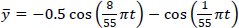
A Runge Kutta method is used to solve the nonlinear differential Equation (11). The initial conditions are chosen as ^wV(t₀ = 0) = 0 ∈ R³, x(t₀ = 0) = 0, y(t₀ = 0) = 0, φ(t₀ = 0) = 0 and the integration step of 1ms with final time t_f = 120s. The desired trajectories are shown in (12)-(14). The gains of the PD controller and the parameters of the mobile robot are selected as

^wV(t₀ = 0) = 0 ∈ R³, x(t₀ = 0) = 0, y(t₀ = 0) = 0, φ(t₀ = 0) = 0 and the integration step of 1ms with final time t_f = 120s. The desired trajectories are shown in (12)-(14). The gains of the PD controller and the parameters of the mobile robot are selected as k_p1 = k_p2 = 7, k_p3 = 3, k_d1 = k_d2 = 10, k_d3 = 0.5 and I_z = 0.0127Kgm², m = 11.8316Kg, J_i = 5.82E – 4Kgm², r_i = 0.0625m ∀ _i = 1,2,3, respectively.

$\hspace{0.17em}\bar{x}=0.5\sin \left(\frac{8}{55}\pi t\right)+\sin \left(\frac{1}{55}\pi t\right)$

(12)

$\bar{y}=-0.5\cos \left(\frac{8}{55}\pi t\right)-\cos \left(\frac{1}{55}\pi t\right)$

(13)

$\bar{\phi }=\pi \sin \left(\frac{1}{55}\pi t\right)$

(14)

The trajectory tracking of the mobile robot for the three different wheel location (see Table 5) are shown in Fig. 6. The behaviour of the mobile robot looks similar. For that reason, in Table 6, the sum of the L₂ -norm of the position error signals and the sum of the L₂-norm of the input signals are presented. It is observed that the mobile robot with the optimum wheel location (J^*) can achieve a smaller position error. Hence, good dexterity is an important factor in providing the mobile robot with the ability to move in arbitrary directions with more precision. Considering Eq. (1), if A is well-conditioned, large or small variations in v imply large or small variations in V_L.

Table 6.

Sum of the L₂-norm of the position error signals and the sum of the L₂-norm of the input signals.

	|e1|2+|e2|2 [m]	|e3|2 [rad]
J*	0.9141	5.4483e-007
J1	0.9142	6.3975e-004
J2	0.9143	7.2705e-004

Figure 6.

Trajectory tracking with different wheel location.

6. Conclusion

In this paper the formulation of the optimal dexterity of an omnidirectional mobile robot is proposed as an optimization problem. The empirical comparison of the SQP algorithm, eight different DE variants and four proposed hybrid DE variants for this particular optimization problem is presented. The obtained results show that the mutation and crossover stages are important factors in the search for the solution in multimodal-nonseparable problems. Then, the proposed hybrid DE variants provide a better mechanism to find the solution. The SQP algorithm presents a high sensitivity to the initial condition. So the performance of the DE variants is more consistent in the search for the optimal solution and they are not sensitive to the initial set of solutions. However, the computational time is higher than those required by the SQP algorithm.

From the engineering design point of view, a hybrid heuristic approach must be considered first and then a gradient approach, in order to finely search in the complete space and hence find the best design.

The condition number is a useful measure to achieve high robot dexterity. High dexterity indicates that linear and angular velocity of the mobile robot increase/decrease with a similar rate as the linear velocity of the wheel.

The control performance of the mobile robot not only depends on the appropriate selection of the controller gains, it depends on the mechanical design aspects such as the robot dexterity.