A trajectory planning method for the redundant manipulator based on configuration plane

Abstract

This study focuses on the method of trajectory planning of spatial obstacle avoidance for redundant manipulators based on configuration plane method. Firstly, according to the summary of the work configuration for redundant manipulator, kinematics analysis method based on configuration plane is proposed, which helps to establish a basic kinematics model of configuration plane. Secondly, the analysis of velocity is conducted and velocity iterative formula is derived. Then, the process of the trajectory planning for redundant manipulator based on the velocity distribution of configuration plane is given, during which some key procedures such as the determination of work configuration, achieving spatial obstacle avoidance, and analysis of velocity distribution are deduced. Finally, the simulation of spatial circle trajectory planning for the 7-degree-of-freedom redundant manipulator is done. The experimental results show that the proposed trajectory planning method for redundant manipulator can satisfy the requirements of complex spatial obstacle avoidance and increase the controllability of the trajectory between spatial interpolation points of the manipulator’s end effector.

Introduction

Kinematic redundancies in robotic motion planning and control bring several benefits such as improved manipulability, controllability, collision avoidance, flexibility, dexterity, larger workspace, and singularity avoidance. ¹ Manipulators with kinematic redundancies possess more degrees of freedom (DOFs) than those strictly necessary to perform a given task. ²

To begin with, several traditional methods have been employed in trajectory planning. For example, a planning method of trajectory motion for serial-link manipulators with higher degree polynomials application has been proposed by Boryga and Grabos. ³ In the study of Liu et al., ⁴ the strategy has been designed as a combination of the planning with multi-degree splines in Cartesian space and multi-degree B-splines in joint space to generate smooth trajectories. Many research activities have also been implemented to acquire optimum paths and trajectories considering dynamic constraints such as time and velocity with serial manipulators of multiple DOFs, and the corresponding literature is quite sufficient. For instance, Chwa et al. have used the manipulators to intercept the fast-flying object, and the joint velocity constraints and torque constraints are applied to the motion trajectory of the manipulators. ⁵ Saravanan et al. ⁶ have employed the Nonuniform Rational B Spline (NURBS) curve to conduct the trajectory planning of the manipulator to optimize the motion time to satisfy various requirements of motion constraints. Ashwini Shukla et al. have proposed a path planner for serial manipulators with multiple DOFs, working in cluttered workspace, and this method involves formulating the path planning problem as constrained minimization of a function representing the total joint movement over the complete path based on the variational principles. ⁷ Other trajectory optimization methods can be found in the literatures. ^{8 –13} Kinematic redundancy of robots allows simultaneous execution of several tasks with different priorities. Additionally, obstacle avoidance is one of the common subtasks beside the main task, and the ability to avoid obstacles is especially significant in those human interaction tasks. Therefore, several attempts have also been made to consider obstacles in trajectory planning generation process. ¹⁴ In the work of Capisani et al., ¹⁵ an n-joint planar manipulator has been considered, assuming that obstacles located in its workspace can be approximated in a conservative way with circles. In the study of Petrič and Žlajpah, ¹⁶ a novel control method for robots with kinematic redundancy has been proposed based on a new and very simple null-space formulation, which focuses on a smooth as well as continuous transition between different tasks. Zacharia et al. introduce a method for simultaneously planning collision-free motion and scheduling time-optimal route along a set of given task points. ¹⁷ Meanwhile, this method is based on the projection of the workspace and the robot on the B-surface to formulate an objective function for the minimization of the cycle time in visiting multiple task points and takes into account the multiple solutions of the inverse kinematics and the obstacle avoidance.

A great deal of intelligent algorithms have been carried out to resolve those problems of dynamic constraints and obstacle avoidance of redundant manipulators as well. Zha has presented a unified approach to optimal pose trajectory planning for robot manipulators in Cartesian space through a genetic algorithm (GA) enhanced optimization of the pose ruled surface. ¹⁸ Focusing on calculating inverse kinematics and obstacle avoidance for complex unknown environments with multiple obstacles in the working field, a new approach for solving the problem of obstacle avoidance during manipulation tasks performed by redundant manipulators is proposed, and the developed solution is based on a double neural network that uses Q-learning reinforcement technique. ¹⁹ In the work of Chyan and Ponnambalam, ²⁰ four variants of particle swarm optimization (PSO) are proposed to solve the obstacle avoidance control problem of redundant robots. The four variants of PSO are namely PSO-W, PSO-C, qPSO-W, and qPSO-C, where the latter two algorithms are hybrid version of the first two.

The trajectory planning methods introduced in the above part are based on the spline curve to conduct the trajectory planning of the manipulator’s end effector. In addition, the angles of each joint are obtained using inverse kinematics method of the manipulator. There are two kinds of methods for inverse kinematics method of the manipulator including analytical solutions and numerical solutions. However, the effectiveness of analytical solutions is greatly dependent on the topological structure of the redundant manipulator, which lacks generality; although numerical solutions are suitable for the inverse kinematics of various types of manipulators, it is difficult to realize in those occasions which has a high real-time requirement for manipulators. In addition, the motion trajectory of the manipulator’s end effector is generated by the joint motion of the redundant manipulator, which leads to the discreteness of the trajectory of the end effector at the interpolation points. The configuration plane method has the advantages of fast inverse kinematics solution and is independent of the specific working configuration. ²¹

Inspired by the manuscript above, a universal trajectory planning method for the redundant manipulator based on configuration plane within the consideration of collisions is proposed. The main contributions in the article are summarized as follows: Firstly, the trajectory planning method based on configuration plane can not only reduce the calculation burden but also extend the generality for the majority of various redundant manipulators. Secondly, the velocity distribution based on configuration plane technique is able to deal with the incontinuity and uncontrollability of motion trajectory between interpolation points during the motion process of the manipulator.

Therefore, this article proposes a trajectory planning method based on configuration plane. At the same time, the velocity distribution based on configuration plane technique was also proposed to deal with the incontinuity and uncontrollability of motion trajectory between interpolation points during the motion process of the manipulator.

The article is organized as follows. In the second and third sections, the basis of the planning method is detailed. The fourth section is devoted to present the trajectory planning method based on the configuration. In the fifth section, a real case of simulation is carried out to test the effectiveness of the method. The article closes with conclusions and references.

Fundamentals and problem proposing

The common path planning method for redundant manipulator

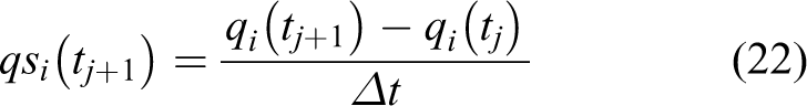
The spatial trajectory of the redundant manipulator’s end effector is composed of a series of key points in the joint space. Assume that the ith (i = 1, 2,…, ns) sequence point is p_i , and ns is defined as the number of these sequence points. In the meanwhile, $\left\{t_1, t_2,\dots ,t_{ns}\right\}$ is the corresponding time series. These key points are able to meet the requirements of the manipulator’s obstacle avoidance or the specified trajectory, such as a straight line, arc, or spline curve.

If the position and orientation matrix of point p_i at time t_i is known, the angles of joints can be obtained using inverse kinematics method of the redundant manipulator. Assume that the number of manipulator’s joint is m, and the angle of the jth (j = 1, 2,…, m) joint at time t_i is ${\theta }_j(t_j)$ . To ensure the manipulator’s motion continuity and stability, linear function with polynomial blends connects the j th joint’s angles at the two adjacent time, as shown in equation (1)

${\theta }_j\left(t\right)=a_{kj}{t}^k+a_{k-1j}{t}^{k-1}+\dots +a_{0j}$

1

where k is the degree of polynomial. $a_{kj},a_{k-1j}, \dots , a_{0j}$ is the coefficients of polynomial and can be defined by the method proposed by Boryga and Grabos.³ The velocity, acceleration, and jerk of joint can be obtained through the differential of joint angle.

The kinematic constraint

As the number of redundant manipulator’s DOF is larger than the spatial DOF, the value of jth joint’s angle at time t_i is not unique. The spatial joint constraints are shown in the following equations

${\theta }_{j\text{min}}\le {\theta }_j\left(t\right)\le {\theta }_{j\text{max}}\left(j=1,\dots , m\right)$

2

$\left|{\dot{\theta }}_j\left(t\right)\right|\le v_{j\text{max}}\left(j=1,\dots ,m\right)$

3

$\left|{\ddot{\theta }}_j\left(t\right)\right|\le {\alpha }_{j\text{max}}\left(j=1,\dots ,m\right)$

4

where ${\dot{\theta }}_j\left(t\right)$ is the velocity of the manipulator’s jth joint, $v_{j\text{max}}$ is the maximum velocity of the manipulator’s jth joints, ${\ddot{\theta }}_j(t)$ is the acceleration of the manipulator’s jth joint, and ${\alpha }_{j\text{max}}$ is the maximum acceleration of the manipulator’s jth joint.

In addition, due to the increase in the value of the second-order acceleration, the tracking error of joint’s position will be increased too. Simultaneously, to increase the service life and decrease the excessive loss of the manipulator, second-order acceleration constraints are proposed,⁵ as shown in equation (5)

$\left|{\stackrel{⃛}{\theta }}_j\left(t\right)\right|\le {\chi }_{j\text{max}}\left(j=1,\dots ,m\right)$

5

where ${\chi }_{j\text{max}}$ is the maximum jerk of the manipulator’s jth joint.

The optimization method kinematic constraint

The multiple solutions of the inverse kinematics provide more choices for trajectory planning of redundant manipulators. So many researchers have conducted extensive studies on optimization methods. The optimized function decides whether these optimized methods are effective or not. The optimized function proposed in the work of Saravanan et al.⁶ can achieve the optimal time and energy during the trajectory planning process, as shown in equation (6)

$f={\xi }_1{\displaystyle \sum _{i=1}^n\left(t_i-t_{i-1}\right)}+{\xi }_2\left(\alpha {\displaystyle \sum _{i=1}^n{\displaystyle \sum _{j=1}^m{\left({\dot{\theta }}_{ij}{\tau }_{ij}\right)}^2\left(t_i-t_{i-1}\right)}}\right)$

6

where ${\xi }_1$ and ${\xi }_2$ are the weighted coefficients of time optimized function and energy optimized function, separately. Setting ${\xi }_1+{\xi }_2=1$ , when ${\xi }_1=1$ , the optimization goal of trajectory planning is the optimal time. α is the elastic coefficient. The value of α can be adjusted to decrease the difference value between energy consumption and time in magnitude. ${\tau }_{ij}$ is the torque of the jth joint at the ith key point.

The method of path planning using optimized function to find the optimal path is numerical method in the population search way, such as PSO method, A* algorithm, and GA.

Problem proposing

1. The trajectory planning methods introduced above are based on the inverse kinematics of redundant manipulators. Therefore, these methods overall depend on the topological structure of the redundant manipulator. In addition, the methods for inverse kinematics with generality and low-scale computation burden are quite important for the practicability of redundant manipulators.

2. The method that the optimized function regarded as the optimized goal to obtain the optimal trajectory in the population search way does not take into account the dynamic effect in local trajectory planning, which can result that the motion in some region is not rational as well as the whole load of a joint is not average. Therefore, when the manipulator runs with full load or full speed, there exist local defects during the whole trajectory planning process.

As shown in Figure 1, in the initial period of motion process, the change values of angular velocity of each manipulator’s joint relative to the whole motion process are relatively large, but they are relatively small in the later period of motion process. The optimal result is obtained using optimized function method, as shown in Figure 2, where the horizontal axis represents the running time and the vertical axis represents the rotation angles of each joint. However, it is not rational in the view of the overall motion process, and the movement is not stable in the initial period of motion process.

Figure 1.

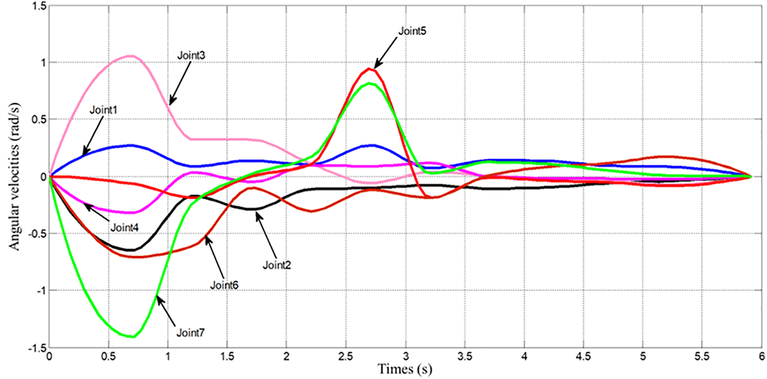
The angular velocity of each joint based on the optimized function.

• 3. As the polynomial blends of joint angle in joint space, the motion between the two key points of the manipulator’s end effector is not controllable, which may generate an unexpected trajectory motion. Figure 2 shows the manipulator in the process of linear motion. The polynomial blends of the manipulator’s each joint at two adjacent time are conducted to ensure the stability of the motion. Since the polynomial blends are based on a few key points of the straight line, the trajectory of the manipulator’s end effector between the key points is irregular and jumping, so it does not satisfy the requirements of strict trajectory in some industrial operations. For example, when a welding robot is welding, the irregular motion of the manipulator’s end effector will not only make the welding uneven but also can injure the manipulator’s end effector.

Figure 2.

The actual trajectory of the manipulator’s end effector in the process of straight-line motion.

The objective of this article is to design a method of trajectory planning that can effectively avoid obstacles for redundant manipulators based on configuration plane method with universality, which can enhance the planning efficiency, reduce the computation burden, and strengthen the controllability and smoothness.

Kinematics analysis method based on configuration plane

Definition of configuration plane

In the topological structures of the typical serial manipulator, however the joints of the manipulator move, a plane composed of central axes of sequentially connecting robotic links is called configuration plane. As shown in Figure 3, the mechanism of the manipulator is usually composed of several configuration planes, the number of which is less than the number of manipulator’s joints. However, for some manipulators including bias swing joints, however the joints of the manipulator move, the central axes of sequentially connecting robotic links are parallel to or included in a plane which is called virtual configuration plane. To limit the number of virtual configuration planes, we define that the virtual configuration plane must include a central axis of a manipulator’s link.

Figure 3.

Basic model of the configuration plane.

Kinematics analysis of the configuration plane

The motion joints of serial manipulator can be classified into three basic types, that is, prismatic joint, revolute joint, and swinging joint. The motion joint with multiple DOFs can be decomposed into a single DOF motion joint. Figure 4 shows the schematic diagram of configuration plane modeling. The first joint of the configuration plane is the revolute joint. In addition, the center of the revolute joint’s rotational axis is the center of the configuration plane which is point O, as shown in Figure 4. The rotational axis of the revolute joint coincides with the Z axis. The other joints are a plurality of swing joints and prismatic joints in the configuration plane. The rotation axis of the swing joint is parallel to the Y axis. Without losing generality, prismatic joints and swinging joints can be in arbitrary position in the configuration plane. The terminal of the configuration plane is the center of the next revolute joint’s rotational axis which is point P, as shown in Figure 4.

Figure 4.

Schematic diagram of velocity iterative calculation among the configuration planes.

The schematic diagram of the configuration plane is shown in Figure 4, the kinematic model of which is shown in the following equation

$CP=\left[\begin{array}{cccc}\text{cos}\theta & -\text{sin}\theta & 0& 0\\ \text{sin}\theta & \text{cos}\theta & 0& 0\\ 0& 0& 1& p_z^{″}\\ 0& 0& 0& 1\end{array}\right]\left[\begin{array}{cccc}\text{cos}\beta & 0& \text{sin}\beta & p_x^{\prime }\\ 0& 1& 0& 0\\ -\text{sin}\beta & 0& \text{cos}\beta & p_z^{\prime }\\ 0& 0& 0& 1\end{array}\right]$

7

In the right of equation (7), there are two homogeneous transformation matrices. In the first matrix on the right-hand side of equation (7), $\theta$ is the rotational angle of the revolute joint in the configuration plane and $p_z^{″}$ is the structural parameter of the revolute joint. The second matrix on the right-hand side of equation (7) represents the homogeneous matrix of swing and prismatic joints which are sequentially connected in the configuration plane. In the second matrix, $\beta ={\beta }_2+\dots +{\beta }_n$ , where ${\beta }_i\left(i=2\dots n-1,n\right)$ is the ith rotational angle of the swing joint. If the ith joint is a prismatic joint, then ${\beta }_i$ is zero. $p_x^{\prime }$ and $p_z^{\prime }$ are the obtained parameters based on the multiplication of transformation matrix for swing and prismatic joints, expressions of which are shown in equations (8) and (9)

$p_x^{\prime }=h_n\text{cos}\left({\beta }_2+\dots +{\beta }_n\right)+\dots +h_2\text{cos}\left({\beta }_2\right)$

8

$p_z^{\prime }=h_n^{\prime }\text{sin}\left({\beta }_2+\dots +{\beta }_n\right)+\dots +h_2^{\prime }\text{sin}\left({\beta }_2\right)$

9

where $h_i\left(i=2\dots n\right)$ and $h_i^{\prime }\left(i=2\dots n\right)$ are the length of link which connects the ith swing joint. $h_i^{\prime }\left(i=2\dots n\right)$ is the sum of fixed length and movement of prismatic joint.

Figure 4 describes the standard configuration plane. In addition, several special configuration planes are shown in the following part.

If the first joint of the manipulator is not the revolute joint, the parameter $\theta$ of the revolute joint in equation (7) is zero.

The end effector of a manipulator is usually a revolute joint, to guarantee position and orientation requirements, and the parameters of swing and prismatic joints in equation (7) are zero.

The virtual configuration plane is caused by the bias of the central axes of two sequentially connecting swing joints. Therefore, in equation (7), the value of bias is added, as shown in equation (10)

$CP=\left[\begin{array}{cccc}\text{cos}\theta & -\text{sin}\theta & 0& 0\\ \text{sin}\theta & \text{cos}\theta & 0& 0\\ 0& 0& 1& p_z^{″}\\ 0& 0& 0& 1\end{array}\right]\left[\begin{array}{cccc}\text{cos}\beta & 0& \text{sin}\beta & p_x^{\prime }\\ 0& 1& 0& p_y^{\prime }\\ -\text{sin}\beta & 0& \text{cos}\beta & p_z^{\prime }\\ 0& 0& 0& 1\end{array}\right]$

10

On the condition that there are multiple connecting angles of link joint for the manipulator, the link joint can be regarded as a special revolute joint, the joint angle $\theta$ of which is the fixed in equation (7).

Analysis of velocity based on configuration plane

Analysis of velocity within the configuration plane

The expression of joint variables, that is $\theta$ , can be obtained based on equation (1). Then, the velocity of joint variables, that is $\dot{q}$ , can be obtained through the differential of equation (1). Then, the following equation can be obtained

$\dot{p}=J\dot{q}$

11

where $\dot{p}\in R^{6\times 1}$ is the velocity of the terminal of configuration plane which is point p relative to the center of configuration plane which is point O, as shown in Figure 4. J is the one order influence coefficient matrix of the configuration plane, which is Jacobian matrix. If the joint is revolute and swing joints, the expression of Jacobian matrix is shown in equation (12). If the joint is the prismatic joint, the expression of Jacobian matrix is shown in equation (13). $\dot{q}\in R^{n\times 1}$ is the generalized velocity of joint variable, which includes the velocity of swing joint, revolute joint, and prismatic joint

$J=\left[\begin{array}{ccccc}-\text{sin}\theta {\displaystyle \sum _{i=2}^n{h}_i}\text{cos}\left({\displaystyle \sum _{j=2}^i{\beta }_j}\right)& \dots & -\text{cos}\theta {\displaystyle \sum _{i=kk}^n{h}_i}\text{sin}\left({\displaystyle \sum _{j=2}^i{\beta }_j}\right)& \dots & -h_n\text{cos}\theta \text{sin}\left({\displaystyle \sum _{i=2}^n{\beta }_i}\right)\\ \text{cos}\theta {\displaystyle \sum _{i=2}^n{h}_i}\text{cos}\left({\displaystyle \sum _{j=2}^i{\beta }_j}\right)& \dots & -\text{sin}\theta {\displaystyle \sum _{i=kk}^n{h}_i}\text{sin}\left({\displaystyle \sum _{j=2}^i{\beta }_j}\right)& \dots & -h_n\text{sin}\theta \text{sin}\left({\displaystyle \sum _{j=2}^n{\beta }_j}\right)\\ 0& \dots & {\displaystyle \sum _{i=kk}^n{h}_i}\text{cos}\left({\displaystyle \sum _{j=2}^i{\beta }_j}\right)& \dots & h_n\text{sin}\left({\displaystyle \sum _{j=2}^n{\beta }_j}\right)\\ 0& \dots & \text{cos}\theta \text{sin}\left({\displaystyle \sum _{j=2}^{kk-1}{\beta }_j}\right)& \dots & \text{cos}\theta \text{sin}\left({\displaystyle \sum _{j=2}^{n-1}{\beta }_j}\right)\\ 0& \dots & \text{sin}\theta \text{sin}\left({\displaystyle \sum _{j=2}^{kk-1}{\beta }_j}\right)& \dots & \text{sin}\theta \text{sin}\left({\displaystyle \sum _{j=2}^{n-1}{\beta }_j}\right)\\ 1& \dots & \text{cos}\left({\displaystyle \sum _{j=2}^{kk-1}{\beta }_j}\right)& \dots & \text{cos}\left({\displaystyle \sum _{j=2}^{n-1}{\beta }_j}\right)\end{array}\right]$

12

$J=\left[\begin{array}{ccccc}-\text{sin}\theta {\displaystyle \sum _{i=2}^n{h}_i}\text{cos}\left({\displaystyle \sum _{j=2}^i{\beta }_j}\right)& \dots & \text{cos}\theta \text{cos}\left({\displaystyle \sum _{j=2}^{kk}{\beta }_j}\right)& \dots & -h_n\text{cos}\theta \text{sin}\left({\displaystyle \sum _{i=2}^n{\beta }_i}\right)\\ \text{cos}\theta {\displaystyle \sum _{i=2}^n{h}_i}\text{cos}\left({\displaystyle \sum _{j=2}^i{\beta }_j}\right)& \dots & \text{sin}\theta \text{cos}\left({\displaystyle \sum _{j=2}^{kk}{\beta }_j}\right)& \dots & -h_n\text{sin}\theta \text{sin}\left({\displaystyle \sum _{j=2}^n{\beta }_j}\right)\\ 0& \dots & \text{sin}\left({\displaystyle \sum _{j=2}^{kk}{\beta }_j}\right)& \dots & h_n\text{sin}\left({\displaystyle \sum _{j=2}^n{\beta }_j}\right)\\ 0& \dots & 0& \dots & \text{cos}\theta \text{sin}\left({\displaystyle \sum _{j=2}^{n-1}{\beta }_j}\right)\\ 0& \dots & 0& \dots & \text{sin}\theta \text{sin}\left({\displaystyle \sum _{j=2}^{n-1}{\beta }_j}\right)\\ 1& \dots & 0& \dots & \text{cos}\left({\displaystyle \sum _{j=2}^{n-1}{\beta }_j}\right)\end{array}\right]$

13

Analysis of velocity among the configuration planes

According to topological structure of the manipulator, there exists velocity coupling phenomenon among configuration planes. The velocity of configuration plane, that is ${\dot{p}}_i$ , near the robotic base has an influence on which is near the robotic end effector.

As shown in Figure 4, assume that ${\dot{p}}_i$ is the velocity exerted on the ith configuration plane by the former $i-1$ configuration planes. Its component relative to the robotic base coordinate is expressed as $\left\{{\upsilon }_x^i,{\upsilon }_y^i,{\upsilon }_z^i,{\omega }_x^i,{\omega }_y^i,{\omega }_z^i\right\}$ . The component of velocity generated by each joint in the ith configuration plane relative to the configuration plane’s coordinate system is expressed as $\left\{{\upsilon }_{cpx}^i,{\upsilon }_{cpy}^i,{\upsilon }_{cpz}^i,{\omega }_{cpx}^i,{\omega }_{cpy}^i,{\omega }_{cpz}^i\right\}$ . The component of velocity generated by the terminal of the ith configuration plane relative to the robotic base coordinate system is expressed as $\left\{{\upsilon }_x^{i+1},{\upsilon }_y^{i+1},{\upsilon }_z^{i+1},{\omega }_x^{i+1},{\omega }_y^{i+1},{\omega }_z^{i+1}\right\}$ . $r_i^{i+1}$ is the space vector from the center of the ith configuration plane to the terminal of the ith configuration plane.

The component of which relative to the configuration plane’s coordinate system is expressed as $\left\{r_{cpx}^i,r_{cpy}^i,r_{cpz}^i\right\}$ and the component of which relative to the robotic base is expressed as $\left\{r_x^i,r_y^i,r_z^i\right\}$ . Assuming the rotation matrix of the center of the ith configuration plane’s coordinate frame relative to the robotic base coordinate frame is R_i , R_i is $3\times 3$ matrix. The following equation can be obtained.

Then, the component of linear velocity and angular velocity for each configuration plane can be expressed as equations (14) to (16)

$\left[\begin{array}{c}{r}_x^i\\ r_y^i\\ r_z^i\end{array}\right]=R_i\left[\begin{array}{c}{r}_{cpx}^i\\ r_{cpy}^i\\ r_{cpz}^i\end{array}\right]$

14

$\left[\begin{array}{c}{v}_x^{i+1}\\ v_y^{i+1}\\ v_z^{i+1}\end{array}\right]=\left[\begin{array}{c}{r}_x^i{\omega }_x^i\\ r_y^i{\omega }_y^i\\ r_z^i{\omega }_z^i\end{array}\right]+R_i\left[\begin{array}{c}{v}_{cpx}^i\\ v_{cpy}^i\\ v_{cpz}^i\end{array}\right]+\left[\begin{array}{c}{v}_x^i\\ v_y^i\\ v_z^i\end{array}\right]$

15

$\left[\begin{array}{c}{\omega }_x^{i+1}\\ {\omega }_y^{i+1}\\ {\omega }_z^{i+1}\end{array}\right]=R_i\left[\begin{array}{c}{\omega }_{cpx}^i\\ {\omega }_{cpy}^i\\ {\omega }_{cpz}^i\end{array}\right]+\left[\begin{array}{c}{\omega }_x^i\\ {\omega }_y^i\\ {\omega }_z^i\end{array}\right]$

16

The process of trajectory planning

The method of determining working configuration for redundant manipulator

According to the velocity iterative calculation of the configuration plane introduced in the former section, the primary condition to obtain velocity decomposition is that the working configuration of the redundant manipulator at a certain time in workspace is known. As the redundant manipulator has redundant spatial DOFs, its work configuration at a certain position in its workspace is not unique. Thus, it can satisfy the following requirements.

• 1. The position and orientation requirements of spatial trajectory point

To define the work configuration of the redundant manipulator, the solution of the inverse kinematics is obtained. Assume that the position and orientation matrix of spatial trajectory point at time t_j is $TP\left(t_j\right)$ , and the number of configuration planes that make up the redundant manipulator is ncp. According to the expression of configuration plane, that is equation (10), we can get the following equation

$TP\left(t_i\right)=C{P}_1\left(t_i\right)*C{P}_2\left(t_i\right)*\dots *C{P}_{ncp}\left(t_i\right)$

17

The common redundant manipulator is composed of two or three configuration planes. In each configuration plane, two parameters are used to describe the orientation of the configuration plane. The two parameters can be obtained using the analytical method. Then, the joints of redundant DOF can achieve the position and obstacle avoidance requirements at spatial trajectory point. If the redundant manipulator is composed of four configuration planes, the parameters which describe the orientation of certain configuration plane are known. However, a manipulator that has more than eight DOFs composed of more than four configuration planes is not discussed in this article because it belongs to the hyper-redundant manipulator. As shown in Figure 5, some values of joint variables can be obtained using the analytical method to satisfy the orientation requirement. The preliminary work configuration can be obtained using spatial vector projection method based on the previous research by our group. ²¹ Simultaneously, the other unknown joint variables are also obtained. Wei et al. ²² use the weighted space vector method to solve the inverse kinematics of 6R serial robot.

Figure 5.

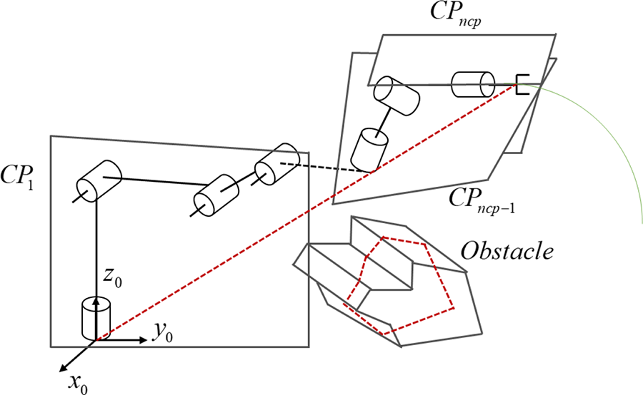
Spatial obstacle avoidance for the redundant manipulator.

• 2. The requirement of spatial obstacle avoidance

To achieve spatial obstacle avoidance, for redundant manipulator, the first step is to detect whether the manipulator interferes with obstacles during its spatial motion period. As the redundant manipulator has been decomposed into configuration planes of finite numbers, the preliminary work configuration of the redundant manipulator is known. Additionally, the spatial expression of the configuration plane is also known, and the expression of spatial obstacle in each of the configuration planes could be obtained using spatial analytical geometry method. Then, the link and obstacles in the configuration plane are calculated separately.

In this article, the description method of space obstacles is based on the configuration plane method. The collision detection of space obstacles based on the configuration plane is carried out after the redundant manipulator completes the trajectory planning of the end effector of the manipulator. The spatial position and expression of the configuration plane that makes up the manipulator have been determined, and the configuration of the configuration plane and the interference detection between obstacles are needed. There are two cases of noninterference between the manipulator and obstacles in the configuration plane: In the first case, the configuration plane where the manipulator is located does not intersect with the obstacle; in the second case, the configuration plane of the manipulator intersects with the obstacle, but the manipulator itself does not interfere with the obstacle. Because the first case is relatively simple, it is not discussed and we focus on the second case.

As shown in Figure 6, obstacles in the three-dimensional space are crosscut into a cross-sectional figure by the two-dimensional plane where the configuration plane is located. This cross-sectional figure may be very irregular and is covered by relatively simple successively connected linear segments. Considering the external size and safe distance of the robot connecting rod, the distance h is extended outward in the obstacle area 1, so that the actual area of the obstacle changes into the state of area 2.

Figure 6.

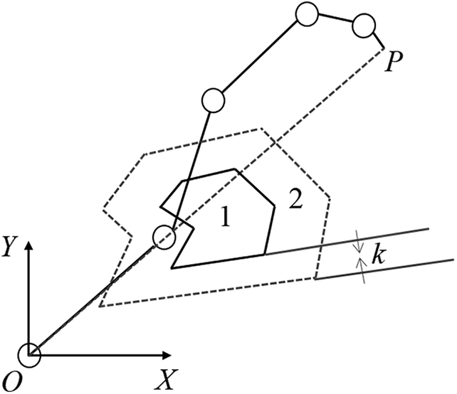
Interference check of the configuration plane and obstacle.

Assume that the safety obstacle avoidance area consists of line segments of m, the line segment can be expressed as

$z_a=\frac{\left(z_i-z_{i-1}\right)\left(x_i-x_{i-1}\right)}{x_i-x_{i-1}}+z_{i-1}$

18

The robot configuration is composed of n line segments, and the line segment of segment j is expressed as

$z_b=\frac{\left(z_j-z_{j-1}\right)\left(x_j-x_{j-1}\right)}{x_j-x_{j-1}}+z_{j-1}$

19

In plane geometry, two lines are either parallel or intersect. Hence, to improve the efficiency of the judgment process, we first compare whether the slopes of the two-line segments expressed by equations (18) and (19) are equal. If they are not equal, we need to solve the intersection point of the line where the two-line segments are. Then it is easy to judge whether the intersection point is between the two-line segments. According to the trajectory planning process of the redundant manipulator, the center and the end of the configuration plane cannot be in the obstacle region, otherwise the redundant manipulator cannot complete the task. Therefore, the joint part of the manipulator interferes with the boundary segment that constitutes the safety obstacle area. In order to improve the overall robot planning calculation efficiency, it is not necessary to judge all robot joints and all line segments that constitute the safety obstacle area, we only need to readjust the interference joint in the configuration plane and judge the boundary line segment between the interference joint and the safety obstacle area near the robot base.

As shown in Figure 6, k is the spatial distance between the link and obstacle which is also called spatial safety distance. According to the trajectory planning process of the redundant manipulator, the center and the end of the configuration plane cannot be in the obstacle region, otherwise the redundant manipulator cannot complete the work. Therefore, the joint part of the robot interferes with the boundary segment that constitutes the safety obstacle area. To improve the whole robot programming calculation efficiency, without the need for total judgment in the area between the lines of the manipulator joints and the lines of safety barrier area, only interference joint on the configuration of the plane should be readjusted and the border lines between interference joints and security obstacle area near the base should be judged.

After the interference detection between spatial obstacle and manipulator, the link in the interfering part needs to be readjusted using spatial vector projection method, as shown in Figure 7. Equation (18) shows the spatial vector projection method

$‖p‖={\displaystyle \sum _{i=0}^n{a}_i{h}_i}$

20

where $‖p‖$ is the norm of vector from the terminal of the configuration plane to its center and a_i is the ratio between link i and vector $\overrightarrow{p}$ . As the projection of vector is directional, a_i has a plus or minus sign. Its expression is shown in equation (19)

$a_i=h_i\text{cos}\left({\theta }_i^{\prime }\right)$

21

where ${\theta }_i^{\prime }$ is the angle between link i and the vector of target points.

Figure 7.

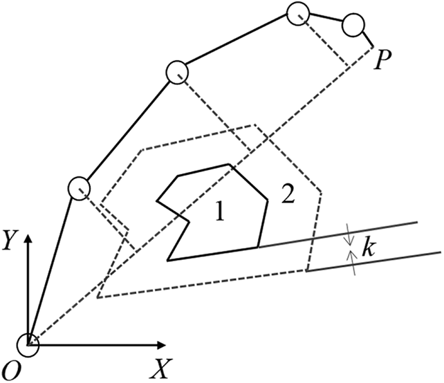
Obstacle avoidance of the manipulator’s joint in the configuration plane.

Velocity distribution among configuration planes

In the former section, the work configuration of the redundant manipulator has been defined according to the position and orientation requirement of spatial trajectory point. However, to ensure that the end effector of the manipulator move continuously during the motion process, the velocity distribution of each joint is conducted in the work configuration of each spatial trajectory point. For the redundant manipulator, as the relationship between the velocity of joint and end effector is nonlinear and highly coupled, the configuration plane method is used to conduct velocity distribution.

The velocity distribution of the redundant manipulator based on the configuration plane is starting from the configuration plane including the end effector of the manipulator. According to the manipulator’s topology, the configuration plane is treated as a unit and the velocity distribution of the configuration plane is conducted from the last configuration plane to the first including the robotic base one by one.

The velocity distribution is based on equations (15) and (16), as $\left\{r_{cpx}^i,r_{cpy}^i,r_{cpz}^i\right\}$ and $R_i^{i+1}$ are known, and the linear and angular velocity distribution is conducted. Assume that the angle of each joint in the previous adjacent spatial trajectory point is $q_i\left(t_j\right)$ , $i=1,2,\dots m$ , t_j is the time node during movement. Additionally, the angle of each joint movement in the current spatial trajectory point is $q_i\left(t_{j+1}\right)$ . The time interval is $\Delta t=t_{j+1}-t_j$ . The average movement speed of each joint between the two trajectory points can be obtained by equation (22)

$q{s}_i\left(t_{j+1}\right)=\frac{q_i\left(t_{j+1}\right)-q_i\left(t_j\right)}{\Delta t}$

22

Based on the velocity obtained by equation (16), the end effector velocity of the manipulator can be obtained using the method introduced in the second section. The velocity solution in the configuration plane and the velocity iteration of the configuration plane. Its component relative to the base coordinate frame is $\left\{\upsilon s_x^{ },\upsilon s_y^{ },\upsilon s_z^{ },\omega s_x^{ },\omega s_y^{ },\omega s_z^{ }\right\}$ . While the target velocity component of the current trajectory point relative to the base coordinate frame is $\left\{{\upsilon }_x^{ }\left(t_{j+1}\right),{\upsilon }_y^{ }\left(t_{j+1}\right),{\upsilon }_z^{ }\left(t_{j+1}\right),{\omega }_x^{ }\left(t_{j+1}\right),{\omega }_y^{ }\left(t_{j+1}\right),{\omega }_z^{ }\left(t_{j+1}\right)\right\}$ , then the error between the two velocities is shown in equation (23)

$\left[\begin{array}{c}\Delta {\upsilon }_x\\ \Delta {\upsilon }_y\\ \Delta {\upsilon }_z\\ \Delta {\omega }_x\\ \Delta {\omega }_y\\ \Delta {\omega }_z\end{array}\right]=\left[\begin{array}{c}{\upsilon }_x\left(t_{j+1}\right)-\upsilon s_x\\ {\upsilon }_y\left(t_{j+1}\right)-\upsilon s_y\\ {\upsilon }_z\left(t_{j+1}\right)-\upsilon s_z\\ {\omega }_x\left(t_{j+1}\right)-\omega s_x\\ {\omega }_y\left(t_{j+1}\right)-\omega s_y\\ {\omega }_z\left(t_{j+1}\right)-\omega s_z\end{array}\right]$

23

According to equations (15) and (16), the velocity of the terminal of the configuration plane relative to the base coordinate frame is composed of two parts. One part is the velocity generated by the current configuration plane, and the other part is the velocity exerted on the center of the current configuration plane by the previous adjacent configuration plane. Hence, the error obtained in equation (23) can be distributed into the joints in each configuration plane. We can assign the motion velocity deviation generated from equation (23) to each joint of the configuration plane.

Assume that the velocity increment of the terminal of the ith configuration plane is ${\left[\begin{array}{cccccc}\Delta {\upsilon }_x^{i+1}& \Delta {\upsilon }_y^{i+1}& \Delta {\upsilon }_z^{i+1}& \Delta {\omega }_x^{i+1}& \Delta {\omega }_y^{i+1}& \Delta {\omega }_z^{i+1}\end{array}\right]}^{\text{T}}$ and the velocity increment of the center of the ith configuration plane (the terminal of $\left(i-1\right)$ th configuration plane) is ${\left[\begin{array}{cccccc}\Delta {\upsilon }_x^i& \Delta {\upsilon }_y^i& \Delta {\upsilon }_z^i& \Delta {\omega }_x^i& \Delta {\omega }_y^i& \Delta {\omega }_z^i\end{array}\right]}^{\text{T}}$ . Then, equations (24) and (25) can be obtained based on equations (15) and (16).

The components of the linear velocity and angular velocity of the configuration plane can be expressed as equations (24) and (25)

$\left[\begin{array}{c}{\upsilon }_x^{i+1}+\Delta {\upsilon }_x^{i+1}\\ {\upsilon }_y^{i+1}+\Delta {\upsilon }_y^{i+1}\\ {\upsilon }_z^{i+1}+\Delta {\upsilon }_z^{i+1}\end{array}\right]=\left[\begin{array}{c}{r}_x^i\left({\omega }_x^i+\Delta {\omega }_x^i\right)\\ r_y^i\left({\omega }_y^i+\Delta {\omega }_y^i\right)\\ r_z^i\left({\omega }_z^i+\Delta {\omega }_z^i\right)\end{array}\right]+R_i\left[\begin{array}{c}{\upsilon }_{cpx}^i\\ {\upsilon }_{cpy}^i\\ {\upsilon }_{cpz}^i\end{array}\right]+\left[\begin{array}{c}{\upsilon }_x^i+\Delta {\upsilon }_x^i\\ {\upsilon }_y^i+\Delta {\upsilon }_y^i\\ {\upsilon }_z^i+\Delta {\upsilon }_z^i\end{array}\right]$

24

$\left[\begin{array}{c}{\omega }_x^{i+1}+\Delta {\omega }_x^{i+1}\\ {\omega }_y^{i+1}+\Delta {\omega }_y^{i+1}\\ {\omega }_z^{i+1}+\Delta {\omega }_z^{i+1}\end{array}\right]=R_i\left[\begin{array}{c}{\omega }_{cpx}^i\\ {\omega }_{cpy}^i\\ {\omega }_{cpz}^i\end{array}\right]+\left[\begin{array}{c}{\omega }_x^i+\Delta {\omega }_x^i\\ {\omega }_y^i+\Delta {\omega }_y^i\\ {\omega }_z^i+\Delta {\omega }_z^i\end{array}\right]$

25

Based on equations (24) and (25), the velocity of the terminal of the ith configuration plane relative to its center coordinate frame is obtained, as shown in equations (26) and (27)

$\left[\begin{array}{c}{\upsilon }_{cpx}^i\\ {\upsilon }_{cpy}^i\\ {\upsilon }_{cpz}^i\end{array}\right]=R_i^{-1}\left(\left[\begin{array}{c}{\upsilon }_x^{i+1}+\Delta {\upsilon }_x^{i+1}\\ {\upsilon }_y^{i+1}+\Delta {\upsilon }_y^{i+1}\\ {\upsilon }_z^{i+1}+\Delta {\upsilon }_z^{i+1}\end{array}\right]-\left[\begin{array}{c}{r}_x^i\left({\omega }_x^i+\Delta {\omega }_x^i\right)\\ r_y^i\left({\omega }_y^i+\Delta {\omega }_y^i\right)\\ r_z^i\left({\omega }_z^i+\Delta {\omega }_z^i\right)\end{array}\right]-\left[\begin{array}{c}{\upsilon }_x^i+\Delta {\upsilon }_x^i\\ {\upsilon }_y^i+\Delta {\upsilon }_y^i\\ {\upsilon }_z^i+\Delta {\upsilon }_z^i\end{array}\right]\right)$

26

$\left[\begin{array}{c}{\omega }_{cpx}^i\\ {\omega }_{cpy}^i\\ {\omega }_{cpz}^i\end{array}\right]=R_i^{-1}\left(\left[\begin{array}{c}{\omega }_x^{i+1}+\Delta {\omega }_x^{i+1}\\ {\omega }_y^{i+1}+\Delta {\omega }_y^{i+1}\\ {\omega }_z^{i+1}+\Delta {\omega }_z^{i+1}\end{array}\right]-\left[\begin{array}{c}{\omega }_x^i+\Delta {\omega }_x^i\\ {\omega }_y^i+\Delta {\omega }_y^i\\ {\omega }_z^i+\Delta {\omega }_z^i\end{array}\right]\right)$

27

According to equation (11), the velocity of each joint can be obtained, as shown in equation (28)

${\left[\begin{array}{cccc}{\dot{\theta }}^i& {\dot{\beta }}_2^i& \dots & {\dot{\beta }}_n^i\end{array}\right]}^{\text{T}}=J_i^{-1}{\left[\begin{array}{cccccc}{\upsilon }_{cpx}^i& {\upsilon }_{cpy}^i& {\upsilon }_{cpz}^i& {\omega }_{cpx}^i& {\omega }_{cpy}^i& {\omega }_{cpz}^i\end{array}\right]}^{\text{T}}$

28

Trajectory planning between interpolation points

The motion path of the manipulator’s end effector is generated by the joint motion of the serial manipulator, so it is highly coupling and nonlinear, which results in the discreteness of the trajectory path of robotic end effector at the interpolation points. The trajectory planning of interpolation points can not only ensure the controllability of the movement of robotic end effector at interpolation points but also avoid collisions between manipulator and obstacles. In addition, most of the existing trajectory planning methods are based on position not velocity of the manipulator. Hence, in this article, the trajectory planning of interpolation points can be generalized based on the velocity distribution of the configuration plane according to the redundancy of the redundant manipulator.

The planning process is shown in Figure 8, and the manipulator’s end effector moves between the two interpolation points S1 and S2. The trajectory between S1 and S2 is a continuous line segment relative to time, which is expressed in equation (29)

$S=f\left(x,y,z,t\right)$

29

Figure 8.

The velocity planning process between interpolation points.

The concrete expression of equation (29) is related to the trajectory during the actual motion, and S1 is the initial point and S2 is the t terminal point.

According to equation (29), the velocity of robotic end effector at point S1 can be obtained. According to the velocity distribution based on the configuration plane introduced in the third section, the velocity of the configuration plane can be obtained too. After running $\Delta t$ time, the manipulator reaches the point of b1. $\Delta t$ is called the compensation cycle here. Due to the nonlinear and high coupling characteristics of the redundant robot manipulator motion, from Figure 8, there is a spatial bias between the manipulator’s end effector and the predetermined trajectory. So, compensation adjustment is necessary. The manipulator’s end effector is moved to point a1 rather than point b1 which is in turn, until completing the movement to point S2.

In the process of the motion planning, the line between point S1 and point b1 is not a straight line but a linear motion, depended on the speed distribution of the configuration plane in a short period of time.

In addition, as the change of the manipulator’s end effector is relatively large by using compensation adjustment introduced above, as shown in Figure 8, the difference value between point b1 and actual motion point a1 is relatively large too. Therefore, based on equation (29), the acceleration of the manipulator’s end effector at interpolation point can be obtained. Additionally, the direction and magnitude of the velocity of the manipulator’s end effector at the initial point of motion can be adjusted according to the obtained acceleration value, as shown in Figure 9. The motion error is greatly reduced by this method.

Figure 9.

The velocity planning improvement between interpolation points.

The trajectory planning method of the interpolation points is based on the inverse kinematics solution which satisfies spatial obstacle avoidance using configuration method and the velocity distribution based on configuration plane method. For general redundant and hype-redundant manipulators, its work configuration consists of two to four configuration planes. Additionally, the trajectory between the interpolation points is to eliminate the uncontrollability of the motion between the interpolation points and reduce the error of trajectory motion. Therefore, the compensation period is short. In a word, the motion planning method introduced in this section not only greatly reduces computation time and motion error during the process of the planning movement but also increases the controllability of the movement.

Simulation analysis of examples

In this section, we take a 7-DOF redundant manipulator as an example for simulation analysis and introduce the trajectory planning method for the redundant manipulator.

The model of degrees of freedom redundant manipulator

The joint parameters of the redundant manipulator are shown in Table 1 and the kinematic model of the redundant manipulator is shown in Figure 10.

Table 1.

Joint parameters.

Joint name	Range of motion	Joint parameters	Values
Joint 1	$-180°\le {\theta }_1\le 180°$	d1	350 mm
Joint 2	$-190°\le {\theta }_2\le 10°$	d2	450 mm
Joint 3	$-100°\le {\theta }_3\le 100°$	d3	350 mm
Joint 4	$-100°\le {\theta }_4\le 100°$	d4	150 mm
Joint 5	$-150°\le {\theta }_5\le 150°$	d5	145 mm
Joint 6	$-100°\le {\theta }_6\le 100°$	d6	150 mm
Joint 7	$-180°\le {\theta }_7\le 180°$	d7	160 mm

Figure 10.

Kinematic model of redundant robot manipulator.

Division of configuration plane

The redundant manipulator is divided into four configuration planes. Joints 1, 2, and 3 form configuration plane 1. The connecting angle between joint 4 and its previous adjacent link is rotated 90°. So, joint 4 and its previous adjacent link form configuration plane 2. Joints 5 and 6 form configuration plane 3. Joint 7 needs to meet the orientation requirements of the manipulator’s end effector. Hence, it is considered as configuration plane 4. The division of configuration plane is shown in Figure 11.

Figure 11.

The division of configuration plane of redundant manipulator partition.

Goal of trajectory of planning

In this simulation, the trajectory planning task requires that the motion trajectory of the manipulator’s end effector is a circle. Moreover, the position of the space circle is determined by the coordinates of spatial three points. The coordinates of spatial three points are shown in Table 2. In the movement process, the linear velocity of the manipulator’s end effector does not change, and its value is 10 mm/s. The manipulator’s end effector is vertical to the tangent line of the circle during the motion process at arbitrary time. At the same time, there is an obstacle in frame style in the space.

Table 2.

Coordinates of three points in space.

Interpolation points	p x	py	pz
1	−109.77 mm	203.73 mm	167.47 mm
2	−98.61 mm	252.71 mm	102.57 mm
3	−13.72 mm	271.34 mm	76.13 mm

According to the above three points, it is easy to find the center coordinate of the circular arc which is $y_0=221.36mm$ and $z_0=142.49mm$ . Meanwhile, the radius of circular arc is $r=84.79$ . The expression of the plane which includes the circular arc is shown as below

$Ax+By+Cz=D$

30

where:

$\begin{array}{l}A=\left(p_{y2}-p_{y1}\right)\left(p_{z3}-p_{z1}\right)-\left(p_{y3}-p_{y1}\right)\left(p_{z2}-p_{z1}\right)\\ B=\left(p_{x3}-p_{x1}\right)\left(p_{z2}-p_{z1}\right)-\left(p_{x2}-p_{x1}\right)\left(p_{z3}-p_{z1}\right)\\ C=\left(p_{x2}-p_{y1}\right)\left(p_{y3}-p_{y2}\right)-\left(p_{x3}-p_{x1}\right)\left(p_{y2}-p_{y1}\right)\\ D=A*p_{x1}+B*p_{y1}+C*p_{z1}\end{array}$

As shown in Figure 11, the angle of the Z1 axis of the arc coordinate frame relative to the Z axis of the base coordinate frame is ${\theta }_Z$ . The angle of the X1 axis of the arc coordinate relative to the X axis of the base coordinate frame is a_X . Then the values of ${\theta }_Z$ and a_X can be obtained by the following equations

$\text{tg}{\theta }_Z=-\frac{A}{B}$

31

$\text{tg}{\alpha }_X=-\frac{\sqrt{A^2+B^2}}{C}$

32

The position and orientation transformation matrix of the arc coordinate system relative to the base coordinate system is

$T=T\left(x_0,y_0,z_0\right)R\left(Z,{\theta }_Z\right)R\left(X,{\alpha }_X\right)$

33

The eight interpolation points of teaching and their corresponding spatial coordinates are shown in Figure 12 and Table 3.

According to the coordinates of the space trajectory points shown in Table 3, the inverse kinematics solutions of the redundant manipulator can be obtained using the configuration method, as shown in Table 4. Simultaneously, the obstacle avoidance is satisfied.

Figure 12.

Eight interpolation points of teaching.

Table 3.

Coordinates of spatial interpolation points.

Interpolation points	p x	p y	pz
0°	−115.4661 mm	222.7550 mm	142.4795 mm
45°	−90.0399 mm	258.5391 mm	94.6887 mm
90°	−29.8487 mm	272.5428 mm	74.8931 mm
135°	29.8483 mm	256.5630 mm	94.6887 mm
180°	54.0814 mm	219.9605 mm	142.4795 mm
225°	28.6552 mm	184.1764 mm	190.2703 mm
270°	−31.5360 mm	170.1727 mm	210.0659 mm
315°	−91.2330 mm	186.1525 mm	190.2703 mm

Table 4.

Joints’ angle of corresponding interpolation points.

Interpolation points	Joint 1	Joint 2	Joint 3	Joint 4	Joint 5	Joint 6	Joint 7
0°	14.82°	−22.44°	8.25°	5.08°	86.64°	47.9°	73.02°
45°	14.32°	−17.6°	13.44°	7.52°	26.05°	16.77°	78.9°
90°	5.34°	−15.48°	14.87°	0.89°	6.87°	20.05°	92.85°
135°	11.66°	−16.02°	12.01°	−40.43°	−21.48°	11.21°	124.09°
180°	3.55°	−53.55°	44.1°	−26.34°	−37.44°	32.79°	81.26°
225°	26.44°	−67.21°	53.74°	−68.99°	−49.9°	−12.97°	87.41°
270°	37.08°	−87.65°	75.93°	−48.34°	−38°	−22.13°	70.4°
315°	40.5°	−66.85°	60.77°	−46.9°	−61.64°	−42.25°	88.98°

The comparison of target trajectory with planning trajectory of the manipulator’s end effector using the trajectory planning method which is broadly as well as currently employed³ and without the consideration of configuration planes, remarked as common method, is shown in Figure 13. The position error in Figure 14 between the trajectory of the manipulator’s end effector using common method and the target trajectory is relatively large. Hence, the motion trajectory between the interpolation points is not controllable during the motion process, using the common method by Boryga and Grabos.³ To get the desired trajectory, it is necessary to increase the number of interpolation points using the conventional method. However, the more interpolation points there are, the more computation time is needed, so the common trajectory planning method cannot fundamentally solve the controllability of motion trajectory between the interpolation points of the manipulator’s end effector.

Figure 13.

Target trajectory with planning trajectory of the manipulator’s end effector using common method.

Figure 14.

The errors of actual position and expected position.

Hence, in this article, the trajectory planning method based on velocity distribution of the configuration plane is used for the simulation of trajectory planning. The single step circle is 0.75 s. The error between actual motion position and expectation is shown in Figure 15(a), which shows that there are large deviations in some individual cycle and the joint angle has a sudden change in some specific position to avoid complex obstacles in the process of velocity distribution. Hence, it is necessary to optimize the velocity distribution, and the results after optimization are shown in Figure 15(b) and the process of actual motion is shown in Figure 16. The control smoothness and precision of the trajectory of the end effector of the manipulator in Figures 15(b) and 17 have been effectively reduced. The modified velocity curve of each joint is shown in Figure 18, where the abrupt changes of angular velocities for the manipulator indicate the process of avoiding obstacles and the overall amplitude of angular velocities are relatively small due to the optimization of the velocity distribution. Table 5 shows the comparative results of the errors between interpolation points using the common method, the proposed method without optimizing velocity distribution, and the proposed method with optimizing velocity distribution. Totally, our proposed trajectory planning method can extremely increase the controllability as well as smoothness of the trajectories between interpolation points. Moreover, because the configuration planes are introduced in the process of trajectory planning and inverse kinematics of the redundant manipulator, calculated amount is considerably reduced and it is easier to realize in the embedded platform of various redundant manipulators compared with the numerical optimization method by Zha¹⁸ and Duguleana et al.¹⁹

Table 5.

Experiment results.

Interpolation points	The errors of interpolation points near the obstacle	The errors of interpolation points not near the obstacle
The common method	33 mm	4.6 mm
The proposed method without optimizing velocity distribution	13 mm	0.8 mm
The proposed method with optimizing velocity distribution	5.4 mm	0.5 mm

Figure 15.

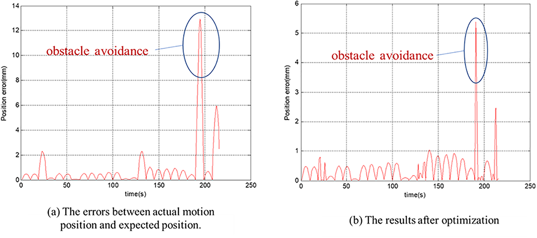
Trajectory error: (a) the errors between actual motion position and expected position and (b) the results after optimization.

Figure 16.

Trajectory planning process of redundant manipulator.

Figure 17.

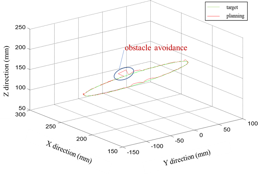
Comparison of target trajectory with planning trajectory of manipulator’s end effector.

Figure 18.

The velocity curve of each joint using velocity distribution of configuration plane method.

Conclusions

In this article, for the sake of concentrating on trajectory planning of redundant manipulator research issues, a trajectory planning method based on the configuration plane velocity distribution was proposed, and conclusions were summarized as follows:

A summary of the characteristics of the configuration plane which consists of the serial manipulator is provided. Furthermore, the definition of the configuration plane was put forward, and the basic kinematics model of which was established. Then, the method of velocity distribution based on configuration plane was derived, which lay the foundation for the trajectory planning of redundant manipulators.

To satisfy the spatial constraints during spatial motion process of the manipulator, the rational work configuration could be quickly obtained using the configuration plane method proposed in the article, which was concise and explicit. Furthermore, compared with the numerical methods, such as GA and iterative algorithm, the configuration plane method proposed in the article had the following advantages. Firstly, the calculation amount is greatly reduced. Secondly, the configuration plane method had generality for the majority of various redundant manipulators.

Furthermore, to resolve the problem that the motion trajectory between interpolation points is incontinuous and uncontrollable during the motion process of the manipulator, the velocity distribution based on configuration plane method was proposed. This method utilized the smoothing characteristics of the linear velocity of the manipulator’s end effector within a short period of time to ensure the continuity of motion. Simultaneously, to avoid spatial interference between the manipulator and obstacles, the velocity distribution was conducted for some joints in the configuration plane which were close to the obstacle. In addition, the controllability of the redundant manipulator in the trajectory between interpolation points was strengthened. Finally, through the trajectory planning simulation experiments of the redundant manipulator with 7 DOFs, the controllability and continuity of the end effector trajectory of the redundant manipulator are effectively enhanced. Compared with the common method, the method proposed in this article can not only improve the control accuracy of the manipulator by six to nine times in the case of obstacles but also greatly smooth the motion trajectory of the manipulator, which is able to be applied in a host of industrial tasks such as welding and grabbing.