Sage Journals: Discover world-class research

Abstract

This article presents an optimization technique to develop minimum energy consumption trajectories for redundant/hyper-redundant manipulators with predefined kinematic and dynamic constraints. The optimization technique presents and combines two novel methods for trajectory optimization. In the first method, the system’s kinematic and dynamic constraints are handled in a sequential manner within the cost function to avoid running the inverse dynamics when the constraints are not satisfied. Thus, the complexity and computational effort of the optimization algorithm is significantly reduced. For the second method, a novel virtual link concept is introduced to replace all the redundant links to eliminate physical impossible configurations before running the inverse dynamic model for the trajectory optimization. The method is verified on a three-degree of freedom redundant manipulator and the result is also demonstrated with computer simulations based on an 8-link planar hyper-redundant manipulator.

Keywords

Optimum trajectory planning energy minimization constraint handling cost function redundant manipulators hyper-redundant manipulator virtual link

Introduction

Although the nonredundant commercial robot’s performance and capability provide significant advantages for industrial implementations, however, in today’s modern industrial world consist of multitask industrial issues. The requirements of industrial applications are vastly complex and difficult, and these applications demand better performance and flexibility, such as drilling, cutting, medical robotics, maintenance of nuclear reactors, and so on. In order to meet these demands, robotic manipulators may have more degrees of freedom (DOFs) than essential due to execute intended complicated jobs like human arms. The extra DOFs can be named redundant, and redundancy mainly aims at increasing the robotic manipulator’s dexterity.

Research on redundant robotic manipulator is still active and redundancy can also be utilized to handle other cost criteria effectively. For example, redundancy has been used to achieve collision avoidance in working space,^1,2 preventing singularities where the manipulator lose some DOFs,^3,4 avoiding limits of joints,^5,6 minimizing some cost function such as reducing jerk^7,8 and torque,⁹ reducing deviation of the end effectors,^10,11 and reducing time¹² over a intended task. Redundancy can also be exploited for fault tolerance during the intended task.^13

–16 Redundancy also provides a larger orientation workspace and higher stiffness.^17,18 In addition to these, energy consumption can be reduced by utilizing redundancy¹⁹ in trajectory optimization. For example, a cost function was formulated by the input electrical energy/power and trajectory deviation for a redundant manipulator.²⁰ In other study, a full linear electromechanical model is used to minimize energy consumption.²¹ Displacement limits are included in the optimization algorithm via penalty functions. Redundant actuation can also reduce the energy consumption of parallel mechanisms with a considerable margin. In the study by Lee et al.,²² a widely used 2-DOF parallel mechanism design driven by three actuators is used to reduce the energy consumptions. In the study by Doan et al.,²³ an optimal redundancy resolution approach for a 6-DOF articulated welding robot is presented to reduce energy consumption while meeting the process requirements and satisfying all the kinematic constraints. In this study, the parameterized inverse kinematics in position domain and a modified particle swarm optimization were combined, hence an efficient redundancy resolution is realized. In the study by Li et al.,²⁴ for overcoming the singularity problem arising in the control of manipulators, redundancy resolution is also used to maximize manipulability under nonlinear constraint equations. A dynamic neural network for recurrent calculation of manipulability-maximal control actions for redundant manipulators under physical constraints in an inverse-free manner is presented.

In a fully actuated system, inverse kinematic solution of nonredundant robotic manipulators generally offers minimal numerical computational complexity, and the number of control inputs is equal to the DOFs of the system. However, in the redundant case, inverse kinematic solutions and control of the redundant link become more and more complicated and trajectory optimization problem also become increasingly difficult with each added redundant DOF.²⁵ Because, the utilized trajectory optimization algorithm can be numerically and computationally extremely complex and challenging issue due to the large number of optimization parameters and various constraints which need to be handled effectively during the optimization process of the computationally intensive inverse dynamic model. Moreover, the success of any optimization procedure, the trajectory optimization algorithm should be easily used on various types of nonredundant, redundant, and hyper-redundant manipulators, and the various types of constraint equations should be handled effectively during the trajectory optimization procedure. To determine the optimum solution successfully for trajectory optimization in redundant case, computationally efficient optimization procedures are preferred for a given task.

This article presents a novel constraint handling method and an efficient control algorithm for trajectory optimization to prevent the computational complexity of the redundant and hyper-redundant manipulators. One of the main contributions of this article is to provide constraint handling procedure is computationally efficient as kinematic and dynamic constraints are included in the cost function to prevent running inverse dynamic model when all constraints are not satisfied. Thus, the complexity and computational effort of the optimization algorithm is significantly reduced. And second contribution of this article, all the redundant links are acting as a single link. Hence, it makes controlling these links easier and control complexity of the redundant/hyper-redundant manipulators is reduced. This control algorithm prevents inverse dynamic failure even if the manipulator is within the workspace during the optimization process. The effectiveness of the proposed methods is initially demonstrated using computer simulations, and then same intended trajectories are implemented experimentally by utilizing the Katana 450 6M industrial robotic manipulators based on links 2, 3, and 4. In addition to the Katana 450, the effectiveness of the proposed methods is additionally demonstrated experimentally by utilizing the Denso VP-6242G industrial robotic manipulator based on links 2, 3, and 4. The proposed scheme is also verified with computer simulations based on an 8-link planar hyper-redundant manipulator.

The organization of the rest of the article can be summarized as follows. The system description and dynamics, the procedure of optimum trajectory planning, have been presented in second section. The proposed method has been shown in third section. The experimental implementation and results have been illustrated in fourth section.

System description and dynamics

Figure 1 shows the 6-DOFs of the Katana 450 robotic manipulators with end effector tool. It consists of 6-DOFs propelled by six DC motors with incremental encoder controlled by independent axis controller hardware. Gears are harmonic drive. The Katana 450 manipulator has an internal control box, which is directly mounted on the robot’s foot. The supply voltage is 24VDC and average energy consumption is approximately 50 W. The main board has PPCMPC5200 processor of 400 MHz, 32 MB Flash, and 64 MB RAM. Operating system is embedded GNU/Linux. Carrying load capacity is approximately 400 g. Dynamic modeling of the robot is based on Lagrangian dynamics, which describes the system in terms of its energy. To construct the inverse dynamic model of the system, the DYSIM software is utilized and it will operate from within the MATLAB/Simulink environment. DYSIM requires the user to specify the mass, inertia, and position of center of mass for each link, as well as identifying the location of ground point. The origin of the coordinate system is located at the point where the rotary axis of actuator 2 lier in Figure 1. The y represents the rotary axis of actuator 2, 3, and 4, respectively. A pictorial example of the definition of link 2 is connected to the actuator base 2, which is connected to the ground (defined as base). The maximum reachable point of the manipulator is approximately 0.6024 m from the actuator 2 base point. Links 2, 3, and 4 of the Katana manipulator (rotary joints 2, 3 and 4) are considered for the implementation of three-link redundant manipulator. In this implementation, the base of the manipulator and rotary joints of links 5 and 6 are locked at 0° relative angles during the redundant implementation. In this case, a system has more control inputs than required in order to control a specified desired motion. That is, the robotic manipulator has 3-DOFs, but the planar system has 2-DOFs. In this case, the inverse dynamic equations consists of more unknowns than the number of equations. For the redundant scheme, the manipulator task consists of transporting a load mass of 0.3 kg from an initial point at $(x_{i} = - 0.3095, y_{i} = 0.4881)$ m to a destination at $(x_{f} = 0.1405, y_{f} = 0.4381)$ m in Cartesian space as shown in Figure 1. It can be seen from the Figure 1 that the first link of the manipulator has redundancy, and the rest of the links are nonredundant. The total duration of motion is varied from 4 to 10 s by increments of 2 s. The DYSIM program selects 11 generalized coordinates (three for each links and two for the load) for the robotic manipulator as follows

q = [x_{1}, y_{1}, θ_{1}, x_{2}, y_{2}, θ_{2}, x_{3}, y_{3}, θ_{3}, x_{L}, y_{L}]

where x_i, y_i, and θ_i are the Cartesian coordinates of center of gravity and the joint angle, respectively, for link i. The system consists of 20 constraints and 23 variables. The DYSIM program automatically develops the Lagrangian function, the dynamic equations of motion including constraint equations and differential–algebraic equations. The initial conditions of the dependent coordinates based on the user-defined initial position conditions of the user-selected three independent coordinates and angle of θ₁, θ₂, and θ₃ are also automatically calculated by the DYSIM program. In this case, θ₁, x_L, and y_L were selected as the motion-defining independent variables. All the theoretical simulations for three-link redundant robotic manipulators are also executed experimentally on the Katana 450 robotic manipulator. The experimental data from the Katana 450 axes were recorded as raw data such as encoder position, encoder velocity, and encoder time, and then this recorded data are analyzed and converted to angles in degrees to compare with the demand and actual trajectories.

Figure 1.

Katana model with one redundancy in link 2.

The procedure of optimum trajectory planning

Formulation of the optimization problem and definition of the trajectory

Assumed that the n-links redundant manipulator task consists of transporting a load mass, m_load, from an initial point, P_initial, to a destination, P_final, in Cartesian space in Figure 2. Cartesian coordinates of the center of gravity and the relative angles of each link plus the Cartesian coordinates of the load are selected as generalized coordinates, that is, a total of (3n + 2) generalized coordinates for the n-DOF system. DYSIM automatically develops (2n + 2) constraint equations and a constraint Jacobian matrix F. For the formulation of the inverse dynamic model, the parametric desired motion for this n-DOF system is specified by using the Cartesian coordinates of the end effector (f_x and f_y), and the first (n − 2) relative angles of the redundant manipulator ( $θ_{i}, i = 1 \dots n - 2$ ). The last two relative angles (θ_{n − 1} and θ_n) are selected as dependant coordinates. The n control input locations are selected to be the relative angles of all n links (i.e. the joint actuator torques). To construct the trajectory, the uniform fifth-order B-spline function utilized and it consists of five segments, and each segment is a polynomial function with a maximum degree of four. A fifth-order B-spline function with five sections requires nine control points, r₁ to r₉. Three control points (r₂, r₃, and r₄) were utilized to satisfy the initial conditions (position, its first and second derivatives) and the other three control points (r₇, r₈, and r₉) were used to satisfy the end conditions (position, its first and second derivatives). The remaining three free control points (r₁, r₅, and r₆) are optimized by the optimization algorithm. As a result of this, six free parameters for the trajectory of the end effector in Cartesian coordinates (f_x(t) and f_y(t)) and four free parameters for the relative angle of each redundant links are used by the optimization algorithm. In the case of redundant manipulators, the end position of the redundant links is also to be optimized and not known in advance. In order to start the optimization algorithm, initial values of the free parameters have to be specified. Arbitrary selection of the free parameters is used for the initial trajectory in the optimization algorithm for the redundant/hyper-redundant manipulators. The velocity and acceleration profiles are zero at the initial and final positions. In order to implement the optimized trajectory experimentally, optimized fifth-order B-spline trajectory has to be converted to cubic polynomials due to input requirements of experimental implementation on Katana manipulator.

Figure 2.

Schematic view of a redundant manipulator. Last two links are nonredundant.

Cost function

G represents the cost (objective) between initial and final postures

G = \int_{0}^{T} (\sum_{i = 1}^{K} g_{i}^{2} (t)) d t

where g_i is the required actuator torque to be applied at joint i, and T is the motion duration. Calculation of the cost function in equation (2) requires the running of the inverse dynamic model for T s.

Proposed methods

Proposed penalty algorithm and optimization

The cost function calculations involve running the computationally intensive inverse dynamic model, which is time consuming. In conventional methods (such as the fmincon function in MATLAB), the constraints equations are handled separately as it is seen from Figure 3(1) and the cost function is called regardless of whether the constraints are satisfied or not. In order to improve computational efficiency of the trajectory optimization algorithm, constraints can be handled within the cost function calculations as seen in Figure 3(2). The proposed approach involves running the optimization without the conventional constraint functions and checking the constraints within the cost function before calling the inverse dynamic simulation. This way, the inverse dynamic analysis is only evaluated when these constraints are satisfied. The proposed penalty algorithm procedure is summarized as follows:

A global variable p is created (the initial values of p is set to zero) to count the number of cost function calls where the parameters do not satisfy the constraint equations.

During the cost function call, if the constraints are satisfied, the cost value is calculated by calling the inverse dynamic program in accordance with equation (2).

If any of the constraints are not satisfied, an alternative cost value is returned without running the inverse dynamic model as follows

p = p + 1 and G = b b (1 + p / 10)

where bb is a large base value and is set to $b b {= 10}^{5}$ . Equation (3) will ensure that the alternative cost value will be always updated and increased at each violation of the constraints to avoid a local minimum to be found outside of the constraints. The automatic update of alternative cost value for each cost function call outside the constraints (independent of the severity of violation) does not distort the original cost function of the trajectory optimization algorithm, instead it has an effect of avoiding some constraints to be treated as more important than others in the optimization algorithm. The value of bb is kept constant during the trajectory optimization process. In theory, this value can be fixed to any arbitrary value, however, in practice, the performance of an optimization algorithm will be depended on the selection of the value of bb. The value of bb should be higher than the worse case cost function value when constraints are satisfied. Therefore, a value of bb set to $b b {= 10}^{5}$ (after some trial and experiments) is selected for this study.

Figure 3.

(1) Conventional optimization method, constraints are handled as nonlinear inequalities in the constraint function; (2) proposed optimization method, constraints are handled in the cost function.

Proposed virtual link concept

In addition to kinematic constraints that may be imposed on the position, velocity, and acceleration profiles of each joint, it is crucial to ensure that the parametric trajectory functions generated by the trajectory optimization algorithm give a realizable motion within the workspace of the robotic manipulator. Otherwise, the inverse dynamic simulation will fail to run during the cost function calculation, and hence the optimization will fail. Because, redundant robotic manipulators may consist of any number of DOFs and any length. In this case, each of the redundant links has an infinite number of solutions for the desired end effector position. This situation can cause many problems when executing the optimization, such as the complexity in computational, long computations time, and difficulty in finding the optimal solution between the infinite numbers of solutions. However, this proposed virtual link concept has the capability to control a large number of DOFs manipulator while reducing the energy consumption in the optimization algorithm. Therefore, the distance between the end of the proposed virtual link (the last redundant link point at x_r, y_r) and the end effector (point at f_x, f_y) must be less than or equal to ( $l_{n - 1} + l_{n}$ ). In this case, the proposed virtual link will be checked by the proposed penalty algorithm in order to guarantee a realizable motion within the workspace envelop. In this instance, the proposed penalty algorithm and the proposed virtual link concept will be combined and run together in the trajectory optimization algorithm. This is equivalent to replacing the redundant links by a single virtual link R_rm as shown in Figure 2. At each step of the movement, the position of the redundant/hyper-redundant robotic manipulators has to satisfy the following constraint, which can be formulated as follows

R_{n r m} = max \sqrt{{(f_{x} - x_{r})}^{2} + {(f_{y} - y_{r})}^{2}} \leq l_{n - 1} + l_{n}

where x_r and y_r can be calculated from the optimization parameters as follows

x_{r} = \sum_{i = 1}^{n - 2} l_{i} cos θ_{i} and y_{r} = \sum_{i = 1}^{n - 2} l_{i} sin θ_{i}

The most important advantage of this proposed method is that whatever the length of the redundant links, it will always be acting as a virtual link (as a single link) (R_rm). Figure 4 demonstrates the simplified view of Figure 2, and it can be seen from the Figure 4, the control algorithm in equation (4) enables intersection of the two circles. This intersection point of two circles will be satisfied at each step of the movement. Hence, redundant links position on the workspace is guaranteed by a virtual link (R_rm) and computational complexity of the redundant/hyper-redundant links are significantly reduced. In addition to the kinematic and dynamic constraints, this nonlinear constraint ensures the end effector is on a reachable point in Cartesian coordinates. In this criterion, the distance between the origin and end effector must be less than the sum of all of the link lengths. The following criterion must satisfy the end effectors reachable point R_eef in Cartesian coordinates

R_{e e f} = max \sqrt{(f_{x}^{2} (t) + f_{y}^{2} (t))} \leq \sum_{i = 1}^{n} l_{i}

for 0 ≤ t ≤ T. Since f_x and f_y are generated from the optimization parameters, this constraint can also be checked before calling the inverse dynamics. The solution of the optimization problem is obtained using sequential quadratic programming techniques (such as the “fmincon” function in MATLAB. The steps of our proposed energy minimization algorithm based on inverse dynamic are shown in Figure 5 and detail can be found as follow:

Before executing the optimization algorithm, all kinematic and dynamic constraints of the mechanism have to be identified. In this example, these constraints are based on maximum and minimum values of the position, velocity, acceleration, torque values, and end effector reachable point R_eef in equation (6) and R_nrm in equation (4).

Hereafter, optimization algorithm will begin from suitable and feasible initial conditions (randomly for redundant/hyper-redundant case) for a given initial and final position in the desired coordinate system and the duration of motion.

Before the cost function calculation algorithm runs inverse dynamic program, it will check the kinematic constraints boundary conditions such as position, velocity, and acceleration profile and also end effector reachable point R_eef in equation (6) and R_nrm in equation (4) of the system. In this step of the algorithm, two situations can occur:

If the kinematic constraints are not satisfied and have violated the boundary conditions, the inverse dynamic analysis will not run. Therefore, these kinematic boundary conditions in the cost function will be punished heavily by utilizing proposed penalty algorithm (as in equation (3)). After all this, the optimization algorithm will go back to step 2 in order to find minimum cost value in the system.

If the kinematic constraints are satisfied, inverse dynamic programming will be run in order to calculate the dynamic cost function. In this case, two situations can also occur: If the torque limitations or other dynamic constraints are violated, the dynamic constraint equation will also be punished by proposed penalty algorithm. Hence, the optimization algorithm will continue with step 2. In other cases, if the torque limitation is satisfied, cost value of the system will be calculated by the inverse DYSIM dynamic program. The output of the inverse dynamic will be the new cost value of the system.

This procedure will continue until the optimization algorithm finds the lowest cost value. The procedure of the optimization algorithm and also the proposed penalty algorithm are shown in Figure 5.

Figure 4.

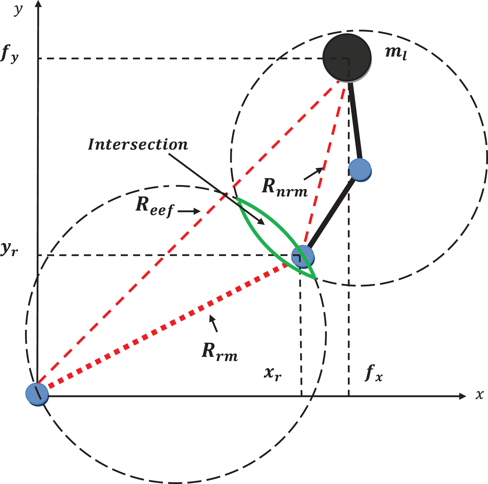
Simplified model of the virtual link in Figure 2.

Figure 5.

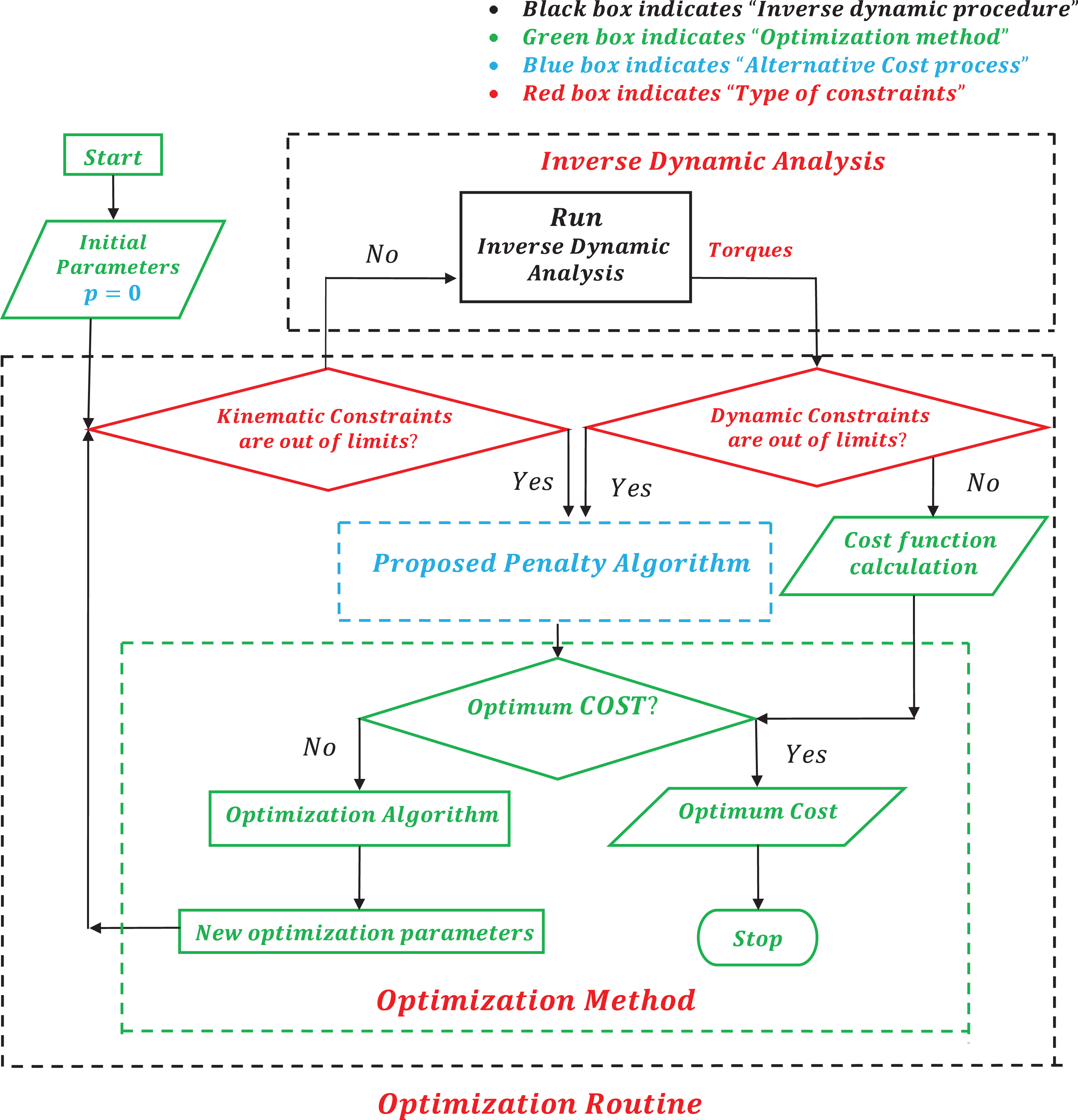
Proposed optimization procedure.

Experimental implementation and results

Optimum trajectory planning for three-link redundant manipulator on Cartesian coordinate

The proposed methods were implemented in Simulink. All these required parameters are summarized in Table 1. Figure 6 shows the corresponding optimized manipulative task with varying durations of motion in temporal trajectory position. The temporal positions in this figure clearly show us the manipulator’s behaviour during the simulations. It can be seen from the figure that the robotic manipulator has followed different paths for each duration of motion without violating the kinematic and dynamic constraint conditions. Figure 7 shows the output determinant of the augmented matrix for varying durations of optimum motion of redundant trajectories. This determinant is a good candidate to indicate a singularity point of the resulting trajectories. In Figure 7, while approaching a singularity point at t = 1.1 s, t = 1.55 s, t = 2 s, and t = 2.65 s, for the durations of motion of t = 2 s, t = 4 s, t = 6 s, and t = 8 s, respectively, the determinants of the redundant manipulator become zero indicating singularity configurations. At these singularity points, relative angles of link 4 to the link 3 of the robotic manipulators are almost 0° as indicated in the red-colour link as shown in Figure 7. However, the current robotic configurations allow the robotic manipulator to move away from singularity point and it quickly recovers from such a situation without stopping or/and stucking in a singular point during the desired motion. Although a smoothness of passing through singularity points is not guaranteed completely, all of the determinants changed their signs around the singularity points and motion continued. Figure 8 presents the comparison between the theoretically simulated optimized velocity profiles (reference) and the experimentally recorded optimized velocity profiles (actual) for links 2, 3, and 4, respectively. The velocities do not violate the velocity constraints. As expected, experimental results of the velocities support the simulation results, and the identical velocity profiles between the demand and actual velocity have been observed. As it can be seen from the velocity profile for 4 s, the link 2 is the slowest link among the other two links. In this duration of the motion, the robotic manipulator attempts to move the link 3 and link 4 away rapidly from the initial point, and this movement results in a high velocity profile for the link 3 and link 4 during that motion. While approaching a singular point at 1.1 s (as shown in output determinant for 4-s motion in Figure 7), there is a sudden and sharp decline in the velocity profiles of link 3 and link 4. At a singular point at 1.1 s, the speeds of the link 3 and link 4 reach almost zero velocity for this duration of motion. In addition to this, link 2 becomes perpendicular to the x coordinate as shown in “temporal for 4 s” profile as shown in Figure 7. This duration of motion is also demonstrated in the actuator torque profiles as in Figure 9, which shows the theoretical comparison of variation of torque requirements with various durations of motion for the optimal redundant trajectories. As a result of this, a sudden decrease in the torque profile of link 2 is observed at 0.26 normalized time as shown in Figure 9 and it reaches zero torque magnitude at this duration of motion. After 0.4 normalized seconds, link 2 is taking the position almost vertical to the x axis, therefore it has an almost zero torque magnitude until the end of the simulation. Furthermore, the duration of the motion of 6 s has almost the same velocity and determinant profiles as the duration of motion of 4 s during the given task. As is seen from the velocity profile of 6 s of motion in Figure 8, they are inherently slower than the velocity profile of 4 s. In the duration of motion of 6 s, the velocity profiles of the link 3 and link 4 also have a sudden and sharp decline before they reach the 1.55 s of simulation time. Similar to the velocity profile of 4 s motion, in the duration of motion at 1.55 s, the velocity profiles of the link 3 and link 4 becomes almost zero. Similarly, in this singular configuration of the motion, link 4 is in the zero angle position relative to the link 3. In this duration of motion, the required torque profile is decreasing, and the necessary torque profile of 6-s motion is clearly less than the duration of motion of 4-s profile. Correspondingly, link 2 also takes the position as perpendicular to the x axis between the 0.4 and 1 normalized second of the torque profile of 6-s motion. Hence, the torque magnitude of link 2 has almost zero magnitude between these normalized times until the end of the desired motion. In the duration of motion of 8-s profile, unlike other movements in 4, 6, and 10 s, there are nearly two singular configuration points at 2 and 4.15 s of the motion. The corresponding manipulator’s configurations at these durations of motion are shown in “temporal position for 8 s” profile as shown in Figure 7. In the first singular point of the duration (at 2 s of motion), unlike other decline velocity curve profiles in 4, 6, and 10 s of the motion, it is quite sudden and sharper. In the duration of motion of 4.15 s, another singularity point occurs as shown in the output determinant for 8-s motion profile in Figure 7. For this duration of motion, the velocity profiles of link 3 and link 4 are once again approaching 0° as shown in the velocity profile for 8 s in Figure 8. In the second singular configuration of the manipulator, all of the torque profiles of the manipulator have been observed as zero torque magnitude for a short period of time as shown in Figure 9. The duration of the motion of 10-s profile indicates that the singularity point has occurred at the duration of motion of 2.65 s. Similar to the other movements, the velocity profile of link 3 and link 4 is approaching zero velocity at this duration of motion as shown in velocity profile for 10 s in Figure 8. In addition, the torque profile of link 3 and link 4 have a much smoother and lower torque magnitude among the others as shown in Figure 9. The recorded optimum current profiles of the various durations of motion of the experimental results are shown in Figure 9. In order to calculate the optimum current profile for each duration of motion, the experimental trajectories were carried out five times, and the current required in each of the actuators was recorded five times and averaged for each sampling of the simulation time. The optimum initial required current profile of link 3 is high and about 300 mA. Furthermore, the optimum initial required current profile of link 4 is also high and starting from 100 mA. If we compare these values with the values of optimum initial torque requirements of link 3 and link 4 in Figure 9, the comparison will clearly show us the experimental results which strongly support the theoretical outcomes.

Table 1.

Parameters for Katana 450.

	Link 2	Link 3	Link 4
Parameters
Mass of link (kg)	1.022	0.882	0.969
Length of link (mm)	190	139	273.4
Distance from CoG to end link (mm)	95	35.3	163.4
Inertia of link (kg·m²)	0.0445	0.0445	0.0114
Friction coefficient of link (N·ms/rad)	1.8	1.5	0.39
Mass of gear (kg)	0.233	0.233	0.182
Gear ratio	371	371	100
Limits
Absolute angle (deg)	132°	245°	224°
Relative angle (deg)	+102°/−30°	+/−122.5°	+/−112°
Max velocity (deg/s)	72.52	73.53	136.8
Max acceleration (deg/s³)	2321	2353	4378
Torque (N·m)	17	13	9

Figure 6.

Initial non-optimum path, tracking performance between reference path, and experimental output.

Figure 7.

Three-link redundant manipulator positions for the singularity points of the output determinants with varying durations of motion.

Figure 8.

Experimental comparison of speed with varying duration of motion.

Figure 9.

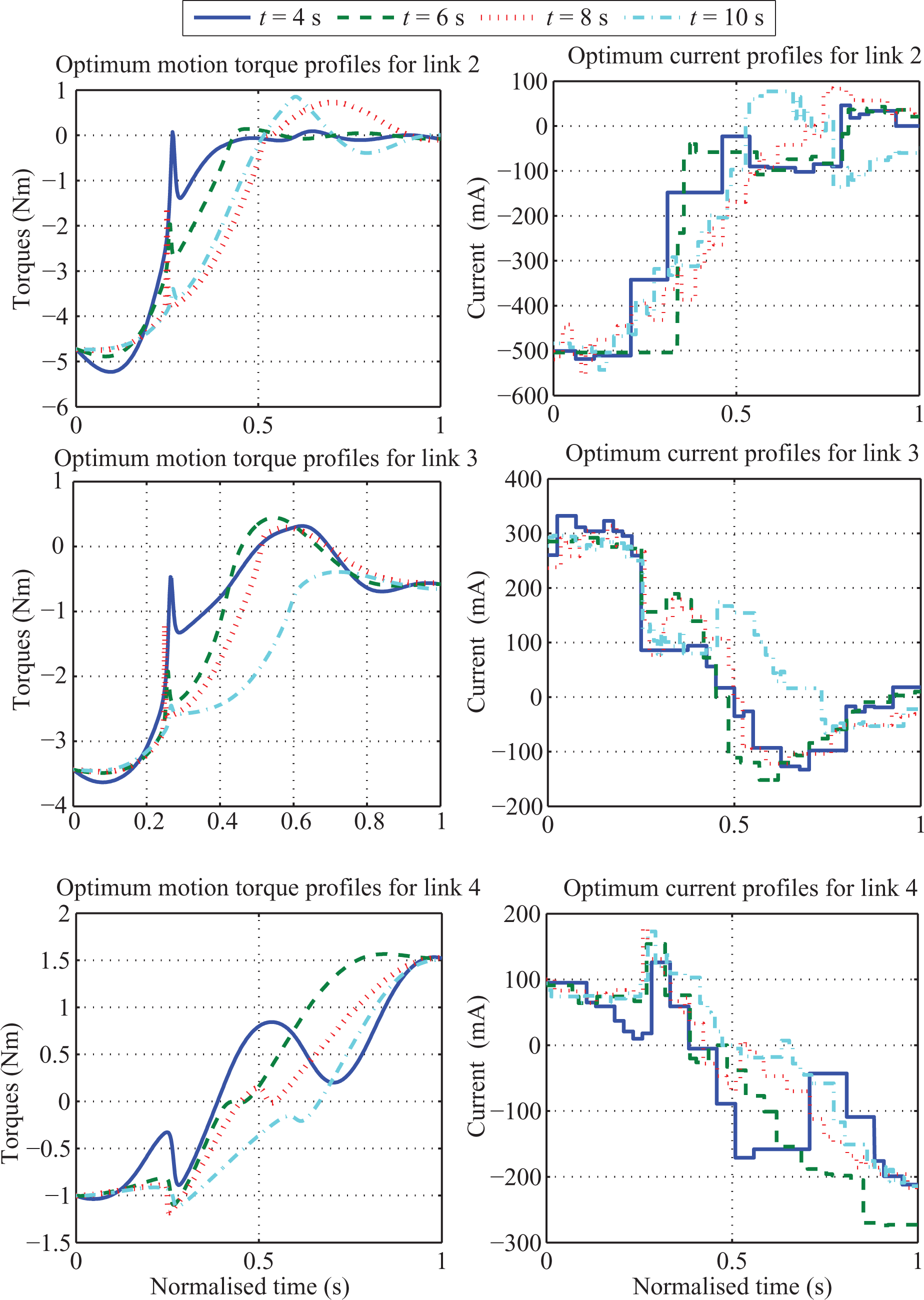
Comparison between simulated planned trajectories with torque and experimental current profiles.

As expected, the motion duration has a significant impact on the outcome of the cost function. It can be seen from the Table 2 that as the time of the motion is increased, the energy consumption is increased. After optimization, the cost value is reduced remarkably, and the considerable improvement achieved approximately 56.57% in 4-s motion in theoretical study. The corresponding experimental cost values for varying durations of motions are also demonstrated in Table 2 and maximum energy reduction was observed to be approximately 43.001%, which corresponds to the duration of motion of 4-s profile in the experimental study.

Table 2.

Cost values for Katana robot.

Time	Non-optimum	Optimum	Energy saving
Simulation	N²m²s	N²m²s	%
Cost (4 s)	87	38	56.57%
Cost (6 s)	128	62	51.48%
Cost (8 s)	169	92	45.78%
Cost (10 s)	211	122	42.21%
Experimental	amp²s	amp²s	%
Cost (4 s)	72	31	43.001%
Cost (6 s)	99	60	39.22%
Cost (8 s)	144	92	36.21%
Cost (10 s)	176	119	32.54%

In addition to the Katana 450 manipulator, the effectiveness of the proposed methods is also demonstrated experimentally by utilizing the Denso VP-6242G industrial robotic manipulator based on links 2, 3, and 4. For the Denso VP-6242G manipulator, it has an external control box, which is developed by Quanser company. The custom-designed controller box contains six amplifiers and built-in FF+PID (feedforward, proportional, integral, derivative) controllers. Carrying load capacity is approximately 2000 g. Dynamic modeling of the robots is also based on Lagrangian dynamics, which describes the system in terms of its energy. To construct the inverse dynamic model of the systems, the DYSIM software is utilized. The maximum reachable point of the manipulator is approximately 0.6844 m from the actuator 2 base point.

Link 2, 3, and 4 of the Denso manipulator (rotary joints 2, 3, and 4) are considered for the implementation of three-link redundant manipulator. For the redundant scheme, the manipulator task consists of transporting a load mass of 0.45 kg from an initial point at $(x_{i} = - 0.4185, y_{i} = 0.5945)$ m to a destination at $(x_{f} = 0.3285, y_{f} = 0.3935)$ m in Cartesian space as shown in Figure 10. The proposed methods were implemented in Simulink. All required parameters of the Denso are also summarized in Table 3.

Figure 10.

Denso model with one redundancy in link 2.

Table 3.

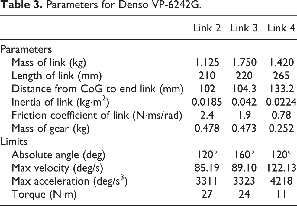
Parameters for Denso VP-6242G.

	Link 2	Link 3	Link 4
Parameters
Mass of link (kg)	1.125	1.750	1.420
Length of link (mm)	210	220	265
Distance from CoG to end link (mm)	102	104.3	133.2
Inertia of link (kg·m²)	0.0185	0.042	0.0224
Friction coefficient of link (N·ms/rad)	2.4	1.9	0.78
Mass of gear (kg)	0.478	0.473	0.252
Limits
Absolute angle (deg)	120°	160°	120°
Max velocity (deg/s)	85.19	89.10	122.13
Max acceleration (deg/s³)	3311	3323	4218
Torque (N·m)	27	24	11

It can be seen from the Table 4 that as the time of the motion is increased, the energy consumption is increased. After optimization, the cost value is reduced remarkably, and the considerable improvement achieved approximately 48.33% in 4-s motion in theoretical study. The corresponding experimental cost values for varying durations of motions are also demonstrated in Table 4 and maximum energy reduction was observed to be approximately 40.19%, which corresponds to the duration of motion of 4-s profile in the experimental study.

Table 4.

Cost values for Denso robot.

Time	Non-optimum	Optimum	Energy saving
Simulation	N²m²s	N²m²s	%
Cost (4 s)	120	62	48.33%
Cost (6 s)	165	91	44.84%
Cost (8 s)	206	120	41.74%
Cost (10 s)	251	162	35.45%
Experimental	amp²s	amp²s	%
Cost (4 s)	102	61	40.19%
Cost (6 s)	129	83	35.65%
Cost (8 s)	153	105	31.37%
Cost (10 s)	204	143	29.90%

In order to evaluate the outputs observed above, it is clear that the robotic manipulator has a very wide working space because the system has a redundant structure. As a result of this, it is much easier to get rid of the singularity problems for each joint, therefore, the redundant structure appears to be quite robust to kind of these problems during the motion. In addition, due to the wide working space of the redundant/hyper-redundant structure, there will be a considerable decrease in the actuator torque profiles during the movement of the system, thus the energy consumed by the actuators is considerably reduced.

By introducing a virtual link concept, all the redundant links are acting as a single link and it leads to controlling these massive number of DOF’s robotic manipulator easier and control complexity of the redundant/hyper-redundant manipulators is reduced. If the robot is asked to go to the point where it cannot reach, this virtual link constraint prevents inverse dynamic failure during the optimization process. Because, a virtual link concept eliminates physically impossible configurations before running the inverse dynamic model. The benefit of preventing the inverse dynamic failure to avoid the user from restarting the failing program every time and leaving the optimization program to decide whether to run the program. In this case, the optimization algorithm will generate the new optimization parameter itself without user factor during the simulation. In addition to virtual link constraint, other constraints are also handled effectively within the cost function to avoid running the inverse dynamics when the constraints are not satisfied. Therefore, computational complexity is reduced by preventing the running of inverse dynamic analysis.

Optimum trajectory planning for hyper-redundant manipulators

An eight-link hyper-redundant (with 6-DOFs redundancy) manipulator is introduced to verify the proposed methods for a large number of links. The simulation is carried out by the program DYSIM. The manipulator task for this example is to move the load mass from an initial point P_initial (x_i = 1.54, y_i = 0.14) m to a final point P_final (x_f = 0, $y_{f} = - 0.85$ ) m in Cartesian space coordinate as shown in Figure 11. The viscous friction effects of the joints are also included with a coefficient of friction “0.6” Ns/m and gears are also taken into account with all gear ratios $R_{1 - 8} = 50$ . The motion duration is specified as T = 2 s. Mass center of gravity of the links are in the middle of each link and the load mass is $m_{load} = 0.3$ kg at the end of the last link. An eight-link hyper-redundant manipulator has eight identical links, and each link length is selected as 0.2 m. For each link, motor and link inertias were selected as 0.0001 kg·m² and 0.0025 kg·m², respectively. All the links have identical mass, $m_{1} = \dots = m_{8} = 0.5$ kg and each motor mass was selected as 0.2 kg. The angle, velocity, acceleration, and torque constraints are given in Table 5. The DYSIM program selects 26 generalized coordinates (three for each links and two for the load) for the robotic manipulator. The system consists of 50 constraints and 58 variables. The Lagrangian function and the dynamic equations of motion including constraint equations and differential–algebraic equations are automatically developed by the DYSIM program. The program also calculates the initial conditions of the dependent coordinates based on the user-defined initial position conditions of the user-selected eight independent coordinates and the angle of θ₁ to angle of θ₈. In this case, angles of links θ₁ to θ₆ and x_L, y_L were selected as the motion-defining variable. In this hyper-redundant scheme, θ₁ to θ₆ indicate the relative angle of the redundant links of the robotic manipulator. The corresponding randomly generated feasible non-optimum and optimum manipulative task are shown in temporal trajectory positions and also corresponding end effector’s (EEF’s) tracking trajectory as presented in Figure 11. As is seen from the Figure 11, the EEF tracking curve of the motion trajectory corresponding to non-optimum parameters has almost a straight-line trajectory apart from the beginning of the motion. This movement of the manipulator provides high torque magnitude and sudden ascension on the non-optimized torque curves for all actuators between the duration of 1.3 and 1.4 s in the simulation as shown with dashes in Figure 12. As is seen from the Figure 13, the non-optimum cost curve increases rapidly and gives an initial cost value of G = 8084. On the other hand, the EEF tracking curve of the motion trajectory corresponding to optimum parameters has a smooth EEF tracking profile as shown in Figure 11(d). This optimum motion of the manipulator provides admissible torque magnitude and avoids sudden increases in torque profile during the motion as shown in Figure 12. The corresponding optimized cost curve is increasing smoothly as shown in Figure 13 and less incline is observed on the curve of the cost value due to the optimum parameters. After optimization, the cost function is reduced to G = 5232, which corresponds to 35.3% reduction along the desired trajectory.

Figure 11.

(a) Motion trajectory corresponding to initial parameter values, (b) end effector’s trajectory corresponding to initial parameter values; (c) motion trajectory corresponding to optimum parameter values, (d) end effector’s trajectory corresponding to optimum parameter values.

Table 5.

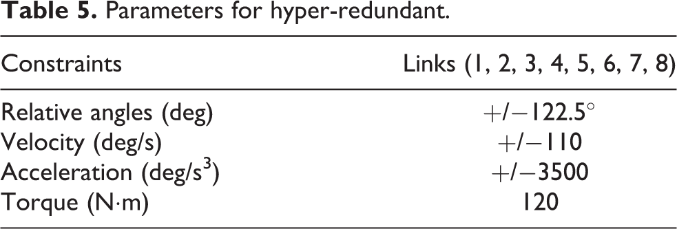
Parameters for hyper-redundant.

Constraints	Links (1, 2, 3, 4, 5, 6, 7, 8)
Relative angles (deg)	+/−122.5°
Velocity (deg/s)	+/−110
Acceleration (deg/s³)	+/−3500
Torque (N·m)	120

Figure 12.

Simulated planned trajectories of non-optimum and optimum torque profiles for hyper-redundant.

Figure 13.

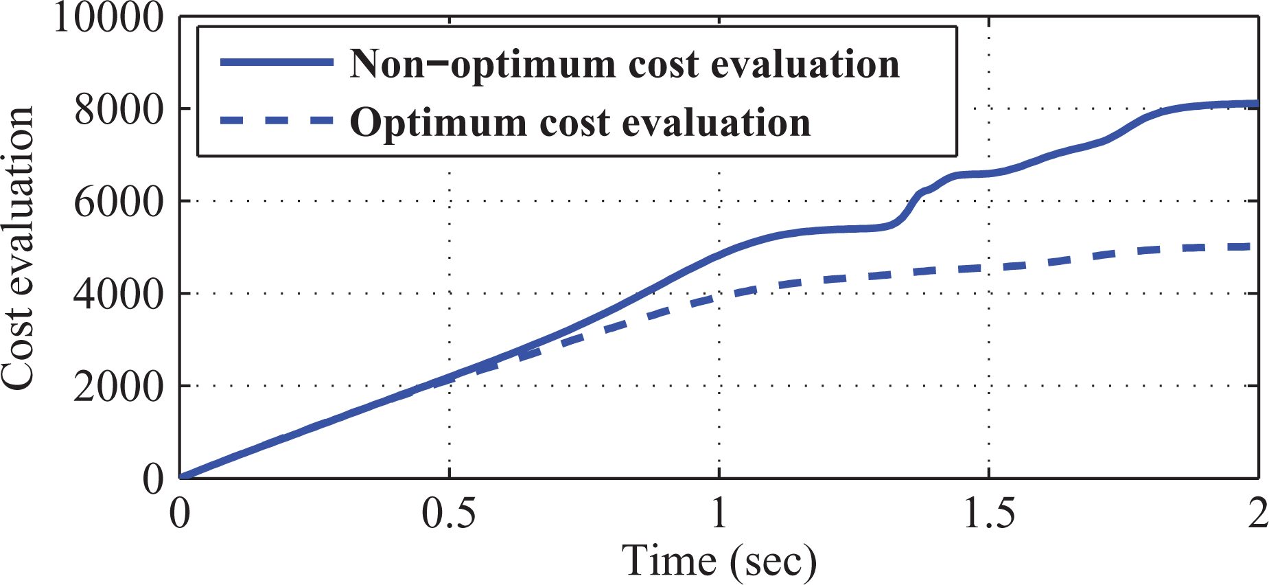
Cost evaluation of hyper-redundant robot.

Conclusion

The article has demonstrated experimentally efficient constraint handling technique and effective control algorithm to prevent running computationally intensive inverse dynamic model, when all constraints are not satisfied. The success of the proposed methods relies on the techniques that the kinematic and dynamic constraints are included in the cost function as well as introducing the virtual link concept, where all of the redundant links are acting as a single link during the motion. The simulation results make clear the effect of the proposed methods for the redundant/hyper-redundant robotic manipulators. The proposed methods not only achieve a reduction in the energy consumption for the hyper-redundant manipulators but also has the ability of handling a large number of DOFs manipulators and constraints without any problems. A variety of constraints and different cost functions can easily be added to the proposed optimization procedure.

Footnotes

Declaration of conflicting interests

The author(s) declared no potential conflicts of interest with respect to the research, authorship, and/or publication of this article.

Funding

The author(s) received no financial support for the research, authorship, and/or publication of this article.

References

Patel

Shadpey

Ranjbaran

. A collision-avoidance scheme for redundant manipulators: theory and experiments. J Robot Syst 2005; 22(12): 737–757.

Ping

Wei

. Real time obstacle avoidance for redundant robot. In: International conference on mechatronics and automation, Changchun, China, 9-12 August 2009, pp. 223–228. ICMA.

Duarte

FBM

Tenreiro Machado

(1999) A trajectory planning algorithm for redundant manipulators. In: Proceedings of the 1999 IEEE international symposium on assembly and task planning, 1999 (ISATP’99), Porto, Portugal, July 1999, pp. 175–180.

Huo

Baron

. The joint-limits and singularity avoidance in robotic welding. Ind Robot Int J 2008; 35(5): 456–464.

Assal

SFM

Watanabe

Izumi

. Intelligent control for avoiding the joint limits of redundant planar manipulators. Artif Life Robot 2006; 10(2): 141–148.

Mohammed

Chaumette

. New strategies for avoiding robot joint limits: application to visual servoing using a large projection operator. In: 2010 IEEE/RSJ international conference on intelligent robots and systems (IROS), Taipei, Taiwan, 18–22 October 2010, pp. 6222–6227.

Sullivan

JCW

Pipe

. Path planning for redundant robot manipulators: a global optimization approach using evolutionary search. In: 1998 IEEE international conference on, systems, man, and cybernetics, 1998, vol. 3, United Kingdom, 1998, pp. 2396–2400.

Yang

Kim

Pitarch

. Optimal trajectory planning for redundant manipulators based on minimum jerk. In: International design engineering technical conference and computer and information in engineering conference, 3–6 August 2008, pp. 1141–1150. Brooklyn, New York, USA: ASME.

Chen

Wang

. Design and dynamics of a novel solar tracker with parallel mechanism. IEEE-ASME Trans Mechatr 2016; 21(1): 88–97.

10.

Ata

Myo

. Optimal point-to-point trajectory tracking of redundant manipulators using generalized pattern search. International Journal of Advanced Robotic Systems, 2005; 2(3): 239–244.

11.

Singla

Tripathi

Rakesh

. Dimensional synthesis of kinematically redundant serial manipulators for cluttered environments. Robot Auton Syst 2010; 58(5): 585–595.

12.

Watanabe

. Minimum time path-tracking control of redundant manipulators. In: Proceedings. 2000 IEEE/RSJ international conference on intelligent robots and systems, 2000 (IROS 2000), vol. 1, USA, 31 October–5 November 2000, pp. 27–32.

13.

Yan

Yamamoto

Murakami

. Autonomous decentralized approach in the PTP control of redundant manipulators. In: 1998 5th international workshop on advanced motion control, 1998, AMC’98-Coimbra, Coimbra University, Coimbra, Portugal, 29 June–1 July 1998, pp. 153–158.

14.

Roberts

HG,

Maciejewski

. Fundamental limitations on designing optimally fault-tolerant redundant manipulators. IEEE Trans Robot 2008; 24(5): 1224–1237.

15.

Roberts

Siddiqui

SA,

Maciejewski

. Designing equally fault-tolerant configurations for kinematically redundant manipulators. In: 41st Southeastern symposium on system theory, University of Tennessee Space Institute Tullahoma, TN, USA, 15–17 March 2009, SSST, pp. 335–339.

16.

Soylu

Buckham

BJ,

Podhorodeski

. Redundancy resolution for underwater mobile manipulators. Ocean Eng 2010; 37(2): 325–343.

17.

Wang

. Dynamics and control of a planar 3-DOF parallel manipulator with actuation redundancy. Mech Mach Theory 2009; 44(4): 835–849.

18.

Wang

. Performance analysis and comparison of planar 3-DOF parallel manipulators with one and two additional branches. J Intell Robot Syst 2013; 72(1): 73–82.

19.

Halevi

Carpanzano

Montalbano

. Minimum energy control of redundant actuation machine tools. CIRP Ann Manuf Technol 2011; 60(1): 433–436.

20.

Hirakawa

Kawamura

. Trajectory planning of redundant manipulators for minimum energy consumption without matrix inversion. In: Proceedings., 1997 IEEE international conference on robotics and automation, Albuquerque, New Mexico, April 1997, vol. 3, pp. 2415–2420.

21.

Halevi

Carpanzano

Montalbano

. Minimum energy control of redundant linear manipulators. J Dyn Syst Meas Control 2014; 136: 051016–1.

22.

Lee

Jeong

. Minimizing energy consumption of parallel mechanisms via redundant actuation. IEEE/ASME Trans Mechatr 2015; 20(6): 2805–2812.

23.

Doan

NCN

Tao

Lin

. Optimal redundancy resolution for robotic arc welding using modified particle swarm optimization. In: 2016 IEEE international conference on advanced intelligent mechatronics (AIM), Banff, Alberta, Canada, 12–15 July 2016, pp. 554–559.

24.

LJS

Liuo

. Manipulability optimization of redundant manipulators using dynamic neural networks. IEEE Trans Ind Electr 2016; 64(6): 1–10.

25.

Dasgupta

Gupta

Singla

. A variational approach to path planning for hyper-redundant manipulators. Robot Auton Syst 2009; 57(2): 194–201.

Real time optimum trajectory generation for redundant/hyper-redundant serial industrial manipulators

Abstract

Keywords

Introduction

System description and dynamics

The procedure of optimum trajectory planning

Formulation of the optimization problem and definition of the trajectory

Cost function

Proposed methods

Proposed penalty algorithm and optimization

Proposed virtual link concept

Experimental implementation and results

Optimum trajectory planning for three-link redundant manipulator on Cartesian coordinate

Optimum trajectory planning for hyper-redundant manipulators

Conclusion

Footnotes

Declaration of conflicting interests

Funding

References