Sage Journals: Discover world-class research

Abstract

During high-speed pick-and-place operations, elastic deformations are quite apparent if the mass of the manipulator is low. These irregular deformations are accompanied by vibrations, then errors. Since elastic potential energy reflects elastic deformation, the vibration of the whole manipulator can be controlled well when the elastic potential energy is decreased. In this article, to design manipulators with flexible links for pick-and-place operations, an integrated structure and control design framework is proposed. The dynamic model of a coaxis planar parallel manipulator is obtained by the finite element method, an effective method. A proportional–derivative controller is utilized for this industrial application. Simultaneously, the optimal structural and control parameters are derived by minimizing the elastic potential energy via integrated design, in which actuated systems and accuracies are regarded as constraints. Finally, simulations show that the performance of the parallel manipulator is improved by this design methodology.

Keywords

Parallel manipulator dynamics integrated design pick-and-place coaxis

Introduction

Pick-and-place operations are needed in industries of electronics, pharmaceutics, foods, and so on. In these operations, manipulators must be complete the tasks in short-cycle time.¹ Dynamic performance, therefore, takes a critical role in manipulator evaluation and design. An effective way to increase acceleration is to reduce masses of moving parts. Yet it’s noteworthy that mass reduction will eventually cause obvious flexibility effects so that vibrations and errors of manipulators will become severe. Thus, elastic potential energy cannot be neglected in the dynamic analysis. In the conventional mechanical design process, structure design and control design are performed separately. This design process has been unable to achieve the demanding requirement in some modern industries. By optimizing structural parameters to suppress vibration, the natural frequency is a widely used index.^2
–4 To reduce vibrations of robot manipulators, many researchers have focused preferentially on control strategies. A popular study object is the single-link flexible manipulator system. Mohamed and Tokhi⁵ apply command shaping techniques based on input shaping, low-pass, and band-stop filtering for vibration control. Hassan et al.⁶ propose a model-based predictive controller for vibration suppression. A neural network controller is designed to eliminate the effects of the input dead zone of the actuators by He et al.⁷ Vibration control has also been studied for two-link flexible manipulators.^8,9,10 Since the coupled effects of structural and control parameters, Maghami et al.¹¹ have demonstrated the first attempt at an integrated structure and control design. The spacecraft design is improved by optimizing both structural and control parameters simultaneously. Then, this design methodology has been used for a four-bar manipulator by employing the simple proportional–derivative (PD) control,¹² a compliant two-axes mechanism to suppress vibration,¹³ a feed drive system to increase the system bandwidth and decrease Abbe offset,¹⁴ and a five-bar linkage manipulator to improve settling time,¹⁵ etc. It is not hard to see structures of the subjects in these studies that are simple, which have only less than three translation motions. And these studies are not about high-speed pick-and-place operations.

Lou et al.¹⁶ have presented a planar three-degree-of-freedom robot manipulator, which has three $R R R$ ( $R$ : revolute joint) subchain. This robot manipulator is called V3 (Figure 1), which has unlimited rotation capability. Similar structures have been presented by Isaksson¹⁷ in 2011. The kinematics and workspace of V3 robot have been analyzed in detail.¹⁸ To improve the velocity performance in workspace, the lengths of the links of the V3 robot have been optimized for pick-and-place operations. In this article, the integrated design methodology is utilized to further improve the 3T1 R parallel manipulator. In high-speed operation, the end-effector will be required not only to change the position but also the orientation in a surprisingly short time simultaneously. After reducing masses of moving parts, the horizontal flexibility increases conspicuously. In an early study,¹⁹ efficiency has been employed as the design objective, since the cycle time is a critical requirement for this industrial application. However, the elastic vibration was not controlled well. The elastic vibrations of links cannot be ignored, which may induce unstable motion of manipulator.^20,21 Thus, accuracy of manipulator is influenced by elastic deformation. To reduce adverse efforts and insure the whole performance, the integrated design methodology is an effective technique to improve the V3 robot system. For pick-and-place operations, a new general framework of the integrated structure and control design is presented in this article. The elastic potential energies of links are applied to characterize elastic vibrations, which are minimized to decrease the vibrations and also diminish the errors in this methodology. To simplify this problem, we just first consider the horizontal flexibility.

Figure 1.

The V3 robot: (a) 3D model and (b) side view. 3D: three-dimensional.

To begin with, a flexible-link robot system must be modeled. The elastodynamic model is required, which is characterized by nonlinear differential equations. Commonly, the assumed modes method (AMM) and finite element method (FEM) are the most frequently used methods to discretize the dynamic model.²² With dominant assumed modes for cantilever and pinned–pinned beams, the inverse dynamics model of flexible two-link manipulators has been studied by Green and Sasiadek.²³ A computationally efficient method based on the AMM for modeling flexible robots has been proposed by Celentano and Coppola.²⁴ To derive an appropriate low-order dynamic model for the design of the controller, Zhang et al.²⁵ have employed the AMM to discretize elastic motion of a rigid–flexible planar parallel manipulator. The AMM is also applied to achieve an n-dimensional discretized model of the two-link flexible manipulator for dynamic uncertainty analysis and controller design.²⁶ The FEM is widely used in modeling and analysis of robot manipulators as well. A relatively complicated case, a three- $P R R$ planar parallel manipulator, has been analyzed by using FEM.²⁷ The finite element model is presented for a unique approach for active vibration control of a one-link flexible manipulator.²⁸ And the finite element model is also applied to simulate the bending range of the central spring and static properties of a compliant gripper.²⁹ A comprehensive stiffness analysis method via finite element analysis has been obtained by Yu et al.³⁰ Both methods are effective to study elastodynamic model. However, for a manipulator with multilinks and irregular shapes, the AMM is not easy to achieve the model, while the FEM can be an effective alternative.³¹ With the AMM, it is usual to assume the modes of the links. If the shapes of the links are irregular, it is very hard to get the precise assumed modes. The model based on the FEM is composed of every element. No matter what the shapes of the links are, and they can be discretized into finite and regular elements. The model of the regular element can be precisely obtained. Thus, the manipulator with irregular shapes and multilinks is more easily modeled. In this article, we want to study a manipulator with variable cross-sectional links, so the FEM may be better suited for modeling.

The organization of this article is as follows. In the section “Dynamic modeling,” the V3 parallel manipulator system with flexible links is modeled by the FEM. In the section “Integrated design problem formulation,” the Lagrange multiplier is utilized to achieve the system dynamics with the loop-closure conditions. And a PD controller is employed in the integrated design problem which is regarded as an optimal design problem. Beginning with a regular example analysis, two-step integrated designs are put into effect. The computer simulations show the improvements of this system in section “Simulation and discussion.” In section “Comparison,” the results of conventional design are shown to compare with the results of integrated design. Conclusions are provided in the last section.

Dynamic modeling

This study supposes that all the links are only bent in the horizontal plane and other parts are rigid bodies. Referring to Figure 2, frame $O X Y Z$ is an inertial coordinate system, and point O is coincident with point A ₁ which is the center of the actuated joint in the subchain $A_{1} B_{1} C_{1}$ .

Figure 2.

(a) Inertial coordinate frame of the V3 robot and (b) the crank design.

Kinetic energy and potential energy

In Figure 3, there is a coordinate system to describe the ith flexible subchain. To facilitate the description of the robot system, the meanings of mathematical notations are proposed in Table 1. First, kinetic and potential energy of the parallel manipulator should be obtained, since the dynamic model will come from the Lagrangian formulation.

Figure 3.

The coordinate system of the ith flexible subchain.

Table 1.

Nomenclature.

Notations	Meaning
i	The subchain number ( $i = 1, 2, 3$ )
j	The link number of each subchain ( $j = 1, 2$ )
k	The element number ( $k = 1, 2, \dots, n_{i j}$ )
$O X Y$	The inertial coordinate frame
$o_{i j, k} x_{i j, k} y_{i j, k}$	The body coordinate frame attached to the kth
	Element of link ij
$l_{i j}$	Length of the jth link in the ith subchain
$l_{i j, k}$	Accumulated length of the first $(k - 1)$ elements
	On link ij
$a_{i j, k}$	Length of element k on link ij
$(x, y)$	Cartesian coordinate of point C ₁
$(x_{i}, y_{i})$	Cartesian coordinate of point C_i
$ϕ$	The included angle from $+ X$ direction to
	The vector $H_{1} H_{2}$
$θ_{i}$	The actuated angle variable of the ith subchain
$γ_{i}$	The angle variable between actuated link and
	Passive link of the ith subchain
b ₁	Length of the bar $H_{1} H_{2}$ in the crank
b ₂	Length of the bar $H_{3} H_{4}$ in the crank
$(u_{i j, k}, v_{i j, k})$	Flexural displace and slope of node k of link ij
$(u_{i j, e}, v_{i j, e})$	Flexural displace and slope at the end of link ij
$S_{i j, k}$	Cross-sectional area of the kth element on link ij
$ρ_{1}$ , $ρ_{2}$	Mass densities of actuated link and passive link

Suppose all the discretized elements on every link are Bernoulli–Euler beam, there are $n_{i 1}$ elements on the actuated link $i 1$ ( $A_{i} B_{i}$ ). Let’s consider a point P on the element between node k and $k + 1$ (element k). The vector $\overset{\leftarrow}{O P}$ is referred to as $p$ , which can be obtained as follow

p = [\begin{matrix} cos θ_{i} & - sin θ_{i} \\ sin θ_{i} & cos θ_{i} \end{matrix}] [\begin{matrix} l_{i 1, k} + x_{i 1, k} \\ y_{i 1, k} \end{matrix}]

where $(x_{i 1, k}, y_{i 1, k})$ are the coordinate of P with respect to the body frame $o_{i 1, k} x_{i 1, k} y_{i 1, k}$ . To achieve the coordinate $(l_{i 1, k} + x_{i 1, k})$ , the flexural deformation has been assumed to be very small. Then, the kinetic energy of the kth element can be calculated from the following integral

T_{i 1, k} = \frac{1}{2} ρ_{1} S_{i 1, k} \int_{0}^{a_{i 1, k}} {(\frac{d p}{d t})}^{T} \frac{d p}{d t} d x_{i 1, k}

Based on the FEM theory, the flexural displaces and slopes of nodes on both sides of the element k are utilized to approximate the displacement $y_{i 1, k}$

y_{i 1, k} = Ψ_{i 1, k}^{T} U_{i 1, k}

where $U_{i 1, k} = [θ_{i}, u_{i 1, k}, v_{i 1, k}, u_{i 1, k + 1}, v_{i 1, k + 1}]^{T}$ and $Ψ$ is the shape function matrix defined as follows

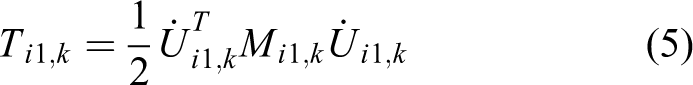
Ψ_{i 1, k} = [\begin{matrix} 0 \\ 1 - 3 x_{i 1, k}^{2} / a_{i 1, k}^{2} + 2 x_{i 1, k}^{3} / a_{i 1, k}^{3} \\ x_{i 1, k} - 2 x_{i 1, j}^{2} / a_{i 1, k} + x_{i 1, k}^{3} / a_{i 1, k}^{2} \\ 3 x_{i 1, k}^{2} / a_{i 1, k}^{2} - 2 x_{i 1, k}^{3} / a_{i 1, k}^{3} \\ - x_{i 1, k}^{2} / a_{i 1, k} + x_{i 1, k}^{3} / a_{i 1, k}^{2} \end{matrix}]

The kinetic energy of the kth element in (2) can be expressed according to the value of vector $U_{i 1, k}$ as the following form

T_{i 1, k} = \frac{1}{2} {\dot{U}}_{i 1, k}^{T} M_{i 1, k} {\dot{U}}_{i 1, k}

where $M_{i 1, k}$ is the element mass matrix, and it can be defined as

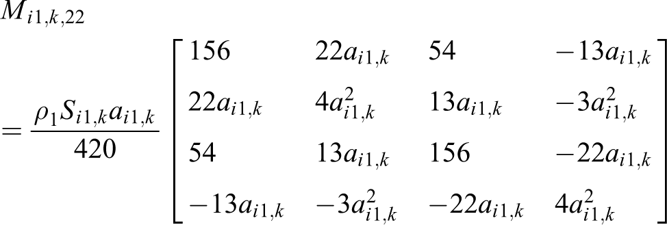
M_{i 1, k} = ρ_{1} S_{i 1, k} \int_{0}^{a_{i 1, k}} {(\frac{\partial p}{\partial U_{i 1, k}})}^{T} \frac{\partial p}{\partial U_{i 1, k}} d x_{i 1, k}

Clearly, $\partial p / \partial U_{i 1, k}$ is a $2 \times 5$ matrix. The $5 \times 5$ matrix $M_{i 1, k}$ is symmetric and can be partitioned as

M_{i 1, k} = [\begin{matrix} M_{i 1, k,11} & M_{i 1, k,12} \\ M_{i 1, k,21} & M_{i 1, k,22} \end{matrix}]

where

\begin{array}{l} M_{i 1, k,11} = ρ_{1} S_{i 1, k} (a_{i 1, k}^{3} / 3 + a_{i 1, k}^{2} l_{i 1, k} + a_{i 1, k} l_{i 1, k}^{2}) \\ + U_{i 1, k}^{T} [\begin{matrix} 0 & 0 \\ 0 & M_{i 1, k,22} \end{matrix}] U_{i 1, k} \end{array}

M_{i 1, k,12} = M_{i 1, k,21} = ρ_{1} S_{i 1, k} [\begin{matrix} 3 a_{i 1, k}^{2} / 20 + a_{i 1, k} l_{i 1, k} / 2 \\ a_{i 1, k}^{3} / 30 + a_{i 1, k}^{2} l_{i 1, k} / 12 \\ 7 a_{i 1, k}^{2} / 20 + a_{i 1, k} l_{i 1, k} / 2 \\ - l_{i 1, k}^{3} / 20 - a_{i 1, k}^{2} l_{i 1, k} / 12 \end{matrix}]

\begin{array}{l} M_{i 1, k,22} \\ = \frac{ρ_{1} S_{i 1, k} a_{i 1, k}}{420} [\begin{array}{l} 156 & 22 a_{i 1, k} & 54 & - 13 a_{i 1, k} \\ 22 a_{i 1, k} & 4 a_{i 1, k}^{2} & 13 a_{i 1, k} & - 3 a_{i 1, k}^{2} \\ 54 & 13 a_{i 1, k} & 156 & - 22 a_{i 1, k} \\ - 13 a_{i 1, k} & - 3 a_{i 1, k}^{2} & - 22 a_{i 1, k} & 4 a_{i 1, k}^{2} \end{array}] \end{array}

After investigating carefully, it is easy to find that $M_{i 1, k,12}$ , $M_{i 1, k,21}$ , and $M_{i 1, k,22}$ only depend on structural parameters and have nothing to do with flexural deformation and $θ_{i}$ . However, $M_{i 1, k,11}$ is a quadratic function of nodal displacement in the mass matrix.

The elastic potential energy is independent of the actuated angle $θ_{i}$ but only depends on the flexural displaces and slopes $(u_{i 1, k}, v_{i 1, k}, u_{i 1, k + 1}, v_{i 1, k + 1})$ . Therefore, the potential energy of the kth element can be obtained by

V_{i 1, k} = \frac{1}{2} U_{i 1, k}^{T} K_{i 1, k} U_{i 1, k}

where

K_{i 1, k} = [\begin{matrix} 0 & 0_{1 \times 4} \\ 0_{4 \times 1} & K_{i 1, k,22} \end{matrix}]

Here, $K_{i 1, k,22}$ is the basic stiffness matrix of beam element, which is frequently proposed in the FEM textbook.

The elements on link $i 2$ can be served following a similar approach. Let’s consider a point Q on the element between node k and $k + 1$ (element k). The vector $\overset{\leftarrow}{O Q}$ is referred to as q, which can be presented as follow

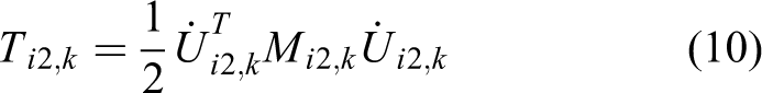
\begin{array}{l} q = [\begin{matrix} cos θ_{i} & - sin θ_{i} \\ sin θ_{i} & cos θ_{i} \end{matrix}] ([\begin{matrix} l_{i 1} \\ u_{i 1, e} \end{matrix}] \\ + [\begin{matrix} cos (γ_{i} + v_{i 1, e}) & - sin (γ_{i} + v_{i 1, e}) \\ sin (γ_{i} + v_{i 1, e}) & cos (γ_{i} + v_{i 1, e}) \end{matrix}] [\begin{matrix} l_{i 2, k} + x_{i 2, k} \\ y_{i 2, k} \end{matrix}]) \end{array}

where $(x_{i 2, k}, y_{i 2, k})$ are the coordinates of Q in the body frame $o_{i 2, k} x_{i 2, k} y_{i 2, k}$ . The kinetic energy of the element is derived

T_{i 2, k} = \frac{1}{2} {\dot{U}}_{i 2, k}^{T} M_{i 2, k} {\dot{U}}_{i 2, k}

where $U_{i 2, k} = [θ_{i}, u_{i 1, e}, v_{i 1, e}, γ_{i}, u_{i 2, k}, v_{i 2, k}, u_{i 2, k + 1}, v_{i 2, k + 1}]^{T}$ . The flexural displacement $y_{i 2, k}$ can be approximated as

y_{i 2, k} = Ψ_{i 2, k}^{T} U_{i 2, k}

where a similar shape function matrix is defined as follows

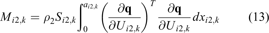
Ψ_{i 2, k} = [\begin{matrix} 0_{4 \times 1} \\ 1 - 3 x_{i 2, k}^{2} / a_{i 2, k}^{2} + 2 x_{i 2, k}^{3} / a_{i 2, k}^{3} \\ x_{i 2, k} - 2 x_{i 2, j}^{2} / a_{i 2, k} + x_{i 2, k}^{3} / a_{i 2, k}^{2} \\ 3 x_{i 2, k}^{2} / a_{i 2, k}^{2} - 2 x_{i 2, k}^{3} / a_{i 2, k}^{3} \\ - x_{i 2, k}^{2} / a_{i 2, k} + x_{i 2, k}^{3} / a_{i 2, k}^{2} \end{matrix}]

The element mass matrix is a $8 \times 8$ matrix and can be expressed as

M_{i 2, k} = ρ_{2} S_{i 2, k} \int_{0}^{a_{i 2, k}} {(\frac{\partial q}{\partial U_{i 2, k}})}^{T} \frac{\partial q}{\partial U_{i 2, k}} d x_{i 2, k}

The elastic potential energy is described as

V_{i 2, k} = \frac{1}{2} U_{i 2, k}^{T} K_{i 2, k} U_{i 2, k}

where

K_{i 2, k} = [\begin{matrix} 0_{4 \times 4} & 0_{4 \times 4} \\ 0_{4 \times 4} & K_{i 2, k,22} \end{matrix}]

$K_{i 2, k,22}$ has a similar form as $K_{i 1, k,22}$ .

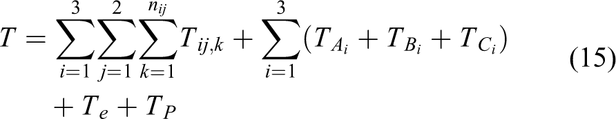
Therefore, the total kinetic energy of the V3 manipulator is the summation of the kinetic energies of all elements on the six links, the kinetic energies of the nine joints $T_{A_{i}}$ , $T_{B_{i}}$ , and $T_{C_{i}}$ , and the kinetic energies of the end-effector T_e and the payload T_p , which is given as follows

\begin{array}{l} T = \sum_{i = 1}^{3} \sum_{j = 1}^{2} \sum_{k = 1}^{n_{i j}} T_{i j, k} + \sum_{i = 1}^{3} (T_{A_{i}} + T_{B_{i}} + T_{C_{i}}) \\ + T_{e} + T_{P} \end{array}

where

T_{A_{i}} = \frac{1}{2} J_{A_{i}} {\dot{θ}}_{i}^{2}

T_{B_{i}} = \frac{1}{2} m_{B_{i}} {\dot{p}}_{B_{i}}^{T} {\dot{p}}_{B_{i}} + \frac{1}{2} J_{B_{i}} {({\dot{θ}}_{i} + {\dot{v}}_{i 1, e} + {\dot{γ}}_{i})}^{2}

T_{C_{i}} = \frac{1}{2} m_{C_{i}} {\dot{q}}_{C_{i}}^{T} {\dot{q}}_{C_{i}} + \frac{1}{2} J_{C_{i}} {({\dot{θ}}_{i} + {\dot{v}}_{i 1, e} + {\dot{γ}}_{i} + {\dot{v}}_{i 2, e})}^{2}

T_{e} = \frac{1}{2} m_{e} {\dot{q}}_{C_{1}}^{T} {\dot{q}}_{C_{1}} + \frac{1}{2} J_{e} {\dot{ϕ}}^{2}

T_{p} = \frac{1}{2} m_{p} {\dot{q}}_{C_{1}}^{T} {\dot{q}}_{C_{1}} + \frac{1}{2} J_{p} {\dot{ϕ}}^{2}

$m_{B_{i}}$ and $m_{C_{i}}$ are masses of joints, and $J_{A_{i}}$ , $J_{B_{i}}$ , and $J_{C_{i}}$ are moments of inertia of joints, m_e and J_e are mass and moment of inertia of the end-effector, m_p and J_p are mass and moment of inertia of the payload, respectively. $ϕ$ is the function of the coordinates of C_i .

Since only links are considered as flexible bodies, the total potential energy is the summation of all potential energies of all links

V = \sum_{i = 1}^{3} \sum_{j = 1}^{2} \sum_{k = 1}^{n_{i j}} V_{i j, k}

Boundary and constraint conditions

In this system model, the head of each link is clamped on the rotation axis of the joint, so that all links are fixed head beams. The flexural displaces and slopes of node 1 of each link are zeros

u_{i j,1} = 0, v_{i j,1} = 0, i = 1, 2, 3, j = 1, 2

Thus, the vector of generalized coordinate can be described by

r = {[\begin{matrix} θ_{1} & θ_{2} & θ_{3} & γ_{1} & γ_{2} & γ_{3} & R_{1}^{T} & R_{2}^{T} & R_{3}^{T} \end{matrix}]}^{T}

where

\begin{array}{l} R_{i} = [\begin{matrix} u_{i 1, 2} & v_{i 1, 2} & \dots & u_{i 1, n_{i 1}} & v_{i 1, n_{i 1}} & u_{i 1, e} & v_{i 1, e} \end{matrix} \\ {\begin{array}{l} u_{i 2, 2} & v_{i 2, 2} & \dots & u_{i 2, n_{i 2}} & v_{i 2, n_{i 2}} & u_{i 2, e} & v_{i 2, e} \end{array}]}^{T} \end{array}

are flexural displacements of the links. By using the generalized coordinate vector, the kinetic energy and potential energy in (15) and (16) can be summarized as

T = \frac{1}{2} {\dot{r}}^{T} M \dot{r}

V = \frac{1}{2} r^{T} K r

where M and K are the total mass matrix and the total stiffness matrix, obtained from those individual mass matrix and stiffness matrix, respectively.

Liao et al.¹⁸ have implemented an optimal kinematic design for the V3 robot manipulator, which presents the improved lengths of links. Here, the set of parameters will be applied to define the lengths in this study. In the end-effector, the length $b_{2} = 0$ , which means the bar $H_{3} H_{4}$ is vanished. The upper two subchains, thus, compose a five-bar mechanism. It is also regarded as a positioning device of the V3 manipulator. The orientation is controlled by the first subchain. The constraint conditions according to the loop-closure equations can be described as

H (r) = [\begin{matrix} {(x_{1} - x_{3})}^{2} + {(y_{1} - y_{3})}^{2} - b_{1}^{2} \\ x_{2} - x_{3} \\ y_{2} - y_{3} \end{matrix}] = 0

Dynamic equation

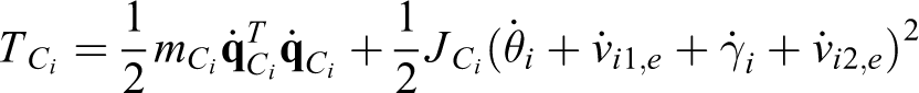
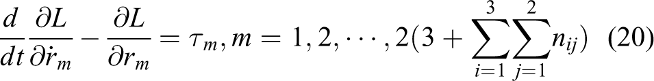
Lagrange multiplier $λ$ is employed to handle $L = T - V - H^{T} (r) λ$ The dynamic equation is thus obtained as

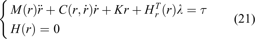
\frac{d}{d t} \frac{\partial L}{\partial {\dot{r}}_{m}} - \frac{\partial L}{\partial r_{m}} = τ_{m}, m = 1, 2, \dots,2 (3 + \sum_{i = 1}^{3} \sum_{j = 1}^{2} n_{i j})

where $τ_{m}$ is the generalized torque (force) corresponding to the mth generalized coordinate variable. By mathematic operation, the dynamic equation becomes

\{\begin{array}{l} M (r) \ddot{r} + C (r, \dot{r}) \dot{r} + K r + H_{r}^{T} (r) λ = τ \\ H (r) = 0 \end{array}

where M and K are mass and stiffness matrices, respectively, C is the Coriolis matrix, which can be calculated from M,³²

C_{i j} (r, \dot{r}) = \frac{1}{2} \sum_{k = 1}^{n} (\frac{\partial M_{i j}}{\partial r_{k}} + \frac{\partial M_{i k}}{\partial r_{j}} - \frac{\partial M_{k j}}{\partial r_{i}}) {\dot{r}}_{k}

H_r is the Jacobian matrix of constraint conditions (19) respecting to the general coordinate and satisfying $H_{r} \dot{r} = 0$ . Since no nonconservative force applied on r_m , $m = 4, \dots,2 (3 + \sum_{i = 1}^{3} \sum_{j = 1}^{2} n_{i j})$ , the generalized torques are characterized by the vector

τ = {[\begin{array}{l} τ_{1} & τ_{2} & τ_{3} & 0 & \dots & 0 \end{array}]}^{T}

where $τ_{i}$ , $i = 1, 2, 3$ are the actuated torques of each subchain.

Differential–algebraic equations are difficult to solve directly. The equation set (21) is one case. By differentiating (19) twice, the displacement constraints are transformed to the velocity and acceleration constrains. Therefore, the equation set (21) can be rewritten as

[\begin{matrix} M (r) & H_{r}^{T} \\ H_{r} & 0 \end{matrix}] [\begin{matrix} \ddot{r} \\ λ \end{matrix}] = [\begin{matrix} τ - C (r, \dot{r}) \dot{r} - K r \\ - {\dot{H}}_{r} \dot{r} \end{matrix}]

Then, we obtain ordinary differential equations, which can be solved by Runge–Kutta method.

Integrated design problem formulation

Controller

For high-speed robot control, many efficient control strategies have been introduced. Theoretically, any reasonable control strategy can be used to implement the integrated design. However, to check the performance of this integrated design initially, we expect to utilize a fundamental but effective control strategy. The PD controller is one of the most frequently used controllers in the industry.¹² It is fortunate if a simple controller can realize a good effect. It is undeniable that other advanced controllers, such as active disturbance rejection adaptive controller,³³ variable parameters controller, and fuzzy logic controller, can achieve better results, especially in the electronic industry. For the pick-and-place operations with variable payloads, these control methodologies must be more effective. To further improve the performance of the V3 robot system, these advanced controllers must be investigated for the integrated structure and control design in the future. But in this early study, PD controller is applied first. During the control process, it is ssvery difficult to measure the flexure on line. The actuated angle $θ_{i}$ at joint A_i ( $i = 1, 2, 3$ ) are the quantities that can be easily measured in real time. The velocity can be achieved by difference technique. By the PD control law, the input torque can be calculated as follows

τ_{i} = K_{p i} e_{i} + K_{d i} {\dot{e}}_{i}

where $e_{i} = θ_{d i} - θ_{i}$ , ${\dot{e}}_{i} = {\dot{θ}}_{d i} - {\dot{θ}}_{i}$ , and $θ_{d i}$ and ${\dot{θ}}_{d i}$ are the desired joint position and the desired joint angular velocity, respectively. $K_{p i}$ and $K_{d i}$ are nonnegative control parameters to be determined. Thus, a closed-loop control system, which contains structural and control parameters, is obtained by combining (23) and (24). Figure 4 shows the control process of the manipulator.

Figure 4.

The control block diagram.

Performance indices

The demanding requirements for automatic equipments can be translated into instantaneous and steady-state performances in a direct way. There are several performance indices, which can be chosen to characterize a system.

Settling time. It shows how long a system response enters a steady state. And it reflects the response speed of a system.

Steady-state error. This performance index is applied to characterize the system accuracy in steady-state.

The maximum value of the tracking error. This maximum value $e_{t m}$ is a performance index symbolizing the accuracy of the motion trajectory.

The ending value of the tracking error. The less is the ending value $e_{t e}$ , the closer to the steady-state is the system. It is a performance index reflecting accuracies of the picking or placing position and orientation.

The maximum value of the elastic potential energy. This performance index (V_m ) reflects the maximum elastic deformation of the whole robot mechanism in the trajectory. Simultaneously, the elastic deformation can be used to characterize the amplitude of vibration from a profile.

For a high-speed pick-and-place task, the object has usually been picked or placed before the system reaches its steady state. And the motion time is usually given in advance. Consequently, steady-state error and setting time are the common performance indices.^15,34,35 They will not be utilized in this article. The accuracy of the operation position, which is at the end of the trajectory, is most significant in a pick-and-place operation. Bounding values may help to complete the picking or placing task with high accuracy. The maximum value of the tracking error is secondary, while the ending value of the tracking error must be taken into account seriously. The tracking error originates from the actuated module, joint clearance, flexible link, and so on. During high-speed motion, if the tracking error is limited, the flexibility effects of the links will be reduced, and the vibration will also be attenuated. The flexibility effect generates elastic deformation, which comes with vibration. The extreme elastic deformation may make link bent largely, even broken off. Since the elastic potential energy reflects the elastic deformation, limiting the maximum value of elastic potential energy in the motion can constrain the elastic deformations and vibrations of the links.

Since the V3 robot manipulator has two translations and one rotation, the tracking errors can be determined as the tracking translation error $e_{t_{t}} = \sqrt{{(x_{d} - x)}^{2} - {(y_{d} - y)}^{2}}$ and the tracking rotation error $e_{t_{r}} = | ϕ_{d} - ϕ |$ , where x_d , y_d , and $ϕ_{d}$ are the desired position and orientation of the end-effector, respectively.

Design variables

Both structural and control parameters are optimized simultaneously in integrated design. In the dynamic model, $S_{i j, k}$ , $a_{i j, k}$ are structural parameters under determination. Therefore, the indeterminant structural parameters are $S_{i j, k}$ and $a_{i j, k}$ . Take $S = [S_{11, 1}, \dots, S_{11, n_{11}}, S_{12, 1}, \dots, S_{12, n_{12}}, \dots]^{T}$ and $A = [a_{11, 1}, \dots, a_{11, n_{11}}, a_{12, 1}, \dots, a_{12, n_{12}}, \dots]^{T}$ as the vector of cross-sectional area and length parameters, respectively. Take $K_{p} = [K_{p 1}, K_{p 2}, K_{p 3}]^{T}$ and $K_{d} = [K_{d 1}, K_{d 2}, K_{d 3}]^{T}$ as the vectors of control parameters. In summary, the set of design variables $P$ are the collection of both control parameters and structural parameters as follows

P = [K_{p}^{T}, K_{d}^{T}, S^{T}, A^{T}]^{T}

Problem formulation

Efficiency is a crucial target in a pick-and-place operation. Hence, the cycle time for each task should be as short as possible. In this study, the ending values of the tracking errors $e_{t_{t} e}$ and $e_{t_{r} e}$ , reflecting the achievement, should be minimized to complete the picking or placing task with high accuracy. The maximum values of the tracking errors $e_{t_{t} m}$ and $e_{t_{r} m}$ should be limited to satisfy the motion trajectory. Meanwhile, to decrease the effect of vibration, an effective and efficient way is to minimize the maximum value of elastic potential energy V_m . Furthermore, the actuated torque $τ$ also should be limited since actuated saturation exists for each actuator. Apparently, the above-mentioned problem can be formulated as a multiobjective optimization problem. Considering its complexity, some of the objective functions can be treated as constraints. In practice, it is difficult to given an appropriate range for the elastic potential energy, while the accuracy can be ensured as long as the error is limited in a small range. Those constraints are employed to ensure operational effectiveness. Then, according to the analyses above, the integrated design problem can be formulated as follows.

Problem 1. Integrated design problem based on elastic potential energy.

Find a set of optimal design parameters $P$ to

\begin{array}{l} min_{P} V_{m} \\ Subject to e_{t_{t} e} ⩽ e_{1}, e_{t_{r} e} ⩽ e_{2} \\ e_{t_{t} m} ⩽ e_{3}, e_{t_{r} m} ⩽ e_{4} \\ τ_{i} ⩽ τ_{max}, i = 1, 2, 3 \end{array}

where e_n , $n = 1, \dots,4$ , are the prespecified tracking errors bounds and $τ_{max}$ is considered as the actuated torque limit.

This formulation is a general framework of the integrated design for pick-and-place operations. For a defined manipulator with a trajectory, these constraints will be determined.

Simulation and discussion

Before the simulation, some symbols of lengths, materials, masses, and moments of inertia should be set specified values.

The lengths of links are obtained from our previous study,¹⁸ the lengths of actuated links $l_{i 1} = 0.306 m$ ( $i = 1, 2, 3$ ), the lengths of passive links $l_{i 2} = 0.532 m$ , $b_{1} = 0.069 m$ , and $b_{2} = 0 m$ .

In this case, we first consider simple discrete model, while focus on the performance improvement of the manipulator with variable cross-sectional links. The actuated links $i 1$ ( $A_{i} B_{i}$ ) are discretized into two elements averagely ( $a_{i 1, k} = l_{i 1} / 2$ ) and for passive links $i 2$ ( $B_{i} C_{i}$ ), $k = 3$ ( $a_{i 2, k} = l_{i 2} / 3$ ). Suppose the links are cylinders, the cross-sectional areas are, thus, the functions of the radii. In the implementation, the structural parameters are only the radii (R ₁ and R ₂ for links $i 1$ , r ₁, r ₂, and r ₃ for links $i 2$ ). Therefore, $S = [R_{1}, R_{2}, r_{1}, r_{2}, r_{3}]^{T}$ .

In real-world, the torque of any electric motor cannot be unlimitedly increased. Usually, an actuated system in an industrial equipment is composed of one motor and one gearbox. In this simulation, the limitation of an actuated system is supposed to be $τ_{max} = 120 N \cdot m$ .

Aluminium alloy is chosen as the material of actuated links. Its density is $2.7 \times 10^{3} kg/m^{3}$ and Young’s modulus is $71 GPa$ . Carbon fiber is chosen as the material of the passive links. Its density is $1.8 \times 10^{3} {kg/m}^{3}$ and Young’s modulus is $150 GPa$ .

$J_{A_{i}} = 0.2 kg \cdot m^{2}$ , $J_{B_{i}} = 0.005 kg \cdot m^{2}$ , $m_{B_{i}} = 0.5 kg$ , $J_{C_{i}} = 0.005 kg \cdot m^{2}$ , $m_{C_{i}} = 0.5 kg$ , $i = 1, 2, 3$ , $J_{e} + J_{p} = 0.005 kg \cdot m^{2}$ , and $m_{e} = m_{p} = 0.5 kg$ . Note: The payload at the end-effector is not usually fixed for pick-and-place applications, especially in the electronic industry. The manipulator may pick up many different kinds of electronic components on one assembly line, such as printed circuit board, chipset, and so on, whose weights are not bigger than 0.5 kg. The maximum payload case in this integrated structure and control design is considered as the extreme case. Small load changing does not affect the performance very much. When the performance of the extreme case is improved, the performance of the unload case also becomes better. Thus, we can only focus on the extreme case in this optimal design.

In general, a linear trajectory is usually selected in a pick-and-place operation. In this case, the end-effector will be moved from the position $(0.75, - 0.15)$ to the desired position $(0.75, 0.15)$ (units: m) and rotated from $- 3 π / 4$ to $- π / 2$ (units: rad). And the triangular velocity planning with no singularities is chosen, which is fulfilled in $0.14$ s. The sampling period is fixed to be $200$ $µ$ s. Thus, the desired trajectories can be presented as follows

When $t \leq 0.07$ s

x = 0.75

y = - 0.15 + 0.5 \times \frac{(0.15 - (- 0.15))}{{(0.14 / 2)}^{2}} t^{2}

ϕ = - 3 π / 4 + 0.5 \times \frac{((- π / 2) - (- 3 π / 4))}{{(0.14 / 2)}^{2}} t^{2}

When 0.07 s $< t \leq$ 0.14 s

x = 0.75

y = 0.15 - 0.5 \times \frac{(0.15 - (- 0.15))}{{(0.14 / 2)}^{2}} {(0.14 - t)}^{2}

ϕ = - π / 2 - 0.5 \times \frac{((- π / 2) - (- 3 π / 4))}{{(0.14 / 2)}^{2}} {(0.14 - t)}^{2}

Due to the rotational symmetry of the V3 manipulator architecture, its characteristics are studied only in radial direction in workspace.¹⁸ For any configuration, there must be a configuration with the same performance at another radius. They are symmetrical configurations. Therefore, any selected trajectory has infinite symmetrical trajectories, which all can satisfy these required indices. To measure the tracking errors, the coordinates of the end-effector can be calculated by the flexible kinematics. The choices of the control parameters are the expectations of the errors of the positions and the velocities. First, beginning from a regular example, $K_{p i} = 1.2 \times 10^{5}$ , $K_{d i} = 800$ , $R_{j} = 0.02 m$ , $r_{i} = 0.01 m$ , $i = 1, 2, 3$ , $j = 1, 2$ , the variations of the elastic potential energy, and the errors and the actuated torques in the operation can be analyzed. Moreover, the ordinary differential equations are calculated by the MATLAB ode45 solver. The tracking errors depend on the position coordinate of the end node of each subchain. The translation error is described by the desired position and the point C ₁. The orientation of the end-effector can be calculated by coordinates of the points C ₁ and C ₂ (or C ₃). These points’ coordinates are determined by the actuated and the passive angles, the flexural displaces, and the slopes at the ends of $l_{i 1}$ and $l_{i 2}$ , $i = 1, 2, 3$ , which can be described as equation (9). Figures 5 and 6 show the tracking errors in X-direction, Y-direction, and orientation, respectively. In accelerating stage, the translation error increases rapidly at beginning, while at beginning of the decelerating stage, the error becomes negative quickly, since deceleration can be considered as acceleration in the opposite direction. The peak value of $e_{t_{t}}$ , which is more than $2.5 mm$ , appears at about $0.088 s$ . At the end of the deceleration, the translation error reduces, but the value is also more than $1 mm$ . The primary cause of the irregular change of the orientation error is that the errors of the point C ₁ and C ₂ (or C ₃) cannot change in the same trend. However, the peak value of the orientation error $e_{t_{r}}$ is less than $5 \times 10^{- 3} rad$ ( $5 \times 10^{- 3} rad$ $\approx$ $0.29 deg$ ). The elastic energy depends on the flexural displaces and slopes of all the nodes. Simultaneously, it reflects the vibration effect from another perspective. Figure 7 shows the elastic potential energy response in this operation. The peak value $0.27 J$ appears in the changeover period between acceleration and deceleration. And the vibration is more obvious in the deceleration. Figure 8 shows the actuated torques responses of the system. The $τ_{2}$ and $τ_{3}$ reach the boundary in this operation.[Please approve the edits made in table citations.]

Figure 5.

The translation tracking errors with a set of regular parameters: (a) in X-direction and (b) in Y-direction.

Figure 6.

The orientation tracking errors with a set of regular parameters.

Figure 7.

The elastic potential energy response with a set of regular parameters.

Figure 8.

The actuated torque responses with a set of regular parameters.

The choices of the prespecified tracking errors bounds depend on the results of the simulation example and the requirements of pick-and-place operations.

The translation tracking errors bounds: $e_{1} = 0.001 m$ and $e_{3} = 0.003 m$ .

The rotation tracking errors bounds: $e_{2} = 5 \times 10^{- 4} rad$ and $e_{4} = 5 \times 10^{- 3} rad$ .

These ending values of the tracking errors can satisfy the most requirements of pick-and-place operations.

In simulation, the integrated design problem is realized as follows.

Problem 2. Integrated design of V3 parallel manipulator based on elastic potential energy

Find a set of optimal design parameters $P = [K_{p 1}, K_{p 2},$ $K_{p 3}, K_{d 1}, K_{d 2}, K_{d 3}, R_{1}, R_{2}, r_{1}, r_{2}, r_{3}]^{T}$ to

\begin{array}{l} min_{P} V_{m} \\ Subject to e_{t_{t} e} ⩽ e_{1}, e_{t_{r} e} ⩽ e_{2} \\ e_{t_{t} m} ⩽ e_{3}, e_{t_{r} m} ⩽ e_{4} \\ | τ_{i} | ⩽ τ_{max}, i = 1, 2, 3 \\ K_{p 1}, K_{p 2}, K_{p 3} \in [10 \times 10^{5},1.5 \times 10^{5}] \\ K_{d 1}, K_{d 2}, K_{d 3} \in [500, 1000] \\ R_{1}, R_{2} \in [0.015 m,0.045 m] \\ r_{1}, r_{2}, r_{3} \in [0.005 m,0.015 m] \end{array}

This integrated design problem, by analyzing, is a nonlinear and nonconvex optimization problem. Thus, the genetic algorithm (GA) will be chosen to solve this optimization problem. To improve the computational efficiency, the GA toolbox and the parallel computing toolbox in MATLAB are utilized. The GA toolbox uses matrix functions to build a set of versatile routines for implementing a wide range of GA methods.³⁶ The parallel computing toolbox solves computationally and data-intensive problems using multicore processors, GPUs, and computer clusters.³⁷ Let consumers use the full processing power of multicore computers.

There are 11 parameters to be designed. If the optimum is searched directly, it is time-consuming. Hence the integrated design can be thus in two steps. It is assumed that the cross-sectional areas of the elements on links $i 1$ and $i 2$ ( $i = 1, 2, 3$ ) are united, respectively, in the first step, that is, $R_{1} = R_{2} : = R$ and $r_{1} = r_{2} = r_{3} : = r$ . It leads to eight independent design variables. For another purpose, it is used to consider the integrated design with the same shapes of the manipulator links. In the first step, the initial set is generated randomly and uniformly in the parameter intervals. Once a set satisfies all the constraints, it is regarded as an effective initial set and is applied to initialize the search. When the optimum is found in this step, it is served as the initial set for the second-step integrated design, which takes all 11 parameters as independent ones.

The initial and the optimal parameters generated by first-step integrated design are shown in Table 2. Comparing with the control parameters, the structural parameters change little. In the optimal design, $K_{p 3}$ is smallest in the $K_{p i}$ , $i = 1, 2, 3$ , but $K_{d 3}$ is biggest in the $K_{d i}$ . Figures 9 and 10 show the translation and orientation trajectories with the first-step initial and optimal parameters, respectively. There are small errors between the simulated controlled responses and the planned trajectories. In the accelerating stages of the initial and optimal design, the translation tracking errors increase rapidly at the beginning and the end, as shown in Figure 11. At the end of these operations, the translation errors achieve the peak values, $0.84 mm$ with the initial design and $0.99 mm$ with the optimal design. The $e_{t_{t}}$ of the optimal design is not obviously fluctuant. Figure 12 shows that the maximum value of the orientation tracking error of the initial design is $8.31 \times 10^{- 4} rad$ and the end value is $8.26 \times 10^{- 5} rad$ , and $e_{t_{r} m} = 1.23 \times 10^{- 3} rad$ and $e_{t_{r} e} = 3.98 \times 10^{- 4} rad$ , respectively, with the optimal design, which increase apparently. However, the elastic potential energy is effectively controlled by the first-step optimization, as shown in Figure 13. The maximum value of the elastic potential energy of the initial design is $0.0459 J$ , which also appears in the acceleration changeover period. In the optimal system, the V_m is $0.0184 J$ , which is lowered by $59.91 %$ . And at the end of the operation, the plot of the elastic potential energy becomes gentle. It implies the vibration is weakened. Figure 14 shows the actuated torque responses with optimal parameters. At the end of the accelerating and the decelerating stage, the $τ_{2}$ reaches the boundary. And the $τ_{3}$ reaches the boundary at the beginning of the decelerating stage. The convergence of the first-step integrated design process is shown in Figure 15.

Table 2.

The initial and optimal design generated by the first-step integrated design.

	$K_{p 1}$	$K_{p 2}$	$K_{p 3}$	$K_{d 1}$	$K_{d 2}$	$K_{d 3}$
Initial	$131336$	$118194$	$134676$	$682$	$601$	$876$
Optimal	$124854$	$120571$	$108102$	$812$	$750$	$915$
	R(mm)		r(mm)
Initial	$34.12$		$10.12$
Optimal	$34.66$		$10.83$

Figure 9.

The translation trajectories with the first-step initial and optimal parameters.

Figure 10.

The orientation trajectories with the first-step initial and optimal parameters.

Figure 11.

The translation tracking errors with the first-step initial and optimal parameters: (a) in X-direction and (b) in Y-direction.

Figure 12.

The orientation tracking errors with the first-step initial and optimal parameters.

Figure 13.

The elastic potential energy responses with the first-step initial and optimal parameters.

Figure 14.

The actuated torque responses with the first-step optimal parameters.

Figure 15.

The convergence of the first optimizing process.

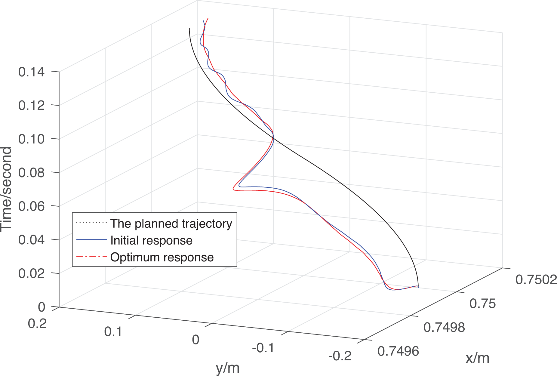
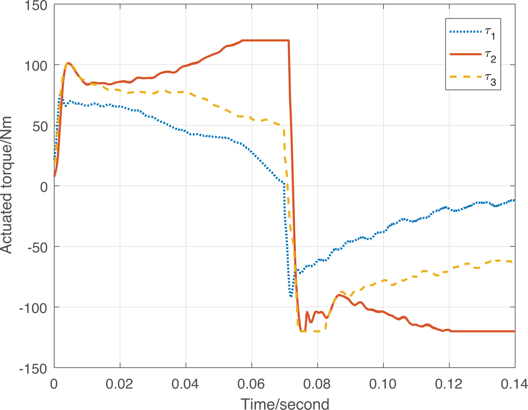
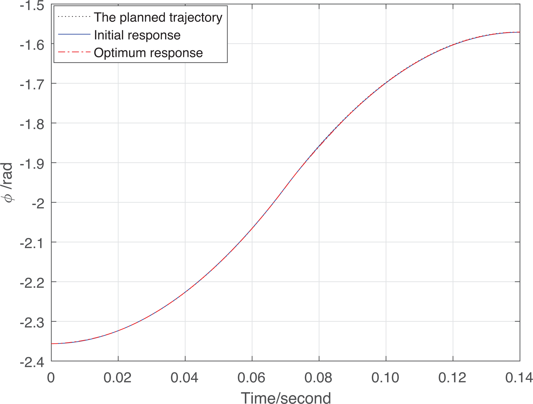
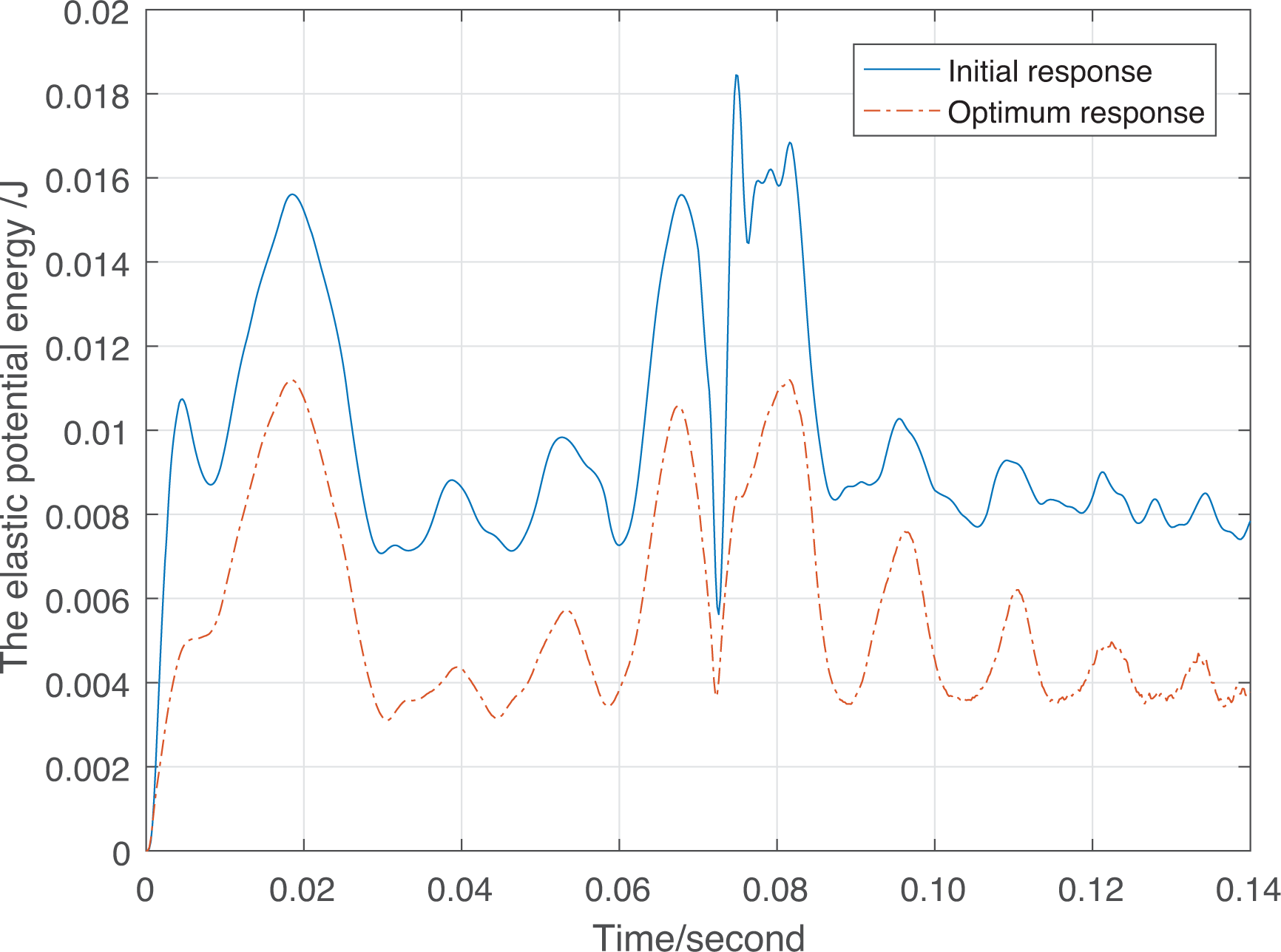
The second-step integrated design started from the results (the optimal parameters) of the first-step design. Table 3 shows the comparison of the initial and optimal parameters. $K_{p i}$ , $i = 1, 2, 3$ , and $K_{d j}$ , $j = 1, 2$ , increase in varying degrees. But $K_{d 3}$ reduce, which is the smallest in the optimal control parameters. For the structural parameters, the radii of the links change obviously. For the link $i 1$ , not only the radius of the first element but also the radius of the second element become greater. The radius of the first element is bigger than the second element’s, which increases about $26.92 %$ . The variation of the radius of the second element is less than $1 mm$ . For the link $i 2$ , the radius of the first element increases about $0.2 mm$ . The radii of the second and third elements reduce $0.18 mm$ and $0.9 mm$ , respectively. Figures 16 and 17 show the translation and orientation trajectories with the second-step initial and optimal parameters, respectively. The responses with the optimal parameters are better. From Figure 18, we can know that the variation trend of the translation tracking error of the optimal design is similar to the initial one. The maximum value of the optimal design also appears at the end of the operation, $e_{t_{t} m} = e_{t_{t} e} = 0.98 mm$ . In the translation tracking errors in X-direction, the optimum response is worse than the initial response after 0.08 s in a short time. It mainly causes by high deceleration. However, this local peak value is significantly smaller than the maximum value. This phenomenon can be accepted. The maximum values and the ending values of the tracking errors in X-direction and Y-direction are not beyond the constraints. The orientation tracking errors are shown in Figure 19. The peak value of the orientation tracking error of the optimal design is $2.11 \times 10^{- 3} rad$ , which does not reduce, and the end value is $1.40 \times 10^{- 5} rad$ . After the second-step integrated design, the elastic potential energy is lowered again, see Figure 20. The V_m of the optimal design is $0.0112 J$ . The vibration of the operation is controlled better. Figure 21 shows the actuated torque responses with the second-step optimal parameters. In the decelerating stage, the actuated torque responses gradually begin to oscillate obviously. The $τ_{1}$ response oscillates most at the end of this operation. The $τ_{2}$ also reaches the boundary at the end of the accelerating and the decelerating stage, and the $τ_{3}$ reaches the boundary at the beginning of the decelerating stage. Figure 22 shows the convergence of the second-step integrated design process.

Table 3.

The initial and optimal design generated by the second-step integrated design.

	$K_{p 1}$	$K_{p 2}$	$K_{p 3}$	$K_{d 1}$	$K_{d 2}$	$K_{d 3}$
Initial	$124854$	$120571$	$108102$	$812$	$750$	$915$
Optimal	$141436$	$129506$	$122940$	$840$	$834$	$560$
	R ₁(mm)	R ₂(mm)	r ₁(mm)	r ₂(mm)	r ₃(mm)
In	$34.66$	$34.66$	$10.83$	$10.83$	$10.83$
Op	$43.99$	$35.52$	$11.03$	$10.65$	$9.93$

Figure 16.

The translation trajectories with the second-step initial and optimal parameters.

Figure 17.

The orientation trajectories with the second-step initial and optimal parameters.

Figure 18.

The translation tracking errors with the second-step initial and optimal parameters: (a) in X-direction and (b) in Y-direction.

Figure 19.

The orientation tracking errors with the second-step initial and optimal parameters.

Figure 20.

The elastic potential energy responses with the second-step initial and optimal parameters.

Figure 21.

The actuated torque responses with the second-step optimal parameters.

Figure 22.

The convergence of the second optimizing process.

Comparison

In this section, the results of conventional design in which the structural parameters $P_{s} = [R_{1}, R_{2}, r_{1}, r_{2}, r_{3}]^{T}$ are optimized first and the control parameters $P_{c} = [K_{p 1}, K_{p 2}, K_{p 3}, K_{d 1}, K_{d 2}, K_{d 3}]^{T}$ second is shown to compare with the results of integrated design. The set of regular parameters in “Simulation and Discussion” is chosen as the initial parameters. The design problem is similar to Problem 2 but the design parameters are divided into two sets. In the first step, to optimize the structural parameters, the control parameters are fixed to the initial parameters. When the optimal structural parameters are obtained, they remain unchanged to optimize the control parameters in the second step.

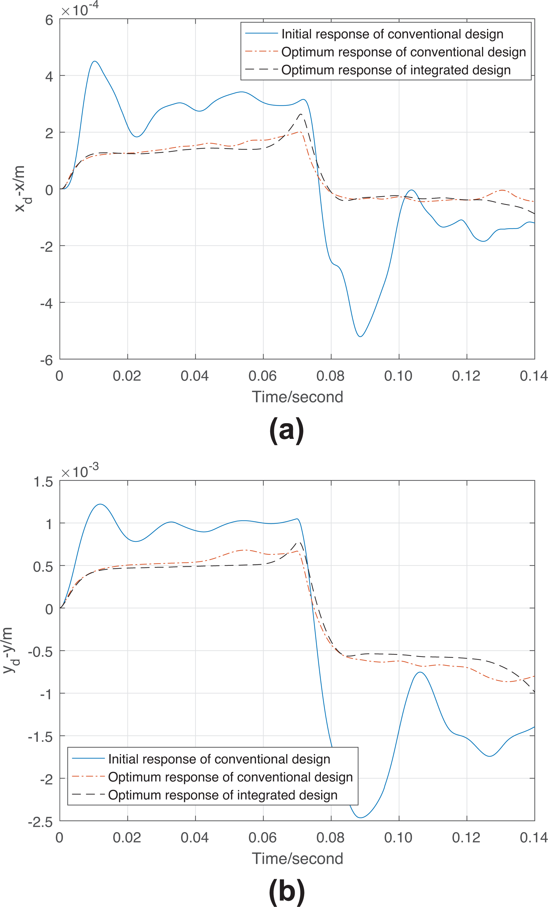
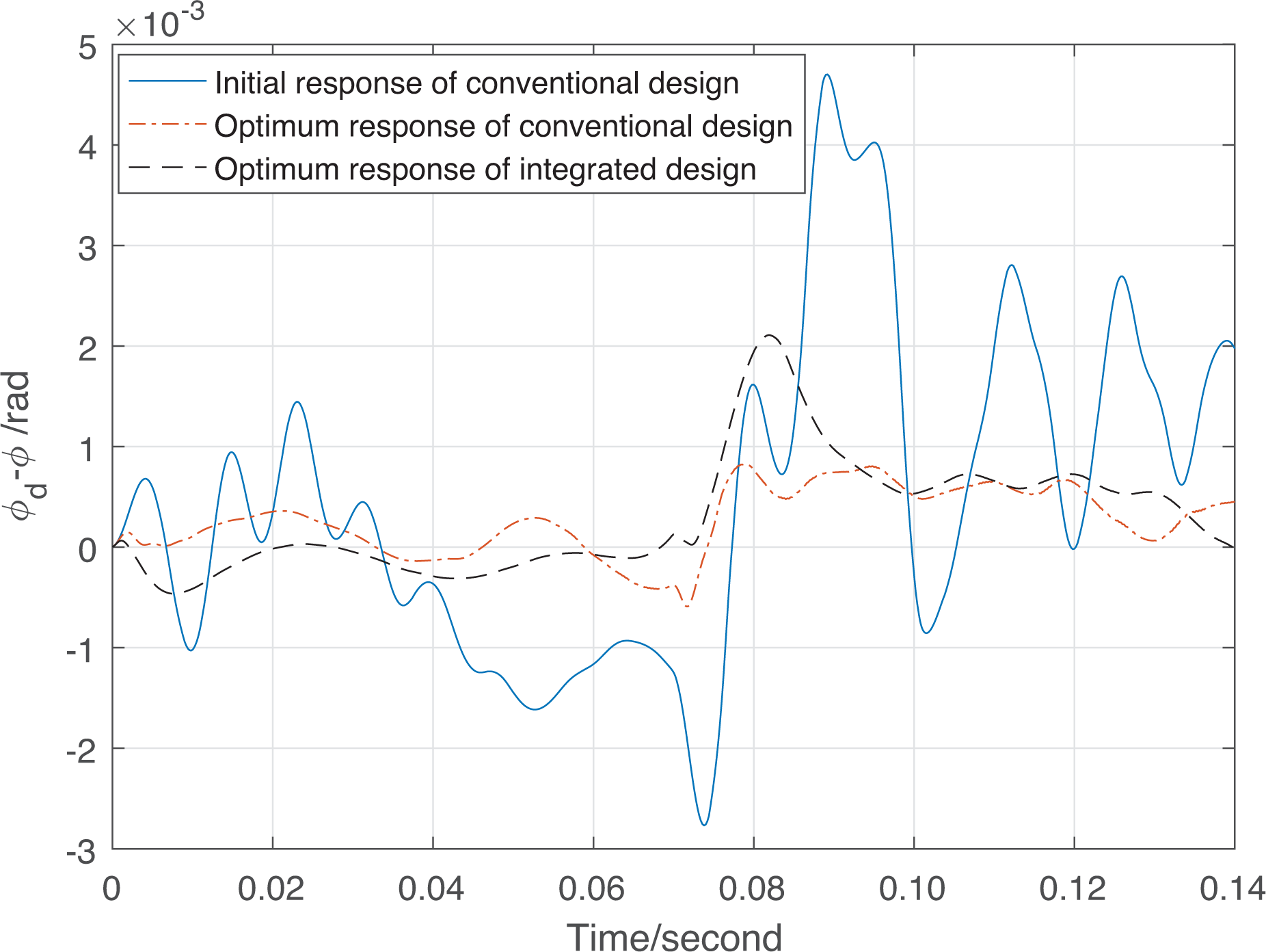
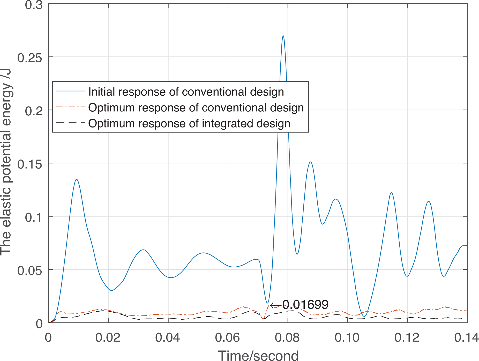
Table 4 shows the initial and optimal parameters. After the optimal design, the radii of the elements on the link $i 1$ become big. The radii of the first two elements on the link $i 2$ are nearly equal. The third element becomes small. For control parameters, $K_{p i}$ ( $i = 1, 2, 3$ ) decreases but $K_{d i}$ ( $i = 1, 2, 3$ ) increases. Figures 23 –26 show the tracking performances are not much better than the results of the integrated design, which all fulfill requests. However, the maximum value of the elastic potential energy after the conventional design is 0.01699 J, which is bigger than 1.5 times of V_m with the optimal parameters of the integrated design (see Figures 20 and 27). The actuated torque responses with the optimal parameters of conventional design fluctuate greatly in Figure 28. Figure 29 shows the convergence of the conventional design process. Thus, the integrated structure and control design method are more effective to improve the performance on elastic deformation.

Table 4.

The initial and optimal design generated by conventional design.

	$K_{p 1}$	$K_{p 2}$	$K_{p 3}$	$K_{d 1}$	$K_{d 2}$	$K_{d 3}$
Initial	$120000$	$120000$	$120000$	$800$	$800$	$800$
Optimal	$119577$	$116009$	$118713$	$822$	$823$	$808$
	R ₁(mm)	R ₂(mm)	r ₁(mm)	r ₂(mm)	r ₃(mm)
In	$20.00$	$20.00$	$10.00$	$10.00$	$10.00$
Op	$43.60$	$22.06$	$12.61$	$12.67$	$6.77$

Figure 23.

The translation trajectories with initial and optimal parameters of conventional design.

Figure 24.

The orientation trajectories with initial and optimal parameters of conventional design.

Figure 25.

The translation tracking errors with initial and optimal parameters of conventional design and optimal parameters of integrated design: (a) in X-direction and (b) in Y-direction.

Figure 26.

The orientation tracking errors with initial and optimal parameters of conventional design and optimal parameters of integrated design.

Figure 27.

The elastic potential energy responses with initial and optimal parameters of conventional design and optimal parameters of integrated design.

Figure 28.

The actuated torque responses with optimal parameters of conventional design.

Figure 29.

The convergence of the conventional design process.

Conclusion

A new integrated design framework based on elastic potential energy is presented in this article. And it is applied to design a coaxis planar parallel manipulator, V3. The FEM is utilized to derive the system dynamic model. A PD controller is employed in the closed-loop system to verify its effects. In this study, the vibration is suppressed via minimizing the maximum value of the elastic potential energy. For pick-and-place operation, the limitations of the actuated system, the ending, and maximum values of the tracking errors are also regarded as the major performance indices. Then, this integrated design problem is formulated as a nonlinear, multimodal optimization problem and the GA is applied to locate the global optimum. Last, the performance on elastic deformation for this manipulator system has been obviously improved by this integrated design method in the simulation. The vibration during the moving process can be controlled better. In further study, a prototype will be set up and the experiments will be carried out.

Footnotes

Declaration of conflicting interests

The author(s) declared no potential conflicts of interest with respect to the research, authorship, and/or publication of this article.

Funding

The author(s) disclosed receipt of the following financial support for the research, authorship, and/or publication of this article: This work was supported in part by Guangxi Natural Science Foundation under Grant 2019GXNSFBA245024, in part by Guangxi Science and Technology Program under Grant AD19245045, and in part by Innovation Driven Development Special Fund Project of Guangxi under Grant AA18118002-3.

ORCID iD

Bin Liao

References

Nabat

de la O Rodriguez

Company

, et al. Par4: very high speed parallel robot for pick-and-place. In 2005 IEEE/RSJ international conference on intelligent robots and systems, Edmonton, AB, Canada, 2–6 August 2005, pp. 553–558. IEEE.

Chen

, et al. Optimal design of a 2-DOF parallel manipulator with actuation redundancy considering kinematics and natural frequency. Robot Comput-Integr Manuf 2013; 29(1): 80–85.

Wang

Zhang

. Optimal design of a planar parallel 3-DOF nanopositioner with multi-objective. Mech Mach Theory 2017; 112: 61–83.

Jiang

Rui

Zhu

, et al. Optimal design of 6-DOF vibration isolation platform based on transfer matrix method for multibody systems. Acta Mechanica Sinica 2020; 37: 1–11.

Mohamed

Tokhi

. Command shaping techniques for vibration control of a flexible robot manipulator. Mechatronics 2004; 14(1): 69–90.

Hassan

Dubay

, et al. Active vibration control of a flexible one-link manipulator using a multivariable predictive controller. Mechatronics 2007; 17(6): 311–323.

Ouyang

Hong

. Vibration control of a flexible robotic manipulator in the presence of input deadzone. IEEE Trans Industr Inform 2016; 13(1): 48–59.

Hillsley

Yurkovich

. Vibration control of a two-link flexible robot arm. Dynamic Control 1993; 3(3): 261–280.

Karagülle

Malgaca

Dirilmis

, et al. Vibration control of a two-link flexible manipulator. J Vib Control 2017; 23(12): 2023–2034.

10.

Cao

Liu

. Boundary vibration control for a two-link rigid–flexible manipulator with quantized input. J Vib Control 2019; 25(23–24): 2935–2945.

11.

Maghami

Joshi

Lim

. Integrated controls-structures design: a practical design tool for modern spacecraft. In 1991 American control conference, Boston, MA, USA, 26–28 June 1991, pp. 1465–1473. IEEE.

12.

Zhang

, et al. Integrated design and PD control of high-speed closed-loop mechanisms. J Dyn Syst, Meas Control 2002; 124(4): 522–528.

13.

Rieber

Taylor

. Integrated control system and mechanical design of a compliant two-axes mechanism. Mechatronics 2004; 14(9): 1069–1087.

14.

Kim

Chung

. A systematic approach to design high-performance feed drive systems. Int J Mach Tools Manuf 2005; 45(12–13): 1421–1435.

15.

Lou

Zhang

Huang

, et al. Integrated structure and control design for a flexible planar manipulator. In International conference on intelligent robotics and applications, Aachen, Germany, 6–8 December, 2011, pp. 260–269. Springer.

16.

Lou

, et al. A parallel robotic mechanism having large workspace. China Patent 200910309684.2, 2009.

17.

Isaksson

. A family of planar parallel manipulators. In 2011 IEEE international conference on robotics and automation, Shanghai, China, 9–13 May, 2011, pp. 2737–2744. IEEE.

18.

Liao

Lou

. Kinematics and optimal design of a novel 3-DOF parallel manipulator for pick-and-place applications. Int J Mech Automat 2013; 3(3): 181–190.

19.

Liao

Kuang

Lou

, et al. Efficiency based integrated design of the V3 parallel manipulator for pick-and-place applications. In 2017 IEEE international conference on cybernetics and intelligent systems (CIS) and IEEE conference on robotics, automation and mechatronics (RAM), Ningbo, China, 19–21 November, 2017, pp. 213–218. IEEE.

20.

Liang

Song

Sun

, et al. Rigid-flexible coupling dynamic modeling and investigation of a redundantly actuated parallel manipulator with multiple actuation modes. J Sound Vib 2017; 403: 129–151.

21.

Zhang

. Analysis on rigid-elastic coupling characteristics of planar 3-RRR flexible parallel mechanisms. In International conference on intelligent robotics and applications, Wuhan, China, 16–18 August, 2017, pp. 394–404. Springer.

22.

Dwivedy

Eberhard

. Dynamic analysis of flexible manipulators, a literature review. Mech Mach Theory 2006; 41(7): 749–777.

23.

Green

Sasiadek

. Dynamics and trajectory tracking control of a two-link robot manipulator. J Vib Control 2004; 10(10): 1415–1440.

24.

Celentano

Coppola

. A computationally efficient method for modeling flexible robots based on the assumed modes method. Appl Math Comput 2011; 218(8): 4483–4493.

25.

Zhang

Mills

Cleghorn

, et al. Dynamic model and input shaping control of a flexible link parallel manipulator considering the exact boundary conditions. Robotica 2015; 33(6): 1201–1230.

26.

Gao

Zhou

, et al. Neural network control of a two-link flexible robotic manipulator using assumed mode method. IEEE Trans Ind Informat 2018; 15(2): 755–765.

27.

Piras

Cleghorn

Mills

. Dynamic finite-element analysis of a planar high-speed, high-precision parallel manipulator with flexible links. Mech Mach theory 2005; 40(7): 849–862.

28.

Dubay

Hassan

, et al. Finite element based model predictive control for active vibration suppression of a one-link flexible manipulator. ISA Trans 2014; 53(5): 1609–1619.

29.

Salerno

Zhang

Menciassi

, et al. A novel 4-DOF origami grasper with an SMA-actuation system for minimally invasive surgery. IEEE Trans Robot 2016; 32(3): 484–498.

30.

Wang

, et al. Stiffness modeling approach for a 3-DOF parallel manipulator with consideration of nonlinear joint stiffness. Mech Mach Theory 2018; 123: 137–152.

31.

Theodore

Ghosal

. Comparison of the assumed modes and finite element models for flexible multilink manipulators. Int J Robot Res 1995; 14(2): 91–111.

32.

Murray

Shankar Sastry

. A mathematical introduction to robotic manipulation. Boca Raton, FL: CRC Press, 1994; 7.

33.

Yao

Deng

. Active disturbance rejection adaptive control of uncertain nonlinear systems: theory and application. Nonlinear Dyn 2017; 89(3): 1611–1624.

34.

Hasanien

. Design optimization of PID controller in automatic voltage regulator system using Taguchi combined genetic algorithm method. IEEE Syst J 2012; 7(4): 825–831.

35.

Zhao

Duan

Wen

, et al. Distributed finite-time tracking of multiple non-identical second-order nonlinear systems with settling time estimation. Automatica 2016; 64: 86–93.

36.

Chipperfield

Fleming

Fonseca

. Genetic algorithm tools for control systems engineering. In Proceedings of adaptive computing in engineering design and control, Vol. 128. Citeseer, 1994, p. 133.

37.

Mathworks. parallel computing toolbox. https://ww2.mathworks.cn/help/parallel-computing/index.html?s_tid=CRUX_lftnav

An integrated structure and control design of a coaxis planar parallel manipulator for pick-and-place applications based on elastic potential energy

Abstract

Keywords

Introduction

Dynamic modeling

Kinetic energy and potential energy

Boundary and constraint conditions

Dynamic equation

Integrated design problem formulation

Controller

Performance indices

Design variables

Problem formulation

Simulation and discussion

Comparison

Conclusion

Footnotes

Declaration of conflicting interests

Funding

ORCID iD

References