Sage Journals: Discover world-class research

Abstract

This article proposes a new algorithm for real-time path planning in dynamic environments based on space-discretized curve-shortening flows. The so-called curve-shortening flow method shares working principles with the well-established elastic bands method and overcomes some of its drawbacks concerning numerical robustness and parameterability. This is achieved by efficiently applying semi-implicit time integration for evolving the path and secondly by developing a methodology for setting the algorithm’s parameters based on physical quantities. Different short- and long-term validation scenarios are performed with three interlinked instances of the curve-shortening flow method each running on an individual industrial control and driving a real or a simulated unmanned aerial vehicle.

Keywords

Path planning dynamic environment real-time unmanned aerial vehicle spatial path curve-shortening flow method elastic bands method

Introduction

Current developments in production engineering are driven by the demand for a high degree of individualization of consumer products. The accompanying variation in the sequence of the individual production steps and the demand-dependent occupancy of available processing machines requires intralogistics that are just as flexible. For transportation of small parts, the usage of unmanned aerial vehicles (UAVs) is currently widely studied. In contrast to fixed ground- and line-bound transportation devices (e.g. automated guided vehicles or conveyer belts), UAVs provide the possibility to exploit the normally unused airspace within the manufacturing plants. However, tasks that are independently assigned to the UAVs and executed in parallel can create an environment with high risk of collision, in which the individual flight movements of the UAVs cannot be planned in advance.

This leads to a dynamic and time-variant path-planning problem that can only be solved in real-time while considering the environment’s current state. With the so-called curve-shortening flow method (CFM), a new online path-planning algorithm capable of adjusting collision-free paths to a changing environment is presented.

Related work

The research field of mobile robotics provides numerous methods to solve for this type of path-planning problem that can also be applied to UAVs in general and especially to the here considered rotary wing UAVs like heli-, quad-, or multicopters which are able to hover and vertically start and land. These path-planning methods are typically classified into reactive, global, and mixed approaches.¹

Reactive path-planning methods such as virtual force field,² vector field histogram,^3
–5 nearness diagram,⁶ or dynamic window approach⁷ with origins in the potential field approach⁸ plan only short sections of the path based on local information without considering continuous connectivity to the goal. They primarily serve as collision-avoidance strategies and therefore are intricately linked with the robot’s motion control due to their ability to directly generate control signals in real time.⁹ At the same time, these methods are vulnerable to getting stuck in local minima or blockage and oscillation in close proximity to narrow passages^10,11 whereby a path to the goal cannot be guaranteed although it exists. Moreover, such reactive methods were developed for floor-bound mobile robots and are not applicable to three-dimensional path-planning problems in many cases.

Global path-planning methods are based on extensions of rapidly exploring random trees¹² (RRT) or probabilistic roadmaps¹³ (PRM) and represent a dynamic environment as a modifiable tree- or net-shaped connectivity graph of discrete and randomly picked collision-free points (samples) within the robot’s workspace. For instance, the RRT^x ¹⁴ and Real-time-RRT¹⁵ methods are capable of rewiring the arising tree structure in regards to dynamic obstacles at runtime. Dynamic roadmaps^16,17 or elastic roadmaps¹⁸ disable or relocate individual samples of a PRM net when occupied by dynamic obstacles.

As RRT-based methods pick random samples only during runtime and PRM-based methods need to execute an online-capable search algorithm such as Anytime A¹⁹ or D Lite,²⁰ the computation time to obtain a valid path is not predictable and makes them difficult to execute under hard real-time conditions. The large variation in execution times of typically more than 100 ms^1,21
–23 does also not guarantee a safe flight for dynamic UAVs using these methods.²⁴

Mixed path-planning methods like the elastic bands method²⁵ (EBM) or the elastic strips method²⁶ use local optimization by means of virtual forces in order to adapt an initially collision-free path to changes of the environment while simultaneously maintaining start and goal points as boundary conditions. The EBM matches the problem statement formulated in the introduction best because it can be efficiently reduced to a discrete description of a one-dimensional and deformable path in space with continuous curvature, global connectivity, and rapid response.

A significant weakness of the EBM lies in its insufficient numerical robustness due to updating the path using an explicit transition rule.²⁷ This insufficient numerical robustness leads to unpredictable oscillations or even instabilities when facing obstacles in close proximity and can only be compensated by a smaller step size and finer discretization of the path, which in turn worsens convergence and computational efficiency. While further developments of the EBM bypassed these stability issues using an optimization method,²⁷ the EBM’s original and computationally more efficient approach²⁵ to evolve the path with numerical integration was not continued by recent applications of the EBM in the field of mobile robotics,²⁸ service robotics,^29,30 or autonomous driving.³¹

These shortcomings are overcome by introducing the CFM. While maintaining the EBM’s working principle, the CFM provides numerically robust solvability under hard real-time conditions with cycle times of just a few milliseconds which are characteristic for industrial controls.

Curve-shortening flow method

Similar to the EBM, the CFM describes the path between a start p _s and a goal p _g as a sequence of n discrete and consecutive nodes p _i whose positions are continuously adjusted to the current state of the environment by virtual forces in order to keep them collision-free. Figure 1 illustrates the working principle of the CFM.

Figure 1.

Working principle of the curve-shortening flow method.

The obstacles’ geometries serve as the source of the repulsive forces f _i displacing the path, while retractive forces k _i which are proportional to the path’s curvature push the path into a state of minimum length. The path thereby converges toward an equilibrium representing a Pareto-optimal state between these two criteria. The path behavior (path dynamics and stationary displacement) is tuned via the scalar dynamics parameter T and the scalar repulsion parameter K.

Mathematical description

The evolution of a single node $p_{i} = {(x_{i}, y_{i}, z_{i})}^{T}$ during runtime can be mathematically expressed by the following generalized ordinary differential equation (ODE) which applies for all n nodes along the path.

T \cdot {\dot{p}}_{i} (t) = \underset{k_{i}}{\underset{︸}{(p_{i + 1} (t) - p_{i} (t)) + (p_{i - 1} (t) - p_{i} (t))}} + K \cdot f_{i} (p_{i} (t), h (t))

The linear description of the unamplified retractive force k _i depends on the path’s curvature and is built upon the sum of two vectors each pointing from p _i toward one of its adjacent nodes. This formulation traces back to a space-discretized approximation^32,33 of continuous curve flows^33,34 (which the CFM is named after) and implicitly ensures that k _i always points toward the inner side of the path’s curvature. The unamplified repulsive force f _i is typically derived from nonlinear distance calculations between p _i and a problem-specific representation of the obstacles’ geometries h . An exemplary model of the environment will be presented later in the “Modeling of the environment” section.

Each spatial component (row) of the generalized ODE in equation (1) can be written out in a linear form of state space system to represent the positions of the path’s n coupled nodes along this axis. Due to similarity only the subsystem for the y-axis is shown here.

T \cdot \underset{\dot{y}}{\underset{︸}{(\begin{matrix} {\dot{y}}_{1} \\ {\dot{y}}_{2} \\ {\dot{y}}_{3} \\ ⋮ \\ {\dot{y}}_{n - 2} \\ {\dot{y}}_{n - 1} \\ {\dot{y}}_{n} \end{matrix})}} = \underset{A}{\underset{︸}{(\begin{matrix} - 2 & 1 & 0 & \dots & 0 & 0 & 0 \\ 1 & - 2 & 1 & \dots & 0 & 0 & 0 \\ 0 & 1 & - 2 & \dots & 0 & 0 & 0 \\ ⋮ & ⋮ & ⋮ & ⋱ & ⋮ & ⋮ & ⋮ \\ 0 & 0 & 0 & \dots & - 2 & 1 & 0 \\ 0 & 0 & 0 & \dots & 1 & - 2 & 1 \\ 0 & 0 & 0 & \dots & 0 & 1 & - 2 \end{matrix})}} \cdot \underset{y}{\underset{︸}{(\begin{matrix} y_{1} \\ y_{2} \\ y_{3} \\ ⋮ \\ y_{n - 2} \\ y_{n - 1} \\ y_{n} \end{matrix})}} + \underset{b_{y}}{\underset{︸}{(\begin{matrix} y_{s} \\ 0 \\ 0 \\ ⋮ \\ 0 \\ 0 \\ y_{g} \end{matrix})}} + K \cdot \underset{f_{y}}{\underset{︸}{(\begin{matrix} f_{1, y} (p_{1}, h) \\ f_{2, y} (p_{2}, h) \\ f_{3, y} (p_{3}, h) \\ ⋮ \\ f_{n - 2, y} (p_{n - 2}, h) \\ f_{n - 1, y} (p_{n - 1}, h) \\ f_{n, y} (p_{n}, h) \end{matrix})}}

Because the vector f _y of the repulsive forces’ components along the y-axis depends on all components of p _i , f _y forms a generally nonlinear coupling between all spatial subsystems. The vector b _y contains the y-coordinates of the start $p_{s} = {(x_{s}, y_{s}, z_{s})}^{T}$ and the goal $p_{g} = {(x_{g}, y_{g}, z_{g})}^{T}$ . The state space representations for the x- and the z-directions can be expressed analogously.

Parameter influence

Figure 2 illustrates the qualitative effect of the scalar parameters T and K on the evolution and the stationary displacement of a planar path ( $p \in ℝ^{2}$ ) under influence of three individual point-obstacles.

Figure 2.

Influence of the repulsion parameter K and the dynamics parameter $T .$

The figure shows how a fivefold amplification of the repulsion parameter K at constant T (column-wise reading) increases the distance to the obstacles. However, an amplification of the dynamics parameter T by a factor of five at constant K (row-wise reading) causes a slower convergence of the path without affecting its stationary displacement (equilibrium state). The latter can be recognized by the higher density of the path evolution steps that were taken at equidistant time intervals for all four settings. The arrows indicate the repulsive (red) and retractive (green) force vectors acting on the initial and the stationary path.

Analytical parameterization

The dependencies of the path behavior from the parameters and the number of nodes will be quantitatively analyzed in order to enable a systematic procedure for setting the parameters K and T for a desired path behavior and a given number of nodes n.

Path dynamics

To be able to study the properties of the CFM and the influence of the parameters analytically, the linear and perpendicular line load with reach r ₀ shown in Figure 3 is used as a reference obstacle.

Figure 3.

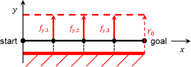
Using a linear line load as reference obstacle.

As here the vector of repulsive forces has an effect only in the y-direction, the analysis can be reduced to this component. With the above-described obstacle model $f_{i, y} = r_{0} - y_{i}$ , the linear state space representation from equation (2) can be expressed as follows*.

\underset{\dot{y}}{\underset{︸}{(\begin{matrix} {\dot{y}}_{1} \\ {\dot{y}}_{2} \\ {\dot{y}}_{3} \\ ⋮ \\ {\dot{y}}_{n - 2} \\ {\dot{y}}_{n - 1} \\ {\dot{y}}_{n} \end{matrix})}} = \underset{system matrix A^{*} = \frac{1}{T} \cdot (A - K \cdot I)}{\underset{︸}{(\begin{matrix} - \frac{2 + K}{T} & \frac{1}{T} & 0 & \dots & 0 & 0 & 0 \\ \frac{1}{T} & - \frac{2 + K}{T} & \frac{1}{T} & \dots & 0 & 0 & 0 \\ 0 & \frac{1}{T} & - \frac{2 + K}{T} & \dots & 0 & 0 & 0 \\ ⋮ & ⋮ & ⋮ & ⋱ & ⋮ & ⋮ & ⋮ \\ 0 & 0 & 0 & \dots & - \frac{2 + K}{T} & \frac{1}{T} & 0 \\ 0 & 0 & 0 & \dots & \frac{1}{T} & - \frac{2 + K}{T} & \frac{1}{T} \\ 0 & 0 & 0 & \dots & 0 & \frac{1}{T} & - \frac{2 + K}{T} \end{matrix})}} \cdot \underset{y}{\underset{︸}{(\begin{matrix} y_{1} \\ y_{2} \\ y_{3} \\ ⋮ \\ y_{n - 2} \\ y_{n - 1} \\ y_{n} \end{matrix})}} + \underset{\begin{matrix} input \\ vector \end{matrix}}{\underset{︸}{\frac{K}{T} \cdot (\begin{matrix} 1 \\ 1 \\ 1 \\ ⋮ \\ 1 \\ 1 \\ 1 \end{matrix})}} \cdot \underset{inp .}{\underset{︸}{r_{0}}}

Since the system matrix $A^{*}$ is of tridiagonal Toeplitz form, its n eigenvalues $λ_{i}$ can be analytically determined in dependency with K, T, and n.³⁵

λ_{i} = \frac{1}{T} \cdot (- 2 + 2 \cdot cos (\frac{π \cdot i}{n + 1}) - K)

With $K = 0$ , the system is unexcited and represents the resetting of an initially displaced path to a straight line in absence of obstacles (eigenbehavior).

Based on the theory of linear systems and control,³⁶ the following characteristics of the path can be derived from the resulting eigenvalues:

The path dynamics are stable due to the real component of all eigenvalues being negative at all times.

The path dynamics are not capable of self-oscillation as all eigenvalues are solely real-valued at all times.

The dynamics of every individual node can be regarded as a series of n PT₁-elements and thus every node shows low-pass behavior of nth order in its core.

In addition, the path’s inertia can be estimated on the basis of the largest eigenvalue $λ_{max} = λ_{1}$ , since $λ_{1}$ defines the slowest mode which dominates the system’s overall dynamics by partially acting on all n nodes’ positions (system states). In decoupled form, this mode describes a first-order lag element (PT₁) whose settling time $T_{max} = 3 / | λ_{max} |$ correlates with the average settling time $T_{\emptyset} = (1 / n) \cdot \sum_{i = 1}^{n} T_{95, i}$ of the coupled nodes. The settling time $T_{95, i}$ denotes the duration until the ith node has decayed by 95%. The matching between $T_{max}$ and $T_{\emptyset}$ was verified using simulation for several parameter settings as shown in Figure 4.

Figure 4.

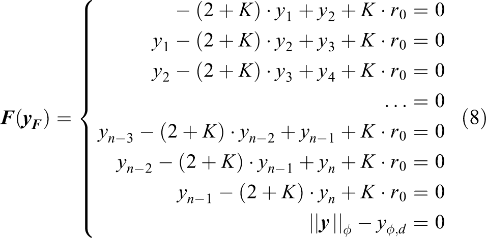
Correlation between $T_{max}$ (analytically calculated) and $T_{\emptyset}$ (simulated) for several parameter settings.

Figure 5 illustrates the evolution of the path under influence of a line load for the exemplary parameter setting highlighted in Figure 4.

Figure 5.

Evolution of the path excited by a line load obstacle.

Stationary displacement

Influenced by solely static obstacles, the nodes converge into a state of stationary displacement $p_{\infty}$ for $t \to \infty$ . This state can be used as a measure of the path’s safety distance. In analogy to the dynamic behavior, again the line load (see Figure 3) is used as a reference obstacle for the analysis of the y-component of the path.

For calculation of the stationary displacement of the nodes $y_{\infty}$ , equation (3) can be transformed into the linear system of equations (5) by zeroing its time derivatives $\dot{y} = 0$ . Since the solution $y_{\infty}$ is proportional to the reach r ₀, only the unified reach $r_{0} = 1 (m)$ is used in the following.

\underset{\begin{matrix} coefficent matrix \\ A - K \cdot I \end{matrix}}{\underset{︸}{(\begin{matrix} - 2 - K & 1 & 0 & \dots & 0 & 0 & 0 \\ 1 & - 2 - K & 1 & \dots & 0 & 0 & 0 \\ 0 & 1 & - 2 - K & \dots & 0 & 0 & 0 \\ ⋮ & ⋮ & ⋮ & ⋱ & ⋮ & ⋮ & ⋮ \\ 0 & 0 & 0 & \dots & - 2 - K & 1 & 0 \\ 0 & 0 & 0 & \dots & 1 & - 2 - K & 1 \\ 0 & 0 & 0 & \dots & 0 & 1 & - 2 - K \end{matrix})}} \cdot \underset{y_{\infty}}{\underset{︸}{(\begin{matrix} y_{1} \\ y_{2} \\ y_{3} \\ ⋮ \\ y_{n - 2} \\ y_{n - 1} \\ y_{n} \end{matrix})}} = - \underset{\begin{matrix} input \\ vector \end{matrix}}{\underset{︸}{K \cdot r_{0} \cdot (\begin{matrix} 1 \\ 1 \\ 1 \\ ⋮ \\ 1 \\ 1 \\ 1 \end{matrix})}}

Figure 6 shows the analytically calculated stationary paths for various repulsion parameters K and numbers of nodes n.

Figure 6.

Influence of K and n on the path’s stationary displacement.

It becomes clear that for $K \to \infty$ , the stationary displacement of the nodes $y_{\infty}$ is bounded by the reach r ₀ of the obstacles. Furthermore, an increase of n at constant K amplifies the displacement.

Calculation of the repulsion parameter

To achieve a desired stationary displacement, the corresponding value for K must be computed. To measure the overall displacement of the path with a single scalar indicator, the mean node displacement according to equation (6) is used.

{‖ y ‖}_{ϕ} = \frac{1}{n} \cdot \sum_{i = 1}^{n} | y_{i} |

By specifying the desired mean node displacement $y_{ϕ, d}$ with $0 < y_{ϕ, d} < r_{0}$ , the following boundary condition in equation (7) has to be fulfilled.

{‖ y ‖}_{ϕ} - y_{ϕ, d} = 0

In combination with equation (5), the nonlinear system of equations $F (y_{F}) = 0$ shown in equation (8) can be derived. Numerically solving for the vector of unknowns $y_{F} = {(y_{1}, y_{2}, y_{3}, \dots, y_{n}, K)}^{T} = {(y, K)}^{T}$ is accomplished using the Newton–Raphson method.³⁷

F (y_{F}) = {\begin{array}{r} - (2 + K) \cdot y_{1} + y_{2} + K \cdot r_{0} = 0 \\ y_{1} - (2 + K) \cdot y_{2} + y_{3} + K \cdot r_{0} = 0 \\ y_{2} - (2 + K) \cdot y_{3} + y_{4} + K \cdot r_{0} = 0 \\ \dots = 0 \\ y_{n - 3} - (2 + K) \cdot y_{n - 2} + y_{n - 1} + K \cdot r_{0} = 0 \\ y_{n - 2} - (2 + K) \cdot y_{n - 1} + y_{n} + K \cdot r_{0} = 0 \\ y_{n - 1} - (2 + K) \cdot y_{n} + K \cdot r_{0} = 0 \\ {‖ y ‖}_{ϕ} - y_{ϕ, d} = 0 \end{array}

Calculation of the dynamics parameter

The path dynamics are controlled via the dynamics parameter T. The earlier introduced average settling time $T_{\emptyset} \approx T_{max}$ is used as a measure for the inertia of the path. By specifying the desired settling time $T_{max, d}$ and considering the already known values for K and n in equation (4), the dynamics parameter T can be calculated according to equation (9).

\begin{matrix} T \end{matrix} (n, K, T_{max, d}) = \frac{1}{3} \cdot (2 - 2 \cdot cos (\frac{π}{n + 1}) + K) \cdot T_{max, d}

Time discretization

Solving the systems of ODEs in equation (2) is carried out using numerical time integration. The continuous time-derivative $\dot{p}$ is thereby approximated by a transition formula between two consecutive states of the path $p^{k} = p (t_{k})$ and $p^{k + 1} = p (t_{k + 1})$ with k indicating a time-discrete calculation step at time t_k with the constant step size $Δ t = t_{k + 1} - t_{k}$ .

The backward Euler method which has A-stability for linear time-invariant systems is used to allow for numerically robust time integration. To efficiently perform the integration steps, the (nonlinear) repulsive force f is evaluated explicitly (thus for the current state of the path p ^k ) and then fed component-wise into the ODEs as an input vector. This results in a semi-implicit execution of the backward Euler method which consequently loses its A-stability. Nevertheless, the method’s high degree of numerical damping still provides extraordinarily robust time integration.

Applying the discretization rules of the backward Euler method on equation (2) provides the following (semi-implicit) transition formula shown here for the y-component.

y^{k + 1} = y^{k} + \frac{Δ t}{T} \cdot (A \cdot y^{k + 1} + b_{y}^{} + K \cdot f_{y}^{k})

Rearranging equation (10) for the unknown $y^{k + 1}$ gives the linear system of equations (11) with the identity matrix I .

\underset{\begin{matrix} coefficent \\ matrix C \end{matrix}}{\underset{︸}{(I - \frac{Δ t}{T} \cdot A)}} \cdot \underset{\begin{matrix} sol . \\ vect . \end{matrix}}{\underset{︸}{y^{k + 1}}} = \underset{input vector r_{y}}{\underset{︸}{y^{k} + \frac{Δ t}{T} \cdot (b_{y}^{} + K \cdot f_{y}^{k})}}

Equation (12) shows the tridiagonal coefficient matrix C written out.

C = (I - \frac{Δ t}{T} \cdot A) = (\begin{matrix} 1 + 2 \cdot \frac{Δ t}{T} & - \frac{Δ t}{T} & 0 & \dots & 0 \\ - \frac{Δ t}{T} & 1 + 2 \cdot \frac{Δ t}{T} & - \frac{Δ t}{T} & ⋱ & ⋮ \\ 0 & - \frac{Δ t}{T} & 1 + 2 \cdot \frac{Δ t}{T} & ⋱ & 0 \\ ⋮ & ⋱ & ⋱ & ⋱ & - \frac{Δ t}{T} \\ 0 & \dots & 0 & - \frac{Δ t}{T} & 1 + 2 \cdot \frac{Δ t}{T} \end{matrix})

As C depends only on the initially specified parameters n, $Δ t$ , and T, and therefore is constant at runtime, the linear system of equations (11) can be solved very efficiently using LU decomposition. Thereby, the coefficient matrix is at first decomposed into a lower triangular matrix L and an upper triangular matrix U , so that $C = L \cdot U$ applies. Due to the fact that the matrices L and U are also constant, only the explicit evaluation of a forward and backward substitution is required when subsequently solving the linear system of equations (11) for varying input vectors r .

In this case, the LU decomposition can be performed without pivoting, since C is strictly dominant in accordance with the row sum criterion (row-wise the absolute value of the diagonal element is greater than the sum of all remaining elements).³⁸

With the introduction of an auxiliary vector $\hat{y}$ , equation (11) can be solved using LU decomposition according to equation (13).

\begin{matrix} L \cdot \hat{y} = \underset{r_{y}}{\underset{︸}{y^{k} + \frac{Δ t}{T} \cdot (b_{y}^{} + K \cdot f_{y}^{k})}} & \to & U \cdot y^{k + 1} = \hat{y} \end{matrix}

Due to the coefficient matrix C being tridiagonal, L and U form a lower ( L ) respectively an upper ( U ) bidiagonal matrix. A highly efficient algorithm for solving this special form of a linear system of equations is the Thomas algorithm.³⁹ It reduces the complexity with respect to the number of nodes n compared to a fully occupied coefficient matrix from quadratic to linear order. This applies not only to the cyclic forward and backward substitution but also to the initial LU decomposition.⁴⁰ For $p \in ℝ^{3}$ , the former can be executed in $36 \cdot n - 5 (FLOPs)$ with arithmetic operations weighted according to the Livermore Loops benchmark.⁴¹

Comparison to elastic bands method

The CFM was compared to an implementation of the EBM according to its original formulation.²⁵ A planar scenario was created with a path discretized with $n = 10$ nodes and an initially relaxed length of $L_{0} = 10 (m)$ . The path was then displaced by two inversely approaching point-obstacles with a velocity of $v = 5 (m/s)$ and a reach of $r_{0} = 2.5 (m)$ .

Path behavior equalization

At first, a parameterization meeting the path planning dynamics for an UAV was empirically set with $k_{c} = k_{r} = 10$ for the EBM, whereby k_c and k_r represent the proportional gains of the repulsive and retractive forces of the EBM.²⁵ To achieve a quantitatively equal path behavior for the CFM, the path generated by the EBM was excited with the line load serving as reference obstacle. Figure 7 shows the identification of the nodes’ average settling time $T_{\emptyset} = 0.225 (s)$ and average stationary displacement ${‖ y ‖}_{ϕ} = 2.11 (m)$ from the step response of the path.

Figure 7.

Identification of the path behavior for the EBM using a line load obstacle. EBM: elastic bands method.

Using these values, the CFM was analytically parameterized to approximately achieve an identical path behavior as with the EBM:

For $n = 10$ , $r_{0} = 2.5 (m)$ , and the demand $y_{\emptyset, d} = 2.11 (m)$ , the repulsion parameter results in $K = 0.73$ according to equations (7) and (8).

For $n = 10$ , $K = 0.73$ , and the demand $T_{max, d} = 0.225 (s)$ , the dynamics parameter results in $T = 0.0608$ according to equation (9).

Figure 8 shows the described experiment executed with a small, and for the EBM still stable, step size of $Δ t = 0.01 (s)$ . The similar node displacements at the end of the simulation runs prove nearly identical transient behavior of the methods for repulsion and retraction.

Figure 8.

Achieving a nearly identical path behavior for repulsion (left) and retraction (right) with the CFM due to its analytical parameterability. CFM: curve-shortening flow method; EBM: elastic bands method.

Numerical robustness

To illustrate the numerically robust solvability of the CFM, the repulsion experiment was repeated for larger step sizes. It could be observed that the EBM started oscillating for $Δ t \geq 0.02 (s)$ and finally became unstable for $Δ t \geq 0.08 (s)$ . In contrast, the CFM solution to the underlying system is numerically stable for arbitrarily large step sizes, of which Figure 9 shows for $Δ t = 0.1 (s)$ and $Δ t = 0.25 (s)$ . Such large step-sizes become necessary when the CFM is executed on less powerful embedded hardware or microcontrollers.

Figure 9.

Numerically stable solution of the CFM for arbitrarily large step sizes. CFM: curve-shortening flow method; EBM: elastic bands method.

Time efficiency

To determine the computational efficiency, both methods were implemented on an industrial computer (Beckhoff C6930-0050, Intel® Core™ i7-4700EQ, 64bit, 2.4 GHz, 8 GB RAM) under real-time conditions (using TwinCAT v3.14020.14 as the real-time operating system) and the computation times per cycle depending on the number of nodes n were measured as shown in Figure 10.

Figure 10.

Computation time per cycle for CFM and EBM subdivided into the calculation of the repulsive force (identical for both methods due to using one and the same obstacle model) and the solution of the dynamic system. EBM: elastic bands method; CFM: curve-shortening flow method.

This measurement confirms the linear complexity of the CFM as well as its time efficiency. Even with many nodes n, the computational effort for a cyclic update of the path by solving equation (11) lies within a single-digit microsecond range. Thereby, it is ensured that there is still enough computation time available for the problem-specific calculation of the repulsive force with more complex obstacles and for further control functionalities when executing the CFM with a cycle time characteristic of industrial controls in the range of a few milliseconds.

Improvements

In summary, this study shows that the CFM has the following significant advantages over the EBM while sharing the same operating principal: Numerically robust solvability, analytical parameterability by means of physical quantities, and a slightly better computational efficiency.

Modeling of the environment

The modeling of the environment typically consists of various obstacles h and is problem specific. As the application of the CFM discussed here represents a gross path planning problem (workspace available for path-planning is much larger than the manipulator itself), an approximation of the objects within the workspace with geometric primitives as their bounding hull is sufficient.⁴² Therefore, the model of the aerial space inside the production facility used here is based on bounding spheres (e.g. for UAVs) and bounding capsules (cylinder with hemispherical ends e.g. for supply lines or the supporting structure of the building) as well as planes (e.g. for walls) for limiting the workspace available for flight movements controlled by the CFM.

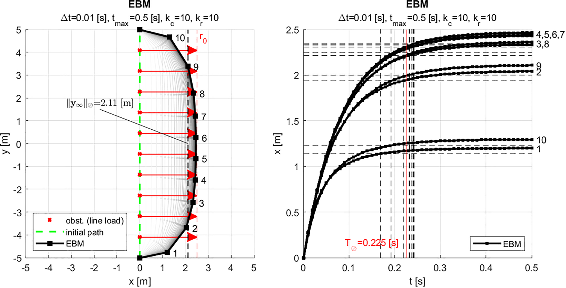
As these geometric shapes are described with only a few parameters, the calculation of the distance $d (p_{i}, h)$ between a single node and the obstacles can be implemented very efficiently. Using the gradient of the scalar force field $H (p_{i}, h) = max (0; r_{0} - d (p_{i}, h))$ , the repulsive force $f_{i} (p_{i}, h) = H (p_{i}, h) \cdot \frac{- \nabla H (p_{i}, h)}{| \nabla H (p_{i}, h) |}$ is numerically evaluated for every node.

On the left side of Figure 11, the scalar force field H is shown for an exemplary static arrangement of three spheric, two capsular, and two planar obstacles represented by its equipotential surfaces. For numerical reasons, the field is additionally smoothed at the transitions between the range of the individual obstacles. On the right side, the evolution of an exemplary path under influence of this field is shown.

Figure 11.

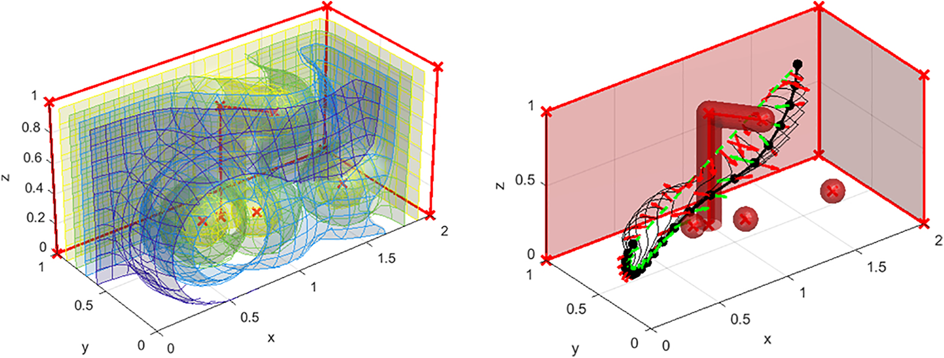
Equipotential surfaces of the scalar force field produced by an exemplary obstacle placement (left) and evolution of an exemplary path within this force field (right).

Results

To validate the method, a test setup with three parallel instances of the CFM each running on an individual industrial control (see Figure 12(a), hard- and software configuration as described in the “Time efficiency” section) and driving a separate UAV was brought into service. The CFM was implemented as a new type of (collision-free) point-to-point interpolation method within these controls. This enabled the use of sequential programs to fly the UAVs to consecutive goals without having to explicitly consider the potential for collisions during programming. For the path interpolation along the nodes, an acceleration-limited motion profile with velocity and acceleration limited to $v_{max} = 1 (m/s)$ and $a_{max} = 0.25 ({m/s}^{2})$ and smoothed node transitions was implemented. The controls were interlinked via a local cloud server to enable a close to real-time exchange of the state data from the UAVs (representing the dynamic obstacles) and to provide information about the remaining static obstacles.⁴³

Because the experimental flights with real UAVs could be carried out only in a secured test cell (see Figure 12(b)), the available workspace for all scenarios was limited to the dimensions of the cell measuring roughly $4 (m) \times 5 (m) \times 4.5 (m)$ . Only the top three meters were used as workspace for flight movements with the CFM. The section underneath was reserved for secure start and landing maneuvers. In addition to the workspace limits that were modeled as planar obstacles, some exemplary peripheral elements within the workspace (e.g. pipelines and supporting structure of the building) were modeled using various capsular obstacles as shown in Figures 14, 15, and 18. All instances of the CFM were parameterized with $n = 20$ , $y_{ϕ, d} = 0.375 (m)$ , and $T_{max, d} = 1 (s)$ resulting in $K = 0.114$ and $T = 0.0454$ . The controls operated at a cycle time of 10 ms and therefore the step size of the CFM was identically set to $Δ t = 0.01 (s)$ .

Figure 12.

Test setup consisting of three industrial controls which are interlinked via a local cloud server (a) and a test cell (b) for secured experimental flights carried out with three lightweight quadcopters (c).

Hardware-in-the-loop simulation

Initially, the controls were set up using a hardware-in-the-loop simulation with both environment and UAVs being simulated. The latter was realized as a state-controlled rigid body model with six degrees of freedom.⁴⁴ Scenario 1 consisted of three simultaneously executed programs with predefined goals that were consecutively approached by the UAVs (see Table 1).

Table 1.

Goal positions for scenario 1 (all coordinates in meters).

	UAV₁			UAV₂			UAV₃
	x	y	z	x	y	z	x	y	z
Initial position (I)	3.2	1	1	1	3.5	0.5	1	1	0.5
Start (S)	3.2	1	2	1	3.5	2	1	1	2
Position 1 (P1)	3.5	3	4.1	3.4	1.2	4	3.5	4	3
Position 2 (P2)	0.5	2	2	2	1	3	1	1	2
Position 3 (P3)	3.2	1	2	1	3.5	2	Not available
Landing (L)	3.2	1	1	1	3.5	0.5	1	1	0.5

The three individual programs were manually started one after the other. Therefore, their execution occurred temporally independent of each other. Figure 13 shows the positions of the individual UAVs in x-, y- and z-direction and the distance d to the closest obstacle over time for an exemplary execution of scenario 1. The position data for actual (bold), desired (fine), and goal (dashed) values are charted. The sections in which the UAVs are in an initial/waiting position or performing a secured start/landing are greyed out and irrelevant for distance and collision monitoring. The zero crossings of d represent the transitions between workspace and the start/landing space.

Figure 13.

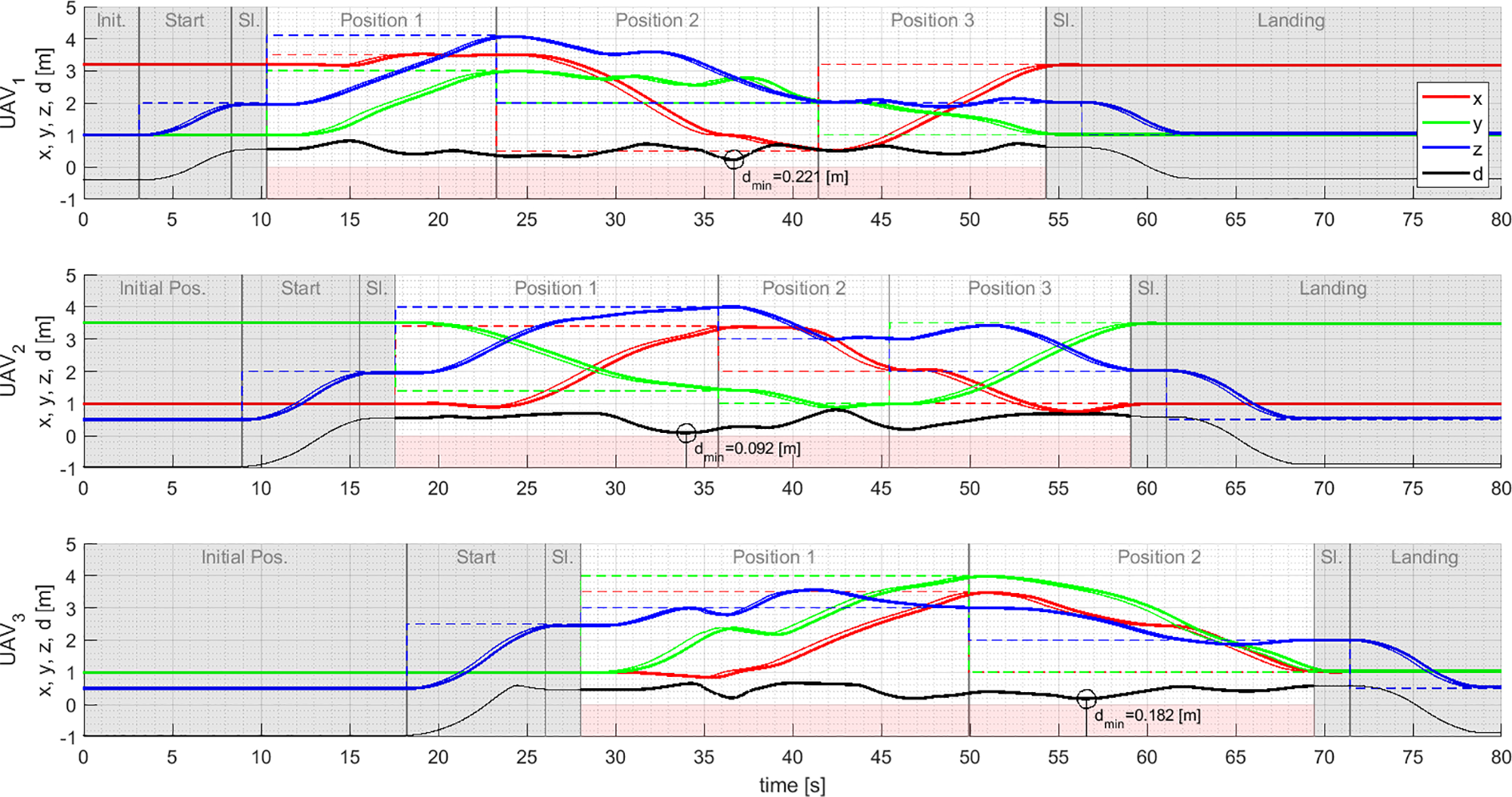
Positions and distances to the closest obstacle over time for scenario 1 with indication of the minimum distance for each UAV. UAV: unmanned aerial vehicle.

Additionally, Figure 14 shows the corresponding three-dimensional trajectories of the actual (bold with marks one second apart) and the desired (fine) positions and Figure 15 shows an excerpt from the online visualization of scenario 1 including the momentary state of the dynamically adjusted global paths.

Figure 14.

Three-dimensional trajectories for scenario 1.

Figure 15.

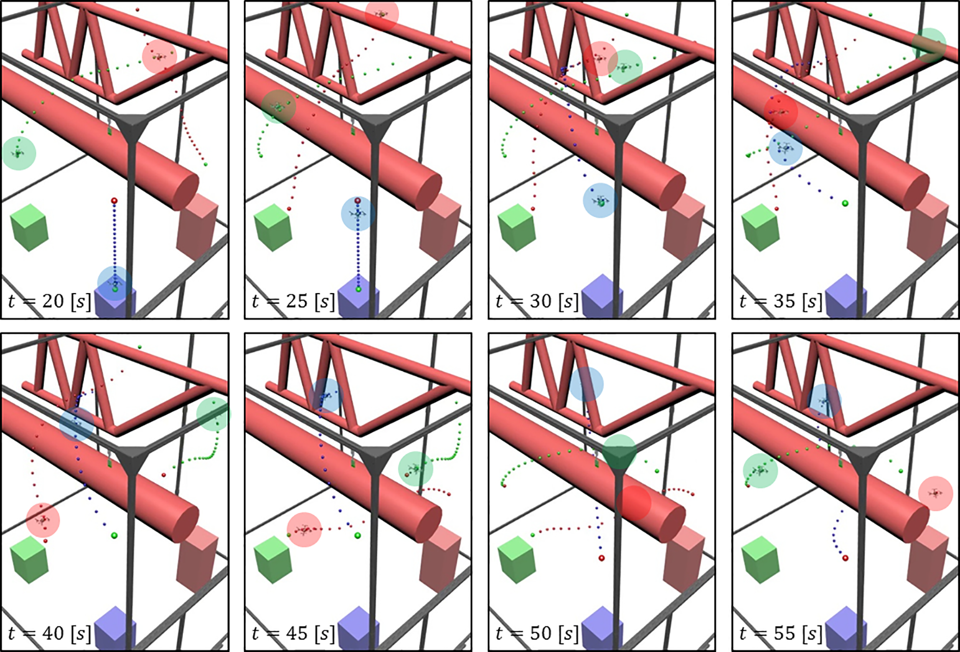
Still images from the online visualization for scenario 1 including the momentary state of the paths dynamically adjusted by the CFM. CFM: curve-shortening flow method.

For scenario 2, several long-term tests were performed with a length of at least 15 min. These consisted of a repetitive cycle with random goals followed by a start and a landing maneuver. Figure 16 shows the timeline for each of the UAVs distance d to the closest obstacle. Start and landing phases which are not relevant to collision monitoring are illustrated using a fine line.

Figure 16.

Distances to the closest obstacle for an exemplary execution of scenario 2.

Real UAVs

Scenario 3 was carried out with real UAVs (Crazyflie 2.0 by Bitcraze, see Figure 12(c)) within the test cell and again predefined goals were used. In concrete, this means that besides the three UAVs themselves, the workspace boundaries were also physically present in this scenario. The remaining static obstacles within the test cell were modeled virtually. As the sensors of the Crazyflie for position detection (Loco Positioning System by Bitcraze in combination with an optical flow sensor) cannot be utilized near walls, the new goals for scenario 3 listed in Table 2 differ from those used in scenario 1.

Table 2.

Goal positions for scenario 3 (all coordinates in meters).

	UAV₁			UAV₂			UAV₃
	x	y	z	x	y	z	x	y	z
Initial Position (I)	3.2	1	1	1	3.5	0.5	1	1	0.5
Start (S)	3.2	1	1.75	1	3.5	1.75	1	1	1.75
Position 1 (P1)	1.2	4	2	2.5	1.4	2.8	2.6	3.75	3.2
Position 2 (P2)	1.2	2	2	1	3.5	1.75	1	1	1.75
Position 3 (P3)	3.2	1	1.75	Not available			Not available
Landing (L)	3.2	1	1	1	3.5	0.5	1	1	0.5

Figure 17 shows the position and the distance to the closest obstacle over time for an exemplary execution of scenario 3. Figure 18 shows the corresponding three-dimensional paths of the actual and desired positions. Additionally, Figure 19 shows the paths of the actual positions tracked by a camera.

Figure 17.

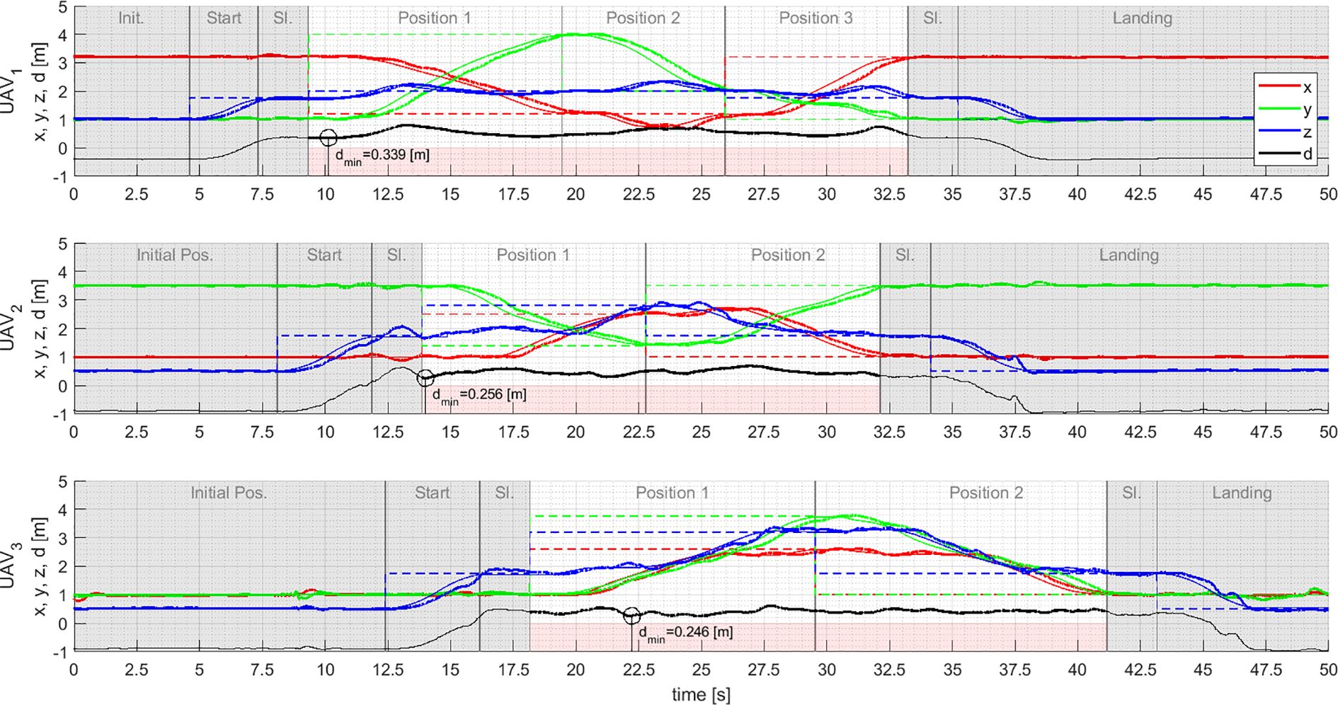
Positions and distances to the closest obstacle over time for scenario 3 with indication of the minimum distance for each UAV. UAV: unmanned aerial vehicle.

Figure 18.

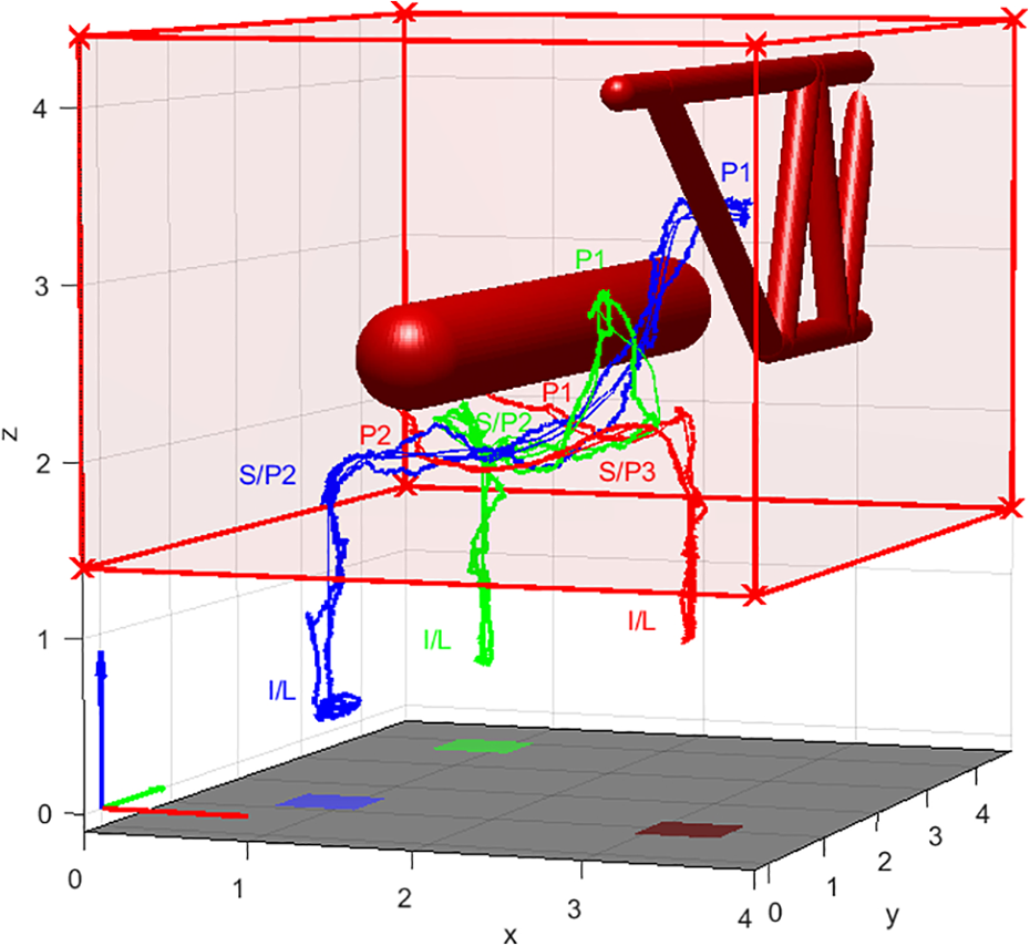
Three-dimensional paths for scenario 3 (tracked with Loco Positioning System).

Figure 19.

Three-dimensional paths with marks 5 s apart for scenario 3 (tracked with camera).

Scenarios 1 and 2 demonstrated the ability of the CFM to autonomously generate reference trajectories that continuously adapt to the environment’s current state for independently triggered flight movements. The resulting distance timelines show the absence of collisions of the actual trajectories flown by the UAVs. Besides proving the functionality of the CFM, scenarios 1 and 2 also evidence that the CFM is implementable on industrial hardware under real-time conditions with cycle times of only a few milliseconds. In addition, scenario 3 proves the applicability of the CFM for real UAVs.

Conclusion

In this article, the CFM was introduced as a new method for online path planning in dynamic environments. The CFM was theoretically derived and compared to the functionally similar EBM. It was shown that the CFM has improved numerical robustness, parameterability, and computational efficiency. Several validation scenarios with three interlinked instances of the CFM for control of UAVs in the context of intralogistics were performed. The autonomously generated and collision-free trajectories of the UAVs thereby proved the functionality of the CFM and demonstrated its executability on industrial hardware in real-time.

Footnotes

Acknowledgements

The authors would like to thank the Institute for Control Engineering of Machine Tools and Manufacturing Units at the University of Stuttgart directed by Prof. Alexander Verl for their support within this project.

Declaration of conflicting interests

The author(s) declared no potential conflicts of interest with respect to the research, authorship, and/or publication of this article.

Funding

The author(s) disclosed receipt of the following financial support for the research, authorship, and/or publication of this article: This work has been granted by the German Research Foundation within the project numbers 50131014 and 189927270. Further financial support has been provided by the University of Applied Sciences Esslingen, Aalen University, and the Baden Wuerttemberg Ministry of Economy, Labor and Housing within the Transfer Platform Industry-4.0. The article processing charge was funded by the Baden-Wuerttemberg Ministry of Science, Research and Culture and the University of Applied Sciences Esslingen in the funding programme Open Access Publishing.

ORCID iD

Marcel Huptych

References

Kunz

Reiser

Stilman

, et al. Real-time path planning for a robot arm in changing environments. In: 2010 IEEE/RSJ international conference on intelligent robots and systems (IROS), Taipei, Taiwan, 18–22 October 2010, pp. 5906–5911. IEEE.

Borenstein

Koren

. Real-time obstacle avoidance for fast mobile robots. IEEE Trans Syst Man Cybern 1989; 19(5): 1179–1187.

Borenstein

Koren

. The vector field histogram-fast obstacle avoidance for mobile robots. IEEE Trans Robot Autom 1991; 7(3): 278–288.

Ulrich

Borenstein

. VFH+: reliable obstacle avoidance for fast mobile robots. In: Proceedings. 1998 IEEE international conference on robotics and automation, 16–20 May 1998, Leuven, Belgium, pp. 1572–1577. IEEE.

Ulrich

Borenstein

. VFH: local obstacle avoidance with look-ahead verification. In: Proceedings 2000 ICRA. Millennium conference. IEEE international conference on robotics and automation. Symposia proceedings (Cat. No. 00CH37065), 24–28 April 2000, San Francisco, USA, pp. 2505–2511. IEEE.

Minguez

Montano

. Nearness diagram (ND) navigation: collision avoidance in troublesome scenarios. IEEE Trans Robot Autom 2004; 20(1): 45–59.

Fox

Burgard

Thrun

. The dynamic window approach to collision avoidance. IEEE Robot Autom Mag 1997; 4(1): 23–33.

Khatib

. Real-time obstacle avoidance for manipulators and mobile robots. In: Proceedings. 1985 IEEE international conference on robotics and automation, St. Louis, MO, USA, 25–28 March 1985, pp. 500–505. IEEE.

Goerzen

Kong

Mettler

. A survey of motion planning algorithms from the perspective of autonomous UAV guidance. J Intell Robot Syst 2010; 57: 65–100.

10.

Koren

Borenstein

. Potential field methods and their inherent limitations for mobile robot navigation. In: Proceedings. 1991 IEEE international conference on Robotics and automation, Sacramento, CA, USA, 9–11 April 1991, pp. 1398–1404. IEEE.

11.

Koditschek

. Exact robot navigation by means of potential functions: some topological considerations. In: Proceedings. 1987 IEEE international conference on robotics and automation, Raleigh, NC, USA, 31 March–3 April 1987, pp. 1–6. IEEE.

12.

LaValle

Kuffner

Jr . Randomized kinodynamic planning. Int J Robot Res 2001; 20: 378–400.

13.

Kavraki

Svestka

Latombe

, et al. Probabilistic roadmaps for path planning in high-dimensional configuration spaces. IEEE Trans Robot Autom 1996; 12(4): 566–580.

14.

Otte

Frazzoli

. RRT X: real-time motion planning/replanning for environments with unpredictable obstacles. In: Akin

Amato

Isler

van der Stappen

(eds) Algorithmic foundations of robotics XI. Cham: Springer, 2015, pp. 461–478.

15.

Naderi

Rajamäki

Hämäläinen

. RT-RRT: a real-time path planning algorithm based on RRT. In: Proceedings of the 8th ACM SIGGRAPH conference on motion in games, 16–18 November 2015, Paris, France, pp. 113–118. ACM.

16.

Kallman

Mataric

. Motion planning using dynamic roadmaps. In: Proceedings. ICRA’04. 2004 IEEE international conference on robotics and automation, 2004, New Orleans, LA, USA, 26 April–1 May 2004, Citeseer, pp. 4399–4404.

17.

Leven

Hutchinson

. A framework for real-time path planning in changing environments. Int J Robot Res 2002; 21: 999–1030.

18.

Yang

Brock

. Elastic roadmaps—motion generation for autonomous mobile manipulation. Auton Robot 2010; 28: 113–130.

19.

Likhachev

Gordon

Thrun

. ARA: formal analysis. Tech. Rep. CMU-CS-03-148, Carnegie Mellon University, Pittsburgh, PA, 2003.

20.

Koenig

Likhachev

. D Lite. In: Proceedings AAAI National Conferenceon Artificial Intelligence, 28 July – 1 August 2002, Edmonton, Alberta, Canada, pp. 476–483.

21.

Kuwata

Teo

Fiore

, et al. Real-time motion planning with applications to autonomous urban driving. IEEE Trans Control Syst Technol 2009; 17(5): 1105–1118.

22.

Benenson

Petti

Fraichard

, et al. Integrating perception and planning for autonomous navigation of urban vehicles. In: 2006 IEEE/RSJ international conference on intelligent robots and systems, Beijing, China, 9–15 October 2006, pp. 98–104.

23.

Hrabar

. Reactive obstacle avoidance for rotorcraft UAVs. In: 2011 IEEE/RSJ international conference on intelligent robots and systems (IROS), San Francisco, CA, USA, 25–30 September 2011, pp. 4967–4974.

24.

Hrabar

. 3D path planning and stereo-based obstacle avoidance for rotorcraft UAVs. In: IEEE/RSJ international conference on intelligent robots and systems, 2008. IROS 2008, Nice, France, 22–26 September 2008, pp. 807–814. IEEE.

25.

Quinlan

Khatib

. Elastic bands: connecting path planning and control. In: Proceedings. 1993 IEEE international conference on robotics and Automation, 1993, Atlanta, GA, USA, 2–6 May 1993, pp. 802–807. IEEE.

26.

Brock

Khatib

. Elastic strips: a framework for motion generation in human environments. Int J Robot Res 2002; 21: 1031–1052.

27.

Quinlan

. Real-time modification of collision-free paths. Stanford, CA: Stanford University, 1994.

28.

Philippsen

. Motion planning and obstacle avoidance for mobile robots in highly cluttered dynamic environments. PhD thesis, EPFL, Lausanne, Switzerland, 2004.

29.

Graf

Hans

Schraft

. Care-O-bot II—development of a next generation robotic home assistant. Auton Robot 2004; 16: 193–205.

30.

Graf

Parlitz

Hägele

. Robotic home assistant care-o-bot 3 product vision and innovation platform. In: International conference on human-computer interaction, Tokyo, Japan, 23–25 November 2009, pp. 312–320. Springer.

31.

Brandt

Sattel

. Path planning for automotive collision avoidance based on elastic bands. In: Proceedings of the 16th IFAC World Congress, Prague, Czech Republic, 3–8 July 2005, pp. 210–215.

32.

Chow

Glickenstein

. Semidiscrete geometric flows of polygons. Am Math Mont 2007; 114: 316–328.

33.

Devadoss

O’Rourke

. Discrete and computational geometry. Princeton: Princeton University Press, 2011.

34.

Chou

Zhu

. The curve shortening problem. Boca Raton: Chapman and Hall/CRC, 2001.

35.

Noschese

Pasquini

Reichel

. Tridiagonal Toeplitz matrices: properties and novel applications. In: Numerical linear algebra with applications (ed. Vassilevski

), 2013, Vol. 20, Issue 2, pp. 302–326. Wiley.

36.

Levine

. The control handbook. Florida: CRC press, 1996.

37.

Plato

. Numerische Mathematik kompakt. 2000. Wiesbaden, Germany: Springer.

38.

Golub

Van Loan

. Matrix computations. Baltimore: Johns Hopkins University Press, 1996.

39.

Thomas

. Elliptic problems in linear difference equations over a network. New York: Watson Sci. Comput. Lab. Rept., Columbia University, 1949.

40.

Kanzow

. Numerik linearer Gleichungssysteme: direkte und iterative Verfahren. Wiesbaden, Germany: Springer-Verlag, 2007.

41.

McMahon

. The Livermore Fortran Kernels: a computer test of the numerical performance range. Livermore, CA: Lawrence Livermore National Lab., 1986.

42.

Hwang

Ahuja

. Gross motion planning—a survey. ACM Comput Surveys (CSUR) 1992; 24: 219–291.

43.

von Bergen

Huptych

Röck

. Autonome Flugrobotik für die wandlungsfähige Fabrik—Steuerung, Infrastruktur und Simulation. wt-online, 2018, pp. 834–839.

44.

Kurak

Hodzic

. Control and estimation of a quadcopter dynamical model. Periodicals of Eng Natural Sci 2018; 6: 63–75.

Real-time path planning in dynamic environments for unmanned aerial vehicles using the curve-shortening flow method

Abstract

Keywords

Introduction

Related work

Curve-shortening flow method

Mathematical description

Parameter influence

Analytical parameterization

Path dynamics

Stationary displacement

Calculation of the repulsion parameter

Calculation of the dynamics parameter

Time discretization

Comparison to elastic bands method

Path behavior equalization

Numerical robustness

Time efficiency

Improvements

Modeling of the environment

Results

Hardware-in-the-loop simulation

Real UAVs

Conclusion

Footnotes

Acknowledgements

Declaration of conflicting interests

Funding

ORCID iD

References