Sage Journals: Discover world-class research

Abstract

A tensegrity is a self-stressed pin-jointed system consisting of tensile members and compressive members. As its shape can be actively controlled by changing the prestress of its members, it has great potential to be used as a shape-controllable locomotive system. Particularly, the six-strut spherical tensegrity has been studied intensively as a rolling locomotive system. In this study, the rolling gaits of a strut-actuated six-strut spherical tensegrity are investigated. Specifically, a mathematical model for generating the rolling gaits of locomotive spherical tensegrities is presented, and a numerical method combining dynamic relaxation method and genetic algorithm is used to solve the model. Various rolling gaits for the strut-actuated six-strut locomotive spherical tensegrity are identified using this approach. Two basic types of touching-ground triangles, two basic distributions of payload, and six cases for the numbers of used active struts are considered. Several rolling gait primitives are noted, their motion features analyzed, and a simple path-generating strategy is proposed based on idealized rolling gait primitives. A physical prototype of the strut-actuated six-strut locomotive tensegrity is manufactured, and experiments are conducted to verify the rolling gaits and locomotion paths generated by the proposed methods.

Keywords

Locomotive tensegrity six-strut spherical tensegrity rolling gait path planning experimental validation

Introduction

A tensegrity system is a special pin-jointed structural system that consists of a set of discontinuous compressive components interacting with a set of continuous tensile components to define a stable volume in space.¹ A distinguishing feature of the tensegrity is that its shape can be actively controlled by the prestress in the members, which makes it a good candidate for structural systems requiring controllable shapes, such as smart structures,^2,3 deployable structures,^4,5 and locomotive robots.^6
–8

Much attention has been paid to locomotive tensegrity systems recently, with two being of particular interest: the spine-like tensegrity system⁹ and the spherical tensegrity system.¹⁰ Orki et al.¹¹ proposed a caterpillar-like robot based on a planar tensegrity system and investigated its crawling gaits and control strategies. Bliss et al.¹² experimentally validated the bio-inspired control of a fish-like tensegrity robot. Frison et al.^13,14 presented a tensegrity robot named duct climbing tetrahedral tensegrity, which was able to climb on the wall of a pipe for duct cleaning. Tietz et al.¹⁵ studied a spine-like tensegrity robot, tetraspine, composed of rigid tetrahedron-shaped units connected by six strings. Shibata et al.¹⁶ proposed a deformable robot based on a six-strut tensegrity, which was able to crawl by body deformation. Koizumi et al.¹⁷ proposed and experimentally tested a six-strut tensegrity robot whose 24 tensile components were replaced by pneumatic soft actuators. Kim¹⁸ created four prototypes of spherical tensegrity robots based on 6-rod and 12-rod tensegrity systems and studied the robots’ rolling and hopping locomotion. Khazanov et al.¹⁹ proposed a new concept that used vibration to locomote tensegrity systems, and the feasibility and advantages of this new concept were preliminarily verified using a small-scale physical prototype using a six-strut tensegrity installed with three controlled vibration motors. Many studies have also been undertaken on spherical tensegrity robots in an attempt to identify their potential application to planetary exploration.^20

–23

However, most of the existing research on locomotive tensegrity systems focuses on the locomotion gaits themselves, and little work has been undertaken on the method for generating locomotion gaits. In this study, the rolling gaits of a strut-actuated six-strut spherical tensegrity are studied. A method using both a mathematical model and a genetic algorithm (GA)-based approach is proposed to generate rolling gaits for the locomotive tensegrity. The effects of the type of touching-ground triangles, the distribution of the payload, and the number of active members on the rolling gaits are considered. Several rolling gait primitives are identified, and their characteristics are analyzed and discussed in detail.

Generating of rolling gaits

The rolling gait of a locomotive spherical tensegrity system is a motion that mimics the rolling of spheres. A conceptual demonstration of this motion is shown in Figure 1. A spherical tensegrity system is in a static equilibrium state at the initial position, but the centroid of the system changes because of the structural deformation controlled by actuators. As the deformation increases, the system cannot maintain its equilibrium in the initial position and rolls to a new position. In the new position, the static equilibrium is reached again and, if the deformation caused by the external load and gravity is ignored, the system reverts to its original form to prepare for the next cycle of gait motion.

Figure 1.

Mechanism of rolling gait.

Mathematical model

A locomotive tensegrity system with n nodes, n_c members, n_a active members, and n_r degrees of freedom is considered here. The types of structural members are indexed by the vector $D = [D_{1}, D_{2}, \dots, D_{n_{c}}]$ , where D_i = 0 if the ith member is a tensile member and D_i = 1 if the ith member is a compressive member. The locations of active members are indexed by the vector $D_{a} = [D_{a} _{1}, D_{a} _{2}, \dots, D_{a n_{c}}]$ , where D_ai = 0 if the ith member is a passive member and D_ai = 1 if the ith member is an active member. The sum of the components of D _a is equal to the number of active members n_a .

The control strategy of a locomotive tensegrity system can be described by an actuating function Δ. During a given time period [t_s, t_f ], the actuating function of the ith member is defined as e_i = f_i (t), where f_i is a function of time t. The actuating function Δ is written as

Δ = \{e_{1}, e_{2}, \dots, e_{n_{c}}\}

where e_i = 0 for a passive member and $e_{i} \in [- e_{i}^{s}, e_{i}^{l}]$ for an active member. $e_{i}^{s}$ and $e_{i}^{l}$ are the allowable shortening and elongation of the active member, respectively.

The rest length of members $L_{R}^{t}$ at time t satisfies

L_{R}^{t} = L_{R}^{t_{s}} + Δ^{t}

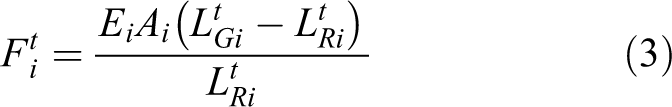
The internal force $F_{i}^{t}$ of the ith member is determined by

F_{i}^{t} = \frac{E_{i} A_{i} (L_{G i}^{t} - L_{R i}^{t})}{L_{R i}^{t}}

where E_i , A_i , $L_{G i}^{t}$ , and $L_{R i}^{t}$ are the elasticity modulus, cross-sectional area, geometry length, and rest length of the ith member, respectively. Meanwhile, the internal force $F_{i}^{t}$ of the ith member is required to be within the strength limitations, that is

\begin{array}{l} - min (F_{c i}, F_{b i}) \leq F_{i}^{t} \leq 0, for D_{i} = 1 \\ 0 \leq F_{i}^{t} \leq F_{t i}, for D_{i} = 0 \end{array}

where F_ci , F_bi , and F_ti are the compressive strength, buckling strength, and tensile strength of the ith member, respectively.

The unbalanced nodal force R ^t of the system at time t can be expressed as

R^{t} = F_{L}^{t} - A^{t} F^{t}

where $F_{L}^{t}$ , $A^{t}$ , and $F^{t}$ are the vector of nodal loads, the matrix of equilibrium, and the vector of member internal forces, respectively. Note that the component of $F^{t}$ is determined by equation (3). The component of A^t can be determined by the nodal coordinates.²⁴

According to Newton’s second law

R^{t} = M \overset{​}{{\ddot{U}}^{t}} + C {\dot{U}}^{t}

where M is the nodal mass matrix of the system, C is the viscous damping of the system, and U is the matrix of nodal coordinates of the system.

Substituting equation (5) into equation (6) yields

F_{L}^{t} - A^{t} F^{t} = M \overset{​}{{\ddot{U}}^{t}} + C {\dot{U}}^{t}

As mentioned above, the rolling gait considered in this study starts and ends with a static equilibrium, that is

{\dot{U}}^{t_{s}} = {\dot{U}}^{t_{f}} = 0, \overset{​}{{\ddot{U}}^{t_{s}}} = \overset{​}{{\ddot{U}}^{t_{f}}} = 0

To ensure that the final form of the system recovers to the initial form if the deformation caused by the external load and gravity is ignored, the rest lengths of members at the final state (t = t_f ) are required to be identical to those at the start state (t = t_s ), that is

e_{i}^{t_{f}} = e_{i}^{t_{s}}

The objective function G(Δ) is defined to maximize the horizontal motion of the centroid of the system generated by the gait, that is

G (Δ) = \frac{1}{{‖ U_{c x y}^{t_{f}} - U_{c x y}^{t_{s}} ‖}_{2}}

where $U_{c x y}^{t_{f}}$ and $U_{c x y}^{t_{s}}$ are the projections of the coordinates of the centroid on the horizontal plane xy.

The problem of finding the optimal rolling gaits for the locomotive tensegrity system can be formulated as

\{\begin{cases} find Δ = \{e_{1}, e_{2}, \dots, e_{n_{c}}\} \\ min G (Δ) \\ s . t . : \\ U \in Ω, {\dot{U}}^{t_{s}} = {\dot{U}}^{t_{f}} = 0, \overset{​}{{\ddot{U}}^{t_{s}}} = \overset{​}{{\ddot{U}}^{t_{f}}} = 0 \\ F_{L}^{t} - A^{t} F^{t} = M \overset{​}{{\ddot{U}}^{t}} + C {\dot{U}}^{t} \\ i = 1, 2, \dots, n_{c} \\ e_{i} \in [- e_{i}^{s}, e_{i}^{l}], for D_{a i} = 1 \\ e_{i} = 0, for D_{a i} = 0 \\ - min (F_{c i}, F_{b i}) \leq F_{i}^{t} \leq 0, f o r D_{i} = 1 \\ 0 \leq F_{i}^{t} \leq F_{t i}, f o r D_{i} = 0 \\ e_{i}^{t_{f}}, e_{i}^{t_{s}} \end{cases}

Here, $Ω$ represents the free space in the environment where the locomotive system does not interfere with boundaries or obstacles.

Numerical method

To evaluate the feasibility of a given control strategy, the response of the system under the given strategy needs to be tracked, that is, equation (7) must be solved under a given Δ ^t at $t \in [t_{s}, t_{f}]$ . In this study, an incremental dynamic relaxation method (DRM) combined with an internal collision-detecting algorithm is used to track and judge the feasibility of the motion path of the locomotive spherical tensegrity. The effectiveness of this method in the path tracking of controlled tensegrity systems has been verified in previous studies.^25,26 Note that virtual nodal mass, sectional stiffness of members, and damping were used for the DRM in previous studies where the response of the structural system was deemed to be quasi-static. While dynamic responses must be considered in this study and thus real values of these variables are used here.

The contact between the nodes of the tensegrity and the ground is evaluated by the penalty function.²⁷ A virtual spring with stiffness k_n is assumed, and the normal contact force F_n and the maximum friction force F_f are evaluated by

\begin{array}{l} F_{n} = k_{n} δ \\ F_{f} = μ F_{n} \end{array}

where δ is the penetration depth and μ is the friction coefficient.

The gait-generating problem equation (11) is a typical combinatorial optimization problem, and its solution domain is generally large. Stochastic search algorithms, such as GA,²⁸ simulated annealing,²⁹ and evolutional algorithms,³⁰ have been verified suitable for problems such as these. Here, a GA is adopted to search for the optimal rolling gait, and its fitness function is defined as 1/G(Δ).

Figure 2 shows the flow chart of the optimization searching for rolling gaits. This algorithm is programmed and implemented using the commercial software MATLAB.³¹ The main steps are as follows:

Define the genetic representation, and the fitness function, and initialize a population.

Decode the chromosomes.

For each individual, build the numerical model of the tensegrity system for the DRM; initialize the parameters of the numerical tensegrity model and set t = t_s ; and then conduct step (4) to step (6).

Apply a control strategy on the numerical tensegrity model through the actuating function Δ ^t .

Calculate the residual nodal force R ^t ; solve equation (7) using the central difference method; update the nodal acceleration ${\ddot{U}}^{t}$ , velocity ${\dot{U}}^{t_{}}$ , and coordinate U ^t and apply constraints.

If t = t _f, go to step (7); otherwise, set t = t + Δt and go to step (4).

Evaluate the fitness of the population. If the population satisfies the convergence condition or the number of generations reaches the maximum allowed number, go to step (9); otherwise, go to step (8).

Apply the selection, crossover, and mutation operators and generate a new generation. Then go to step (2).

Record the solutions.

Figure 2.

Flow chart of optimization searching of rolling gaits.

Strut-actuated six-strut spherical tensegrity

As shown in Figure 3, a six-strut spherical tensegrity is composed of the 6 struts, 12 nodes, and 24 tendons. Each node is connected to a strut and four tendons. The six struts are divided into three pairs, and the struts in each pair are parallel to each other. The outside surface of the six-strut tensegrity is an icosahedron that consists of 8 closed triangles (TCs) and 12 open triangles (TOs). A TC has three tendon edges, and a TO has two tendon edges. As listed in Table 1, these triangles are numbered for the convenience of rolling gait descriptions. According to the types of triangles touching the ground, there are two basic states for the tensegrity: TC state and TO state, as shown in Figure 3. To ensure the repeatability of the rolling gaits, the start state and final state of the tensegrity before and after a rolling gait are required to be identical to one of the basic states. The struts are used as active members whose rest lengths can be actively changed by actuators, and they are labeled with the prefix “A” in Figure 3(a). The properties assumed for the active struts and tendons are given in Table 2.

Figure 3.

Six-strut spherical tensegrity: (a) TC state and (b) TO state. TC: closed triangle; TO: open triangle.

Table 1.

Number of triangles.

Type	Triangle number	Nodes
TC–	1	1, 5, 10
	2	1, 8, 9
	3	2, 5, 11
	4	2, 8, 12
	5	3, 6, 11
	6	3, 7, 12
	7	4, 6, 10
	8	4, 7, 9
TO–	1	1, 2, 5
	2	1, 2, 8
	3	1, 9, 10
	4	2, 11, 12
	5	3, 11, 12
	6	3, 4, 6
	7	3, 4, 7
	8	4, 9, 10
	9	5, 6, 10
	10	5, 6, 11
	11	7, 8, 9
	12	7, 8, 12

TC: closed triangle; TO: open triangle.

Table 2.

Properties of members.

Properties	Struts	Tendons
Initial rest length (m)	0.2	0.12
Mass (kg)	0.065	0.001
Stiffness (N/m)	2 × 10⁵	205
Prestress (N)	−31.36	12.8
Compressive strength (N)	−150	0
Tensile strength (N)	150	150

The allowable shortening and elongation lengths, $e_{i}^{s}$ and $e_{i}^{l}$ , of the actuated struts are assumed to be 4.7 and 5.3 cm, respectively. The actuated struts are assumed to be able to change their rest lengths at a speed of 5 mm/s. The damping ratio is set as 0.01, the gravity acceleration is 9.8 m/s², and the coefficient of friction is set as 0.5.

Because of the symmetry of the tensegrity, rolling gaits can be classified by the type of touching-ground triangles. Therefore, the effect of the type of touching-ground triangles is investigated. The locomotive tensegrity carries some payload for potential applications, and the payload can be either distributed or lumped. The distributed payload is assumed to act uniformly on the nodes, and the lumped payload is assumed to apply to the system by suspending an object to the 12 nodes with 12 additional tendons. The object is located at the centroid of the system in the basic states. Our study considers a total payload of 151.6 g and a structural weight of 446.9 g. Although all the struts can be actuated, there may be gaits using less than six and, therefore, the effect of the number of active struts used is studied. The cases or values for the above parameters are given in Table 3.

Table 3.

Cases or values for parameters.

Parameters	Cases/values
Touching-ground triangle	TO and TC
Distribution of payload	Distributed and lumped
Number of actuated struts used	1, 2, 3, 4, 5, 6

TC: closed triangle; TO: open triangle.

Rolling gaits

Summary of gait-generating results

To search for the optimal rolling gaits for the six-strut locomotive tensegrity system, the parameters of the GA are set as follows: the population size is 50; the maximum allowed generation is 100; and the generation gap, crossover rate, and mutation rate are 0.8, 0.7, and 0.01, respectively. Twenty-four computations using different sets of parameters given in Table 3 are conducted. The maximum fitness versus generation curves of the computations are shown in Figure 4. Note that the fitness represents the traveling distance generated by the gait.

Figure 4.

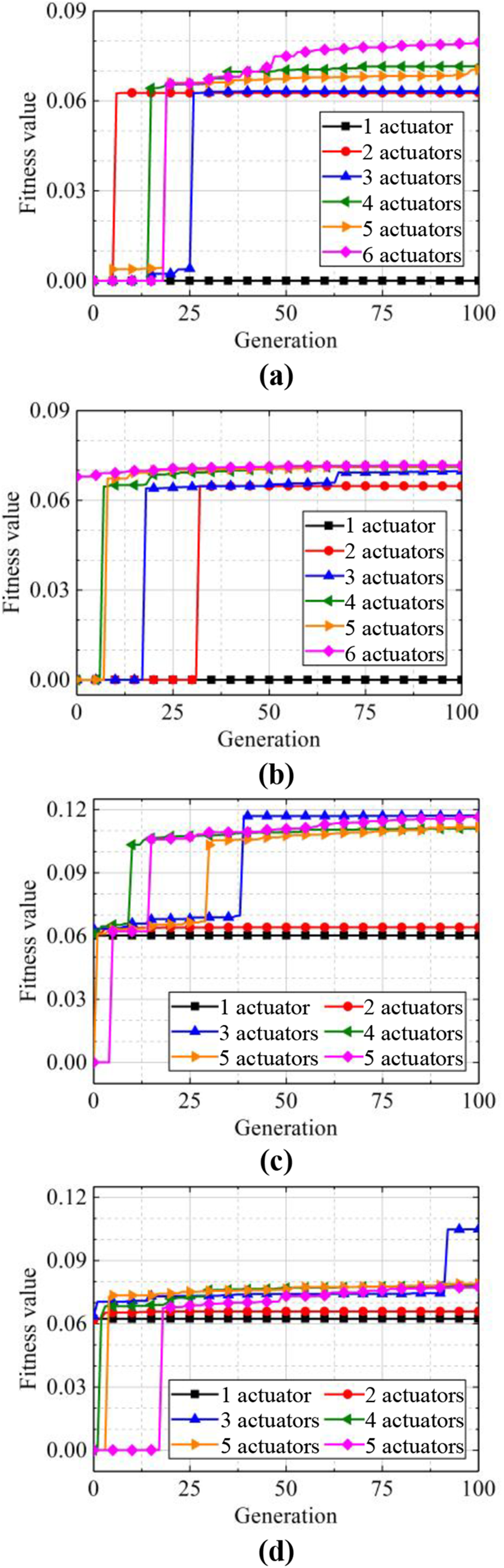
Fitness versus generation: (a) TC state with distributed payload; (b) TC state with lumped payload; (c) TO state with distributed payload; and (d) TO state with lumped payload. TC: closed triangle; TO: open triangle.

It is observed that the maximum fitness for the cases in a TC state remains at zero when only one actuated strut is used (Figure 4(a) and (b)). This observation indicates that no rolling gait using only one actuated strut can be found in a TC state. For the other cases, gaits with a traveling distance of more than 0.06 m are found within 40 generations. The maximum fitness achieved by the cases in a TC state is approximately 0.08 (Figure 4(a)) and that achieved by the cases in a TO state is approximately 0.12 (Figure 4(c)). This shows that the maximum traveling distance achieved by the gaits starting from a TO state is greater than that achieved by the gaits starting from a TC state. It also suggests that the maximum traveling distance achieved by the gait of a system with a distributed payload is larger than that achieved by the gait of a system with a lumped payload (Figure 4).

Rolling gait primitives

Several rolling gait primitives can be identified from these results, as listed in Table 4. In this table, a rolling gait primitive is notated by the initial and final touching-ground triangles. For example, TC–6→TO–5 notates a gait rolling from TC–6 to TO–5. This notation is used throughout the article. Various control strategies can realize each rolling gait primitive, and a typical control strategy for each, together with the corresponding traveling distance, is given in Table 4.

Table 4.

Rolling gait primitives and typical control strategies.

Payload distribution	No.	Rolling gait primitives	Traveling distance (cm)	Actuation length (cm)
Payload distribution	No.	Rolling gait primitives	Traveling distance (cm)	1	2	3	4	5	6
Distributed	1	TC–6→TO–5	6.26	−4.39	5.20	—	—	—	—
	2	TC–6→TO–7	6.27	5.30	—	−3.94	—	—	—
	3	TC–6→TO–12	6.27	—	−3.94	5.30	—	—	—
	4	TO–5→TC–5	6.03	5.30	—	—	—	—	—
	5	TO–5→TC–6	6.27	—	—	—	—	—	5.30
	6	TO–5→TC–5→TO–6	11.71	5.30	—	−4.65	—	—	3.85
	7	TO–5→TC–5→TO–10	10.54	5.24	−3.79	5.05	−4.28	—	—
	8	TO–5→TC–6→TO–12	10.78	−4.65	−3.74	5.12	−4.28	—	—
Lumped	9	TC–6→TO–5	6.48	−4.22	5.28	—	—	—	—
	10	TC–6→TO–7	6.48	5.30	—	−4.15	—	—	—
	11	TC–6→TO–12	6.41	—	−4.67	4.84	—	—	—
	12	TO–5→TC–5	6.24	5.30	—	—	—	—	—
	13	TO–5→TC–6	6.27	—	—	—	—	—	5.30
	14	TO–5→TC–6→TO–12	10.48	—	−4.56	3.73	—	—	5.28

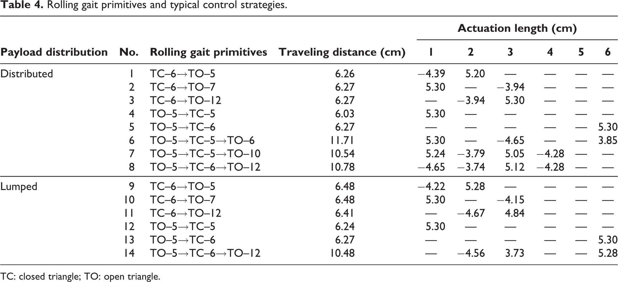
TC: closed triangle; TO: open triangle.

In the rolling gait primitives starting with a TC state, the tensegrity primarily rolls to the adjacent TOs, that is, TC–6→(TO–5, TO–7, or TO–12), as shown in Figure 5(a). The locomotion directions of the rolling gaits starting with a TC state are plotted in Figure 5(b). Three main ranges, namely 95°–105°, 214°–225°, and 335°–341°, are covered by these locomotion directions, and these ranges take up approximately 8.3% of a full circle. The intervals of the three main directions are approximately 120°, indicating the rotational symmetry of the tensegrity.

Figure 5.

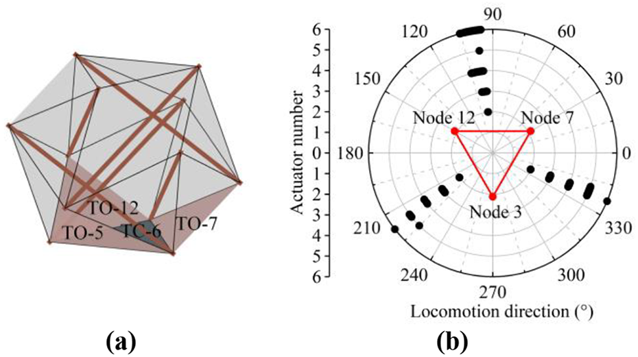
Rolling gaiting starting with a TC state: (a) starting state and (b) locomotion directions. TC: closed triangle.

In the rolling gait primitives starting with a TO state, the tensegrity primarily rolls to the adjacent TCs, that is, TO–5→(TC–5 or TC–6), as shown in Figure 6(a). Secondary rolling occurs in some cases, that is, TO–5→TC–5→(TO–6 or TO–10) and TO–5→TC–6→TO–12. The typical traveling distance of a gait with secondary rolling is significantly larger than that of a gait without secondary rolling. This explains the above observation that the maximum traveling distance being achieved by the rolling gaits starting with a TO state is greater than that being achieved by the rolling gaits starting with a TC state. The locomotion directions of the rolling gaits starting with a TO state are plotted in Figure 6(b). Two direction ranges, that is, 19°–44° and 245°–269°, are covered by the gaits without secondary rolling, and another two direction ranges, that is, 63°–73° and 212°–223°, are covered by the gaits with secondary rolling. These direction ranges take up approximately 20.9% of a full circle.

Figure 6.

Rolling gaiting starting with a TO state: (a) starting state and (b) locomotion directions. TO: open triangle.

Table 4 also presents that all the rolling gait primitives starting with a TC state are single-rolling, and all the double-rolling gait primitives start with a TO state.

Rolling axis

Examination of the detailed dynamic process of the rolling gaits shows that some gaits roll the system around a fixed axis, whereas others roll the system around a moving axis. The motion of the rolling axis causes the traveling distance and motion direction of a gait to deviate from the analytical estimations based on geometrically unfolding the triangle faces.

The rolling gait TC–6→TO–5 using the typical control strategy given in Table 4 is taken as an example of gaits rolling around a fixed axis. In this gait, the system rolls from TC–6 (3, 7, 12) to TO–5 (3, 11, 12), as shown in Figure 7(a). The projections of the motion trajectories of the centroid and some typical nodes on the ground are shown in Figure 8(a). The rolling axis is along the tendon connecting nodes 3 and 12. The displacement of nodes 3 and 12 is very slight and, therefore, the rolling axis can be considered to be fixed. The centroid moves from the right to the left of the rolling axis (Figure 8(a)) with significant motion displayed by nodes 7 and 11 (Figure 8(a)).

Figure 7.

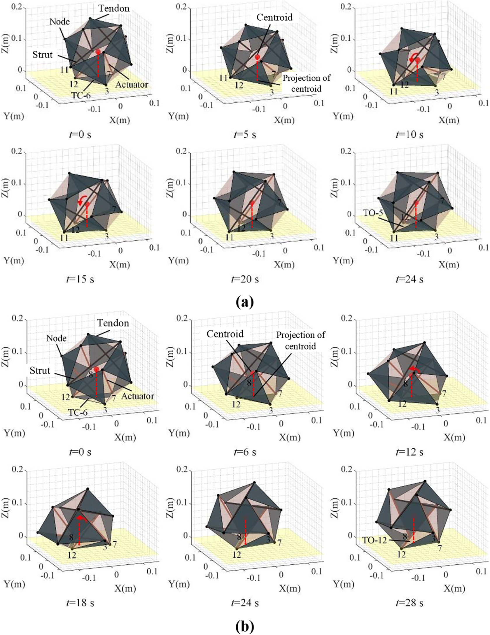
Travel of tensegrity rolling around (a) a fixed axis and (b) a moving axis.

Figure 8.

Projection of nodes and centroid of tensegrity rolling around (a) fixed axis and (b) moving axis.

The rolling gait TC–6→TO–12 using the typical control strategy given in Table 4 is taken as an example of gaits rolling around a moving axis. In this gait, the system rolls from TC–6 (3, 7, 12) to TO–12 (7, 8, 12), as shown in Figure 7(b). The projections of the corresponding motion trajectories of the centroid and some typical nodes on the ground are shown in Figure 8(b). The rolling axis is along the tendon connecting nodes 7 and 12. As shown in Figure 8(b), the displacement of node 12 is very small, but the displacement of node 7 is about 1.5 cm, which is not ignorable. As a result, the rolling axis is considered to move during the gait. The centroid moves from the left to the right of the rolling axis (Figure 8(b)). Note that rolling around a moving axis also happens to the gaits with secondary rolling, as can be seen in Figure 9, which shows the projections of the motion trajectories of the centroid and some typical nodes on the ground of the rolling gait TO–5→TC–5→TO–10 using the typical control strategy given in Table 4.

Figure 9.

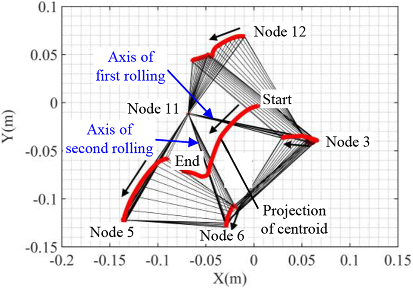
Projection of motion trajectories of centroid and typical nodes of gait TO–5→TC–5→TO–10. TC: closed triangle; TO: open triangle.

Analytical estimations

The traveling distances and locomotion directions of the gait primitives given in Table 4 are analytically estimated by geometrically unfolding the triangle faces, and the results are listed in Table 5. The corresponding numerical results using the relevant control strategies are also listed in Table 5 for comparison. Most of the errors between the numerical results and the analytical results are within 5%, indicating that the analytical method is acceptable in approximating the traveling distance and direction of a gait. The most likely reasons for the errors are the deformation of the tensegrity system and the moving of the rolling axis.

Table 5.

Comparison of traveling distance and locomotion direction.

No. of gait primitives	Traveling distance			Locomotion direction
No. of gait primitives	Analytical (cm)	Numerical (cm)	Errors (%)	Analytical (°)	Numerical (°)	Errors (%)
1	6.16	6.26	−1.60	212	216	−1.85
2	6.16	6.27	−1.75	332	336	−1.19
3	6.16	6.27	−1.75	92	96	−4.17
4	6.16	6.03	2.16	256	252	1.59
5	6.16	6.27	−1.75	32	36	−11.11
6	10.67	11.71	−8.88	286	292	−2.05
7	10.67	10.54	1.23	226	220	2.73
8	10.67	10.78	−1.02	62	69	−10.14
9	6.16	6.48	−4.94	212	214	−0.93
10	6.16	6.48	−4.94	332	334	−0.60
11	6.16	6.41	−3.90	92	94	−2.13
12	6.16	6.24	−1.28	256	254	0.79
13	6.16	6.27	−1.75	32	36	−11.11
14	10.67	10.48	1.81	62	62	0.00

Locomotion path based on idealized rolling gait primitives

A locomotion path can be quickly generated by combining the rolling gait primitives if the rolling gait primitives are idealized by their analytical counterparts.

To demonstrate the effectiveness of this simple path-generating strategy, a motion generated by rolling a full round on the spherical tensegrity is considered. In the full-round rolling, the touching-ground triangle of the tensegrity system starts from TC–6 (3, 7, 12) and finally comes back to this position by rolling past the triangles in the following sequence: TC–6 (3, 7, 12)→TO–5 (3, 11, 12)→TC–5 (3, 6, 11)→TO–10 (5, 6, 11)→TC–3 (2, 5, 11)→TO–1 (1, 2, 5)→TC–1 (1, 5, 10)→TO–3 (1, 9, 10)→TC–2 (1, 8, 9)→TO–11 (7, 8, 9)→TC–8 (4, 7, 9)→TO–7 (3, 4, 7)→TC–6 (3, 7, 12). The sequence of the touching-ground triangle shift is illustrated on the surface of the tensegrity in Figure 10(a) and unfolded on a plane in Figure 10(b). Note that the tensegrity system is not required to stop at each triangle in the sequence. Since there are double-rolling gaits, the tensegrity system can roll through a triangle in the sequence if a proper double-rolling gait is used. Two typical paths, one of them consisting of 12 single-rolling gaits and the other consisting of 2 single-rolling gaits and 5 double-rolling gaits, are shown in Figure 10(b). The displacements of the centroid geometrically determined based on Figure 10(b) are −0.543 and −0.243 m in x- and y-directions, respectively. The corresponding total traveling distance is 0.595 m.

Figure 10.

Locomotion path estimated by geometry: (a) touching-ground triangle sequence on the surface of tensegrity and (b) unfolded path.

Numerical simulation on the locomotion path consisting of two single-rolling gaits and five double-rolling gaits is conducted by using an incremental DRM as mentioned above. The control strategies of the used gaits determined by the GA-based gait-generating method are listed in Table 6. The locomotion path obtained by the simulation is shown in Figure 11. It can be seen that the overall shape of the simulated path is similar to that of the analytical path (Figure 10(b)). The simulated displacements of the centroid are −0.556 and −0.242 m in x- and y-directions, respectively, and the simulated total traveling distance is 0.606 m. The errors between the numerical results and analytical results of the displacements in x- and y-directions and the total traveling distance are 2.3%, 0.4%, and 1.8%, respectively. As these errors are within 5%, the results can usually be deemed to be acceptable in engineering applications. It is worth noting that a more elaborate approach for path planning of rolling locomotive spherical tensegrity systems based on the combination of rolling gait primitives has been developed in a previous study,⁷ and the work presented here supports the basic assumption adopted in this previous study.⁷

Table 6.

Rolling gaits and corresponding control strategies for numerical simulation on motion path.

Rolling gaits	Actuation length (cm)
Rolling gaits	1	2	3	4	5	6
TC–6→TO–5	−4.39	5.20	—	—	—	—
TO–5→TC–5→TO–10	5.30	−4.70	5.30	−4.70	—	—
TO–10→TC–3→TO–1	−4.70	5.30	−4.70	—	—	5.30
TO–1→TC–1→TO–3	—	−4.70	5.30	—	5.30	−4.70
TO–3→TC–2→TO–11	—	—	−4.70	5.30	−4.70	5.30
TO–11→TC–8→TO–7	5.30	—	—	−4.70	5.30	−4.70
TO–7→TC–6	—	—	—	5.30	—	—

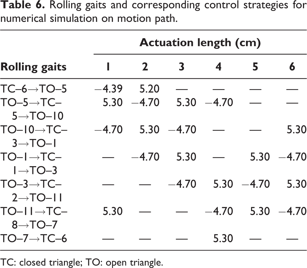
TC: closed triangle; TO: open triangle.

Figure 11.

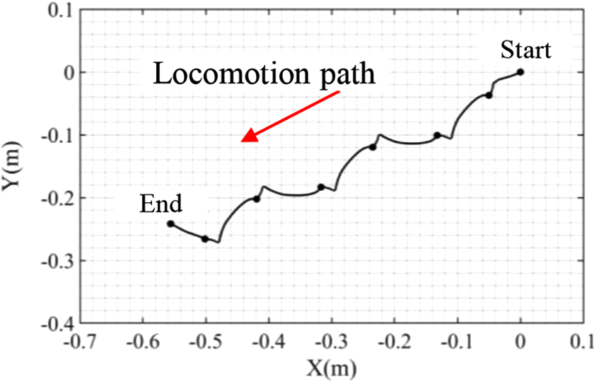
Locomotion path obtained by simulation.

Experiments

Physical prototype

A physical prototype of a strut-actuated six-strut tensegrity robot based on the configuration detailed in the “Strut-actuated six-strut spherical tensegrity” section was manufactured, as shown in Figure 12. The properties of the members used in the prototype are identical to those given in Table 2. Six servo linear actuators are used as active struts, and 24 springs are used as tendons. The servo linear actuators have an inextensible length of 15.6 cm and an extensible length of 10.0 cm. At their basic states, they extend to 20 cm to prestress the system. The telescopic rate of the actuators is 5 mm/s. In the center of the prototype system, a control box consisting of a Bluetooth communication module, a servo control module, and a lithium battery is attached to the nodes with 24 springs the same as those used for tendons. The weight of the control box is 151.6 g, and the total weight of the prototype is 598.5 g. The prototype is wirelessly controlled through Bluetooth communication with a control program installed in a personal computer.

Figure 12.

Physical prototype of strut-actuated six-strut tensegrity robot.

Validation of rolling gaits

Tests on typical rolling gaits

Twenty typical rolling gaits selected from the pool of numerically feasible rolling gaits generated by the computations performed in the “Rolling gaits” section are tested experimentally. Nine of these rolling gaits start with a TC state and end with a TO state, and the rest start with a TO state and end with a TC state. The corresponding control strategies of the tested gaits and their experimental results are given in Table 7, which shows that 19 of the 20 tested gaits are realized by the physical prototype.

Table 7.

Tested gaits and test results.

Initial state	Gait No.	Gait mode	Actuation length (cm)						Feasibility
Initial state	Gait No.	Gait mode	1	2	3	4	5	6	Feasibility
TC	1	TC–6→TO–5	−4.39	5.20	—	—	—	—	Yes
	2	TC–6→TO–7	5.00	—	−4.10	—	—	—	Yes
	3	TC–6→TO–12	—	−4.70	4.80	—	—	—	No
	4	TC–6→TO–5	−4.50	5.00	5.00	—	—	—	Yes
	5	TC–6→TO–12	−4.70	−4.70	5.30	—	−4.70	—	Yes
	6	TC–6→TO–7	5.00	4.90	−4.40	0.10	—	—	Yes
	7	TC–6→TO–12	5.00	−4.60	4.60	5.00	—	—	Yes
	8	TC–6→TO–5	−4.70	5.00	−3.30	—	—	—	Yes
	9	TC–6→TO–7	4.60	3.60	−4.50	—	0.20	−1.50	Yes
TO	10	TO–5→TC–5	5.00	—	—	—	—	—	Yes
	11	TO–5→TC–6	—	—	—	—	—	5.00	Yes
	12	TO–5→TC–5	5.00	2.00	—	—	—	—	Yes
	13	TO–5→TC–6	5.00	—	—	—	—	4.90	Yes
	14	TO–5→TC–5	5.00	3.40	−4.60	—	—	—	Yes
	15	TO–5→TC–6	−2.40	3.80	—	—	—	5.00	Yes
	16	TO–5→TC–5	5.00	2.40	−4.50	1.60	—	—	Yes
	17	TO–5→TC–6	3.50	1.50	−4.70	—	—	5.00	Yes
	18	TO–5→TC–5	5.00	2.30	−3.70	0.20	−2.70	—	Yes
	19	TO–5→TC–6	3.30	1.70	−4.60	2.60	—	5.00	Yes
	20	TO–5→TC–5	5.00	3.00	−4.70	2.30	5.00	2.10	Yes

TC: closed triangle; TO: open triangle.

Considering that the numerical model of the tensegrity robot is an idealized model that does not consider many details of the physical system, such as the configuration of the connections or the fabrication error, the experimental results indicate that the gait-generating approach used in this study is generally effective and has considerable robustness. The difference between the numerical model and the physical prototype can be seen in the inconsistency in the positions of touching-ground nodes and the deviation of locomotion directions. To reduce the effect of the uncertainties of connections and fabrication error, more elaborate physical prototypes will be produced for future studies.

Observations of rolling axes and traveling directions

Rolling around both fixed and moving axes in the experiments is observed. Rolling gait 1 (TC–6→TO–5) in Table 7 is taken as an example of rolling around a fixed axis (Figure 13(a)), and rolling gait 5 (TC–6→TO–12) is taken as an example of rolling around a moving axis (Figure 13(b)). In Figure 13, the projections of the centroids of the touching-ground triangles at the initial and final states are denoted as A′ and B′, respectively. The numerical traveling distance and direction of rolling gait 1 are 7.08 cm and 216°, respectively, and the numerical traveling distance and direction of rolling gait 5 are 7.15 cm and 100°, respectively.

Figure 13.

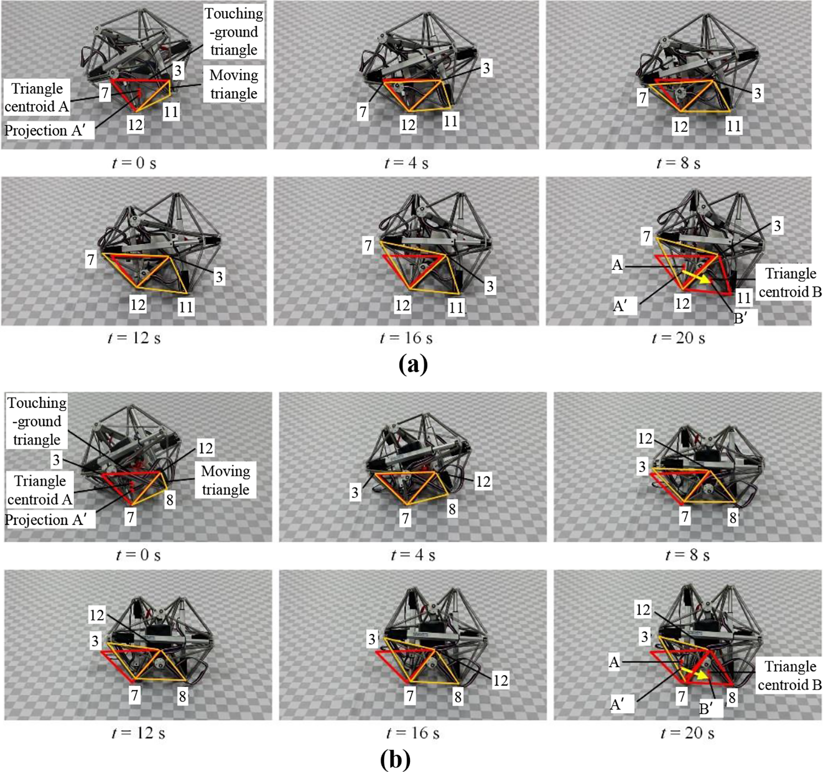
Experimental observation on rolling axes and traveling directions: (a) rolling around fixed axis and (b) rolling around moving axis.

In rolling gait 1 (TC–6→TO–5), the initial and final touching-ground triangles are TC–6 (3, 7, 12) and TO–5 (3, 11, 12), respectively. As shown in Figure 13(a), the system rolls around the tendon connecting nodes 12 and 3, which keep in contact with the ground and show no notable movement throughout the rolling process. Meanwhile, node 7 leaves the ground, whereas node 11 touches the ground. The traveling distance A′B′ is 7.75 cm, and the traveling direction is 206°. The relative errors of the traveling distance and direction between the experimental results and numerical results are 9.5% and 4.6%, respectively. In rolling gait 5 (TC–6→TO–12), the initial and final touching-ground triangles are TC–6 and TO–12, respectively. As shown in Figure 13(b), the system rolls around the tendon connecting nodes 7 and 12. Notable movement of node 7 can be observed at and after t = 8 s, whereas node 12 remains static. As a result, the rolling axis, that is, the tendon connecting nodes 7 and 12, rotates around node 12 by a certain degree on the ground. After the gait, node 3 leaves the ground, whereas node 8 comes in contact with the ground. The traveling distance A′B′ is again 7.75 cm, and the traveling direction is 86°. The relative errors of the traveling distance and direction between the experimental results and numerical results are 8.4% and 14.0%, respectively.

Validation of locomotion path

The gaits listed in Table 6 are applied to the physical prototype to validate the simple path-generating strategy. The motion process of the prototype in the experiment is shown in Figure 14. The locomotion paths obtained by the experiment and by using the simple strategy are illustrated in Figure 15. This shows that the error between the two paths increases as the number of gaits increases. The total traveling distances in the experimental path and the analytical path are 71.4 and 68.6 cm, respectively, and the error between the experimental and analytical traveling distances is 3.9%. The final displacements of the locomotive tensegrity in x- and y-directions in the experiment are −61.3 and −36.6 cm, respectively, whereas the counterparts determined by the simple strategy are −62.9 and −27.4 cm, respectively. The experimental displacement in the y-direction is significantly greater than the analytical one, resulting in a medium deviation in the traveling direction. These observations indicate that the unavoidable errors between the analytical rolling gaits used in the simple strategy and the real gaits deployed by the prototype cumulate as the number of gaits increases, especially for the traveling direction.

Figure 14.

Motion path of locomotive tensegrity.

Figure 15.

Locomotion paths determined by experiment and by analytical method.

Conclusions

In this study, a mathematical model based on combinatorial optimization and a method incorporating a GA with a DRM is presented to generate rolling gaits for a strut-actuated six-strut spherical tensegrity. Various rolling gaits using different numbers of active struts are identified and examined. A simple path-generating strategy based on analytical rolling gaits with fixed rolling axes is proposed. A physical prototype of the strut-actuated six-strut spherical tensegrity is manufactured, and experiments conducted.

From the results of simulation and experiments, the following observations can be made:

In most primitives, the tensegrity rolls once from one triangle to an adjacent triangle. In others, the tensegrity rolls twice from one triangle to an adjacent triangle, and the rolling axis may be fixed or moving.

The rolling gaits generated by the numerical approach and the simple path-generating strategy are conceptually verified by the experiments. Although some nonignorable errors between the simulated results and the experimental results are observed, they can be explained by the unavoidable difference between the numerical model of the locomotive tensegrity and the corresponding physical prototype.

The analytical model assumes the outside surface of the tensegrity to be an idealized and rigid icosahedron and does not consider the details of the physical system such as the configuration of the connections or the fabrication error and the deformation of the system during the rolling motion. These prerequisites lead to the inconsistency in the positions of touching-ground nodes and the deviation of locomotion directions. Using a more elaborate physical prototype which reduces the effect of the uncertainties of connections and fabrication error and an improved analytical model which takes the deformation of the system into account are believed to be able to reduce the errors between the analytical solutions and experimental results.

Footnotes

Declaration of conflicting interests

The author(s) declared no potential conflicts of interest with respect to the research, authorship, and/or publication of this article.

Funding

The author(s) disclosed receipt of the following financial support for the research, authorship, and/or publication of this article: This work was supported by the National Key Research and Development Program of China (Grant No. 2016YFC0800200); the Natural Science Foundation of Zhejiang Province (Grant Nos. LR17E080001 and Y18F030012), and the National Natural Science Foundation of China (Grant Nos. 51778568 and 51908492).

ORCID iDs

Meijia Wang

Xian Xu

References

Pugh

. An introduction to tensegrity. Berkeley, CA: University of California Press, 1976.

Sabouni-Zawadzka

Gilewski

. Inherent properties of smart tensegrity structures. Appl Sci 2018; 8: 787.

Peng

Kan

. A novel distributed model predictive control method based on a substructuring technique for smart tensegrity structure vibrations. J Sound Vib 2020; 471: 115171.

Sychterz

Smith

. Damage mitigation of near-full-scale deployable tensegrity structure through behavior biomimetics. J Struct Eng 2020; 146: 4019181.

Pizzigoni

Micheletti

Ruscica

, et al. A new T4 configuration for a deployable tensegrity pavilion. In: Proceedings of IASS annual symposia, Barcelona, Spain, 7–10 October 2019, pp. 1–6. International Association for Shell and Spatial Structures (IASS).

Rieffel

Mouret

. Adaptive and resilient soft tensegrity robots. Soft Robot 2018; 5: 318–329.

Luo

. Path planning for rolling locomotion of polyhedral tensegrity robots based on dijkstra algorithm. J Int Assoc Shell Spat Struct 2019; 60: 273–286.

Carreño

Post

. Design of a novel wheeled tensegrity robot: a comparison of tensegrity concepts and a prototype for travelling air ducts. Robot Biomimet 2018; 5: 1.

Mirletz

Park

Flemons

, et al. Design and control of modular spine-like tensegrity structures. In: Proceedings of the 6th world conference of the international association for structural control and monitoring (6WCSCM), Barcelona, Spain, July 2014.

10.

Kaufhold

Schale

Böhm

, et al. Indoor locomotion experiments of a spherical mobile robot based on a tensegrity structure with curved compressed members. In: 2017 IEEE international conference on advanced intelligent mechatronics (AIM), Munich, Germany, 3–7 July 2017, pp. 523–528. IEEE.

11.

Orki

Shai

Ayali

, et al. A model of caterpillar locomotion based on assur tensegrity structures. In: ASME 2011 international design engineering technical conferences and computers and information in engineering conference, Washington, DC, 28–31 August 2011, pp. 739–745. American Society of Mechanical Engineers.

12.

Bliss

Iwasaki

Bart-Smith

. Central pattern generator control of a tensegrity swimmer. IEEE/ASME Trans Mech 2012; 18: 586–597.

13.

Friesen

Pogue

Bewley

, et al. DuCTT: a tensegrity robot for exploring duct systems. In: 2014 IEEE international conference on robotics and automation (ICRA), Hong Kong, China, 31 May–7 June 2014, pp. 4222–4228. IEEE.

14.

Friesen

Glick

Fanton

, et al. The second generation prototype of a duct climbing tensegrity robot, DuCTTv2. In: 2016 IEEE international conference on robotics and automation (ICRA), Stockholm, Sweden, 16–21 May 2016, pp. 2123–2128. IEEE.

15.

Tietz

Carnahan

Bachmann

, et al. Tetraspine: robust terrain handling on a tensegrity robot using central pattern generators. In: 2013 IEEE/ASME international conference on advanced intelligent mechatronics, Wollongong, NSW, Australia, 9–12 July 2013, pp. 261–267. IEEE.

16.

Shibata

Saijyo

Hirai

. Crawling by body deformation of tensegrity structure robots. In: 2009 IEEE international conference on robotics and automation, Kobe, Japan, 12–17 May 2009, pp. 4375–4380. IEEE.

17.

Koizumi

Shibata

Hirai

. Rolling tensegrity driven by pneumatic soft actuators. In: 2012 IEEE international conference on robotics and automation, Saint Paul, MN, USA, 14–18 May 2012, pp. 1988–1993. IEEE.

18.

Kim

. On the locomotion of spherical tensegrity robots, Berkeley: University of California, 2016.

19.

Khazanov

Humphreys

Keat

, et al. Exploiting dynamical complexity in a physical tensegrity robot to achieve locomotion. In: Artificial life conference proceedings 13, September 2013, pp. 965–972. Cambridge, MA: MIT Press.

20.

Agogino

SunSpiral

Atkinson

. Super ball bot-structures for planetary landing and exploration—phase 1, Final report, Technical report, NASA Innovative Advanced Concepts (NIAC) Program, 2013.

21.

Sun Spiral

Agogino

Atkinson

. Super ball bot-structures for planetary landing and exploration—phase 2, Final report, Technical report, NASA Innovative Advanced Concepts (NIAC) Program, 2015.

22.

Bruce

Sabelhaus

Chen

, et al. SUPERball: exploring tensegrities for planetary probes. In: 12th international symposium on artificial intelligence robotics and automation in space (i-SAIRAS), Montreal, Canada, 17–19 June, 2014, pp. 1–7, Longueuil: Canadian Space Agency.

23.

Bruce

. Design, building, testing, and control of SUPERball: a tensegrity robot to enable new forms of planetary exploration, Santa Cruz: University of California, 2016.

24.

Pellegrino

Calladine

. Matrix analysis of statically and kinematically indeterminate frameworks. Int J Solids Struct 1986; 22: 409–428.

25.

Luo

. Collision-free shape control of a plane tensegrity structure using an incremental dynamic relaxation method and a trial-and-error process. Proc Instit Mech Eng Part G J Aerosp Eng 2013; 227: 266–272.

26.

Sun

Luo

, et al. Collision-free path planning of tensegrity structures. J Struct Eng 2014; 140: 4013084.

27.

Reddy

JN.

The penalty function method in mechanics—a review of recent advances. In: Penalty-finite element methods in mechanics; Proceedings of the winter annual meeting, Phoenix, AZ, 14–19 November 1982 (A83-28851 12–31). New York, NY: American Society of Mechanical Engineers, 1982, pp. 1–20.

28.

Koza

. Genetic programming II. Cambridge, MA: MIT Press, 1994.

29.

Van Laarhoven

Aarts

. Simulated annealing: theory and applications. Berlin: Springer, 1987, pp. 7–15.

30.

Paul

Valero-Cuevas

Lipson

. Design and control of tensegrity robots for locomotion. IEEE Trans Robot 2006; 22: 944–957.

31.

Chipperfield

Fleming

Pohlheim

. Genetic algorithm toolbox: for use with MATLAB; user’s guide (version 1.2). Sheffield: University of Sheffield, Department of Automatic Control and Systems Engineering, 1994.

Rolling gaits of a strut-actuated six-strut spherical tensegrity

Abstract

Keywords

Introduction

Generating of rolling gaits

Mathematical model

Numerical method

Strut-actuated six-strut spherical tensegrity

Rolling gaits

Summary of gait-generating results

Rolling gait primitives

Rolling axis

Analytical estimations

Locomotion path based on idealized rolling gait primitives

Experiments

Physical prototype

Validation of rolling gaits

Tests on typical rolling gaits

Observations of rolling axes and traveling directions

Validation of locomotion path

Conclusions

Footnotes

Declaration of conflicting interests

Funding

ORCID iDs

References