Sage Journals: Discover world-class research

Abstract

To address the Jacobian matrix approximation error, which usually exists in the iterative solving process of the classic singular robust inverse method, the correction coefficient α is introduced, and the improved singular robust inverse method is the result. On this basis, the constant improved singular robust method and the intelligent improved singular robust inverse method are proposed. In addition, a new scheme, combining particle swarm optimization and artificial neural network training, is applied to obtain real-time parameters. The stability of the proposed methods is verified according to the Lyapunov stability criteria, and the effectiveness is verified in the application examples of spatial linear and curve trajectories with a seven-axis manipulator. The simulation results show that the improved singular robust inverse method has better optimization performance and stability. In the allowable range, the terminal error is smallest, and there is no lasting oscillation or large amplitude. The least singular value is largest, and the joint angular velocity is smallest, exactly as expected. The derivative of the Lyapunov function is negative definite. Comparing the two extended methods, the constant improved singular robust method performs better in terms of joint angular velocity and least singular value optimization, and the intelligent improved singular robust inverse method can achieve a smaller terminal error. There is little difference between their overall optimization effects. However, the adaptability of the real-time parameters makes the intelligent improved singular robust inverse method the first choice for kinematic control of redundant serial manipulators.

Keywords

Improved singular robust inverse method intelligent algorithm redundant manipulators inverse kinematics

Introduction

Kinematics is the basis of manipulator control technology, which focuses on inverse kinematics solutions.^1

–5 However, due to the high nonlinearity of redundant manipulators, it is quite difficult to obtain a suitable solution. The classic method is used to obtain the pseudoinverse solutions of various target functions.^6
–8 Many related research papers have been published.^{1,2,6,9
–11}

The singular value decomposition generalized inverse method (SGIM) is a classical and common scheme to obtain inverse kinematics solutions for redundant manipulators, which provides a well-defined Jacobian generalized inverse matrix by singular value decomposition.^5,9,12 Although the least norm under least-squares solutions can be easily obtained by the SGIM,^9,12 the practicality of the solution will suffer, because the norm of the angular velocity tends to infinity when the least singular value approaches zero. Therefore, another new method, the singular robust inverse method (SRIM), has been proposed.^{6
–8,10,11,13

–17} The SRIM introduces the damping coefficient λ to the SGIM to solve the singular problem caused by the small scale of the least singular value, and it reconstructs a new optimization target function. However, the optimization effect depends largely on the value of the damping coefficient λ. So far, scholars have proposed various definitions of λ. Wampler¹⁰ suggested that the damping coefficient λ was a constant. Kelmar and Khosla,¹³ Chan and Lawrence,¹⁴ Nakamura and Hanafusa,⁷ and others^6,15 have proposed definitions of the piecewise functions for λ. In addition, intelligent algorithms^16,18 have also been used to find better damping coefficients in recent years. All these schemes can treat λ as a function of singular values of the Jacobian matrix, which is obviously nonlinear.

Artificial neural networks (ANNs) and particle swarm optimization (PSO) are widely used in solving inverse kinematics of manipulators.^{18

–25} ANNs adopt the parallel computing method, which is efficient, fast, and suitable for dealing with the nonlinear relationships among a large number of data.²⁰ However, the disadvantage is also obvious: It is essential to prepare the original data set for training. The acquisition of data usually relies on data recording of motion history,¹⁹ data collection with trial-and-error methods,¹⁸ and formula deduction under restricted conditions.²¹ The data obtained by these methods cannot guarantee sufficient optimization.

On the other hand, there are also some problems in solving the inverse kinematics of a manipulator using PSO. Considering iteration with a wide range and a large number of random seed particles, although there is a high probability of obtaining globally optimal data, it consumes many computing resources, which is not suitable for online computing. To solve this problem, Dereli and Köker,²³ Shen et al.,²⁴ and other scholars²⁵ adopt approaches such as limiting an articular angle independent variable or narrowing the overall initial search range to improve the speed of calculation. Clearly, these methods make PSO unable to obtain the optimal solutions.

Combining the advantages of the above two intelligent algorithms and utilizing PSO to obtain the optimal data set of a wide range and a large number of random seed particles off-line while training the data with an ANN. The obtained training model not only realizes the optimization as much as possible but also meets the real-time prediction of the damping factors. And it is a feasible scheme.

Compared with the SGIM, the SRIM has achieved better results in solving the inverse kinematics problem of redundant manipulators; however, there are also some shortcomings, as follows:

(i) In the iterative solution of inverse kinematics, to obtain the joint angle variable Δθ from t_k to t_k ₊₁, the Jacobian matrix is usually considered to be unchanged, and the value at t_k is used as an approximation substitution value, as follows

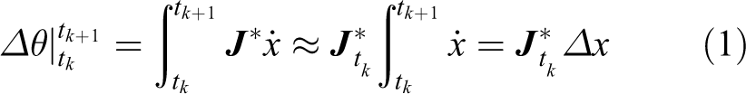
Δ θ |_{t_{k}}^{t_{k + 1}} = \int_{t_{k}}^{t_{k + 1}} J^{*} \dot{x} \approx J_{t_{​_{k}}}^{*} \int_{t_{k}}^{t_{k + 1}} \dot{x} = J_{t_{​_{k}}}^{*} Δ x

Once the manipulator passes a singular point between t_k and t_k ₊₁, the singular values of the Jacobian matrix will change significantly, and the approximation will produce a larger terminal error. Employing a smaller sampling interval can eliminate the error, but more computing resources will be consumed. Obviously, neither the SRIM nor the SGIM considers the effect of approximation.

(ii) There are many factors affecting the values of the damping coefficient, such as operability, the least singular value, and the matrix condition number. However, in the final analysis, the damping coefficient can be regarded as a mapping function of Jacobian matrix singular values that is time-varying and nonlinear. Classical constant coefficients and traditional damping functions cannot reflect the highly nonlinear relationship and struggle to provide real-time optimal damping parameters.

To overcome the defects of the SRIM, a pre-factor α is employed to eliminate the error caused by the approximation of the Jacobian matrix. An improved singular robust inverse method (ISRIM) with double coefficients α–λ is formed. The influences of the introduction of α on the terminal error and joint angular velocity are analyzed, and the Lyapunov function is also introduced to analyze the stability of the process. On this basis, the corresponding data set of damping factors and singular values of the Jacobian matrix are obtained by PSO and further trained by an ANN to obtain the simulated Simulink fitting model; the obtained model is used to predict the α–λ factors, which are essential for the real-time optimization of inverse kinematics. In addition, the simulations of the example confirmed the effectiveness of the proposed methods.

The double coefficients introduced in the ISRIM provide more adjustment measures for obtaining inverse kinematics solutions. The real-time prediction of the coefficients by PSO-ANN supports an innovative scheme for the online solutions of inverse kinematics. The numerical method is used in the solving process, and it is more easily extended to multi-axis redundant manipulators. The proposed method has made an exploratory study on the inverse kinematics solution of redundant manipulators, which lays a theoretical foundation for the precise control and wider use of series redundant manipulators.

The present work employs a pre-factor α to overcome the mentioned shortcomings of the SRIM and introduces intelligent PSO-ANN algorithms for real-time inverse kinematics solutions. The basic preparation and the SGIM and SRIM models are presented in the second section. The new methodology, the ISRIM, is illustrated in the third section. The modified methods are applied to a seven-axis manipulator for validation and comparison in the fourth section. The article ends with the conclusion in the final section.

Preliminaries

The mapping between the joint space and operation space is the main research of kinematics.³ It is highly nonlinear for redundant manipulators. Therefore, it must be linearized to meet the motion control requirements.

The classical linearization method is to build the equation using the Jacobian matrix.²⁶ If it is divided by time, we can obtain the corresponding speed linear relationship as follows

{\dot{x}}_{t} = J (θ_{t}) {\dot{θ}}_{t}

where J(θ_t ) is an m × n partial derivative Jacobian matrix.

The differential form of equation (2) can be expressed as

Δ x = J (θ) Δ θ

Then, we have

Δ θ = J {(θ)}^{*} Δ x

where J (θ)* (abbreviated J *) is the inverse of the corresponding Jacobian matrix J (θ) (abbreviated J ).

Singular value decomposition generalized inverse method

J is a rectangular matrix whose inversion is different from that of the general square matrix. In 1955, based on the research of Moore,²⁷ the British mathematician Penrose²⁸ defined the generalized matrix inverse, which is known as the M-P generalized inverse (or “+” inverse). The M-P inverse can provide all matrices’ inversions, including that of the rectangle matrix, and it is unique; this result can be obtained by singular value decomposition.⁹

After singular value decomposition, the matrix J can be expressed as

J = U Σ V^{T} = \sum_{i = 1}^{r} u_{i} σ_{i} v_{i}^{T}

Furthermore, the corresponding inverse matrix J * can be written as

J^{*} = J^{+} = V Σ^{+} U^{T} = \sum_{i = 1}^{r} v_{i} σ_{i}^{+} u_{i}^{T}

where U is an m × m order orthogonal matrix. V is an orthogonal matrix of order n × m. m is the row number of the Jacobian matrix and n is the column number. Σ = diag(σ ₁, σ ₂,…, σ_r ), and $Σ^{+} = diag (σ_{1}^{- 1}, σ_{2}^{- 1}, \dots, σ_{r}^{- 1})$ . Both of them are diagonal matrices. σ ₁, σ ₂, …, and σ_r are the singular values of the matrix J , and they are decreasing. r is the rank of J , where r ≤ m.

For a row full rank matrix, the optimization of formula (2) with the SGIM is the least-norm solution under the least-squares condition, which can be expressed as follows

\begin{array}{l} {\begin{matrix} min {‖ \dot{θ} ‖}_{2} \\ subject to min {‖ δ ‖}_{2} \end{matrix} \\ s.t. \dot{x} - J \dot{θ} = δ \end{array}

The least-norm solution norm and the least terminal error norm corresponding to equation (7) are

\begin{array}{l} ‖ \dot{θ} ‖_{2} = {‖J^{+} \dot{x}‖}_{2} = ‖ V Σ^{+} U^{T} \dot{x} ‖_{2} \\ = \sqrt{{\dot{x}}^{T} U {(Σ^{+})}^{2} U^{T} \dot{x}} \\ = \sqrt{\sum_{i = 1}^{m} \frac{χ_{i}^{2}}{σ_{i}^{2}}} \end{array}

{‖δ‖}_{2} = {‖ \dot{x} - J \dot{θ} ‖}_{2} = {‖\dot{x} - J J^{+} \dot{x}‖}_{2} = 0

where ${[χ_{1}, \dots χ_{m}]}^{T} = U^{T} \dot{x}$ . The other parameters are defined as above.

Singular robust inverse method

The SRIM, also known as the damped least-squares method,¹¹ improves the membership of the least norm and least squares in the optimization target in equation (7) so that it is a parallel relationship. It also employs a damping coefficient λ to balance them. Therefore, a new optimization target function $G {(\dot{θ})}_{λ}$ is proposed.

G {(\dot{θ})}_{λ} = {‖ \dot{x} - J \dot{θ} ‖}_{2} + λ {‖ \dot{θ} ‖}_{2}

Then, the optimization of the solution of formula (2) can be expressed as

\begin{array}{l} min_{\dot{θ}} ‖ \dot{x} - J \dot{θ} ‖_{2} + λ ‖ \dot{θ} ‖_{2} \\ s.t. \dot{x} - J \dot{θ} = δ \end{array}

The solution norm ${‖ {\dot{θ}}_{λ} ‖}_{2}$ and the terminal error norm ${‖δ_{λ}‖}_{2}$ with damping λ can be written as

\begin{array}{l} ‖ {\dot{θ}}_{λ} ‖_{2} = ‖ J_{λ}^{*} \dot{x} ‖_{2} = ‖ J^{T} {(J J^{T} + λ E)}^{- 1} \dot{x} ‖_{2} \\ = \sqrt{\sum_{i = 1}^{m} \frac{σ_{i}^{2} χ_{i}^{2}}{{(σ_{i}^{2} + λ)}^{2}}} \end{array}

\begin{array}{l} {‖δ_{λ}‖}_{2} = ‖ \dot{x} - J J_{λ}^{*} \dot{x} ‖_{2} = ‖ \dot{x} - J J^{T} {(J J^{T} + λ E)}^{- 1} \dot{x} ‖_{2} \\ = \sqrt{{\sum_{i=1}^{m} (\frac{λ}{σ_{i}^{2} + λ})}^{2} χ_{i}^{2}} \end{array}

where all of the parameters are as above.

New singularity-avoidance schemes

In the present work, based on the SRIM, we propose a new scheme, the ISRIM. The optimization of equation (2) in the ISRIM can be expressed as

\begin{array}{l} min_{\dot{θ}} ‖ \dot{x} - α J \dot{θ} ‖_{2}^{2} + ‖ λ \dot{θ} ‖_{2}^{2} \\ s.t. \dot{x} - J \dot{θ} = δ \end{array}

In equation (14), a pre-coefficient α is employed for the target function, whose purpose is to eliminate the terminal error caused by the approximation of the Jacobian matrix when the manipulator passes singular points. The optimization target function is reconstructed as

\begin{array}{l} G {(\dot{θ})}_{α λ} = ‖ \dot{x} - α J \dot{θ} ‖_{2}^{2} + ‖ λ \dot{θ} ‖_{2}^{2} \\ = [\begin{matrix} {(\dot{x} - α J \dot{θ})}^{T} & {\dot{θ}}^{T} \end{matrix}] [\begin{matrix} E_{m \times m} & 0 \\ 0 & λ^{2} I_{n} \end{matrix}] [\begin{matrix} \dot{x} - α J \dot{θ} \\ \dot{θ} \end{matrix}] \\ = {(\dot{θ} - {\dot{θ}}_{α λ})}^{T} (α^{2} J^{T} J + λ^{2} I_{n}) (\dot{θ} - {\dot{θ}}_{α λ}) + {\dot{x}}^{T} W_{α λ} \dot{x} \end{array}

In equation (15)

W_{α λ} = I_{m} - α J {(α^{2} J^{T} J + λ^{2} I_{n})}^{- 1} J^{T} α

Since α ² J ^T J + λ ² I_n is positive definite in formula (15), $G {(\dot{θ})}_{α λ}$ is a positive-definite quadratic form of $\dot{θ}$ , and has a minimum value only if $\dot{θ} = {\dot{θ}}_{α λ}$ . Then, the solution of formula (2) for the optimum configuration (14) is as follows

{\dot{θ}}_{α λ} = {(α^{2} J^{T} J + λ^{2} I_{n})}^{- 1} J^{T} α \dot{x}

The improved singular robust inverse of the Jacobian matrix corresponding to equation (17) is

J_{α λ}^{*} = {(α^{2} J^{T} J + λ^{2} I_{n})}^{- 1} J^{T} α

Furthermore, $J_{α λ}^{*}$ can be expressed as a simple calculation⁷ as follows

J_{α λ}^{*} = J^{T} α {(α^{2} J J^{T} + λ^{2} I_{m})}^{- 1}

Then, for the full-rank Jacobian matrix J , the least-norm solution norm ${‖ {\dot{θ}}_{α λ} ‖}_{2}$ and the least terminal error norm ${‖ {\dot{δ}}_{α λ} ‖}_{2}$ of ISRIM are

\begin{array}{l} ‖ {\dot{θ}}_{α λ} ‖_{2} = ‖ J_{α λ}^{*} \dot{x} ‖_{2} \\ = ‖ J^{T} α {(α^{2} J J^{T} + λ^{2} I_{m} ​^{m})}^{- 1} \dot{x} ‖_{2} \\ = \sqrt{\sum_{i = 1}^{m} \frac{α^{2} σ_{i}^{2}}{{(α^{2} σ_{i}^{2} + λ^{2})}^{2}} χ_{i}^{2}} \end{array}

\begin{array}{l} ‖ δ_{α λ} ‖_{2} = ‖ \dot{x} - J J_{α λ}^{*} \dot{x} ‖_{2} \\ = ‖ \dot{x} - J J^{T} α {(α^{2} J J^{T} + λ^{2} I_{m})}^{- 1} \dot{x} ‖_{2} \\ = \sqrt{{\sum_{i=1}^{m} (\frac{α^{2} σ_{i}^{2} - α σ_{i}^{2} + λ^{2}}{α^{2} σ_{i}^{2} + λ^{2}})}^{2} χ_{i}^{2}} \end{array}

During the tracking trajectory process, $\dot{θ}$ can be ultimately expressed as

\dot{θ} = {\dot{θ}}_{α λ} + {\dot{θ}}_{δ} = J_{α λ}^{*} {\dot{x}}_{d} + J_{α λ}^{*} δ_{α λ}

where ${\dot{x}}_{d}$ is the desired terminal velocity of the manipulator. $\dot{x}$ is the actual terminal velocity. $δ_{α λ}$ is the terminal position error.

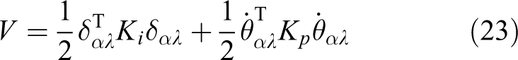
According to the stability criterion,^29

–34 the stability of the proposed method was analyzed and the Lyapunov function²⁹ was defined as

V = \frac{1}{2} δ_{α λ}^{T} K_{i} δ_{α λ} + \frac{1}{2} {\dot{θ}}_{α λ}^{T} K_{p} {\dot{θ}}_{α λ}

Then, we have

\begin{array}{l} \dot{V} = δ_{α λ}^{T} K_{i} {\dot{δ}}_{α λ} + {\dot{θ}}_{α λ}^{T} K_{p} {\ddot{θ}}_{α λ} \\ = δ_{α λ}^{T} K_{i} ({\dot{x}}_{d} - \dot{x}) + {\dot{θ}}_{α λ}^{T} K_{p} {\ddot{θ}}_{α λ} \\ = δ_{α λ}^{T} K_{i} {\dot{x}}_{d} - δ_{α λ}^{T} K_{i} J_{α λ} \dot{θ} + {\dot{θ}}_{α λ}^{T} K_{p} {\ddot{θ}}_{α λ} \\ = - δ_{α λ}^{T} K_{i} δ_{α λ} + {\dot{θ}}_{α λ}^{T} K_{p} {\ddot{θ}}_{α λ} \end{array}

where K_i and K_p are positive constant coefficients, and they are determined by the actual speed. From formula (23), V is always positive definite. $\dot{V}$ determines the stability of the proposed method whether it is positive or not. Obviously, we can satisfy the stability requirement of $\dot{V}$ being negative definite by appropriately selecting the values of parameters α and λ.

Taking α and λ as simple constants, the obtained solutions will maintain good coherence. However, the selection of α and λ requires multiple attempts. This method is called constant improved singular robust inverse method (CISRIM). To obtain better real-time parameters, intelligent algorithms can be used. It is convenient to refer to this method as the intelligent improved singular robust inverse method (IISRIM). According to the previous literatures,^{6
–8,10,13,14} we know that the values of the parameters α and λ, which satisfy the objective function formula (14), are functions of the singular values of the Jacobian matrix. However, it should be pointed out that the function is nonlinear and multivariable and suitable for adopting the PSO algorithm.^23
–25,35

The core algorithm of PSO relies on the updating of velocity v and position p_x . Assuming that the total number of particles is N and each particle is a D-dimensional variable, the classical update functions³⁵ for the position and velocity of the jth component of the ith particle can be expressed as

v_{i j} = w v_{i j} + c_{1} r_{1} (p_{b i j} - v_{i j}) + c_{2} r_{2} (p_{g i j} - v_{i j})

p_{x_{i j}} = p_{x_{i j}} + v_{i j}

where v is the speed of the particle. p_x is the displacement value of the particle. w is the inertia weight. c ₁ and c ₂ are acceleration constants. r ₁ and r ₂ are acceleration weight coefficients.

The objective function represents the optimization purpose of PSO. According to the previous solution and stability analysis, the goal of α and λ optimization can be set as

\begin{array}{l} min_{α, λ} {‖δ_{α λ}‖}_{2} + ‖ {\dot{θ}}_{α λ} ‖_{2} \\ s.t. - δ_{α λ}^{T} K_{i} δ_{α λ} + {\dot{θ}}_{α λ}^{T} K_{p} {\ddot{θ}}_{α λ} < 0 \end{array}

According to the literature^25,32 and actual needs, we set the parameters of the PSO algorithm as follows: The total number of particles N is 50.0. The dimension of the particle is 2.0. The acceleration constants c ₁ and c ₂ are 1.0 and 2.0, respectively. The acceleration weight coefficients r ₁ and r ₂ are random numbers between 0.0 and 1.0. It should be noted that both parameters α and λ are within the range 0–10 based on experience.

The flowchart for obtaining the Jacobian matrix singular values and the corresponding α and λ values satisfying equation (27) is shown in Figure 1.

Figure 1.

Flowchart of the PSO algorithm. PSO: particle swarm optimization.

The data set consists of singular values of the Jacobian matrix and the corresponding damping coefficients, which are acquired by the PSO method and should be fitted and trained by the ANN. According to the literature^18

–22 and simulation experiences, the design of the ANN is as follows: (1) To avoid “over-adaptation” of the training, the obtained Jacobian matrix singular value data set is normalized by the mapminmax function. (2) A back-propagation (BP) neural network is adopted. The input is six singular values of the Jacobian matrix, and it has six neurons. The output is the corresponding α and λ values, so there are two neurons. For one hidden layer, according to the test, when the number of neurons is 50, better optimization results can be obtained. (3) The Levenberg–Marquardt algorithm is adopted. The other main parameters are set as follows: The number of epochs is 1000, min_grad is 1e−07, mu is 0.001, and max_fail is 6.

The established fitting neural network structure is shown in Figure 2.

Figure 2.

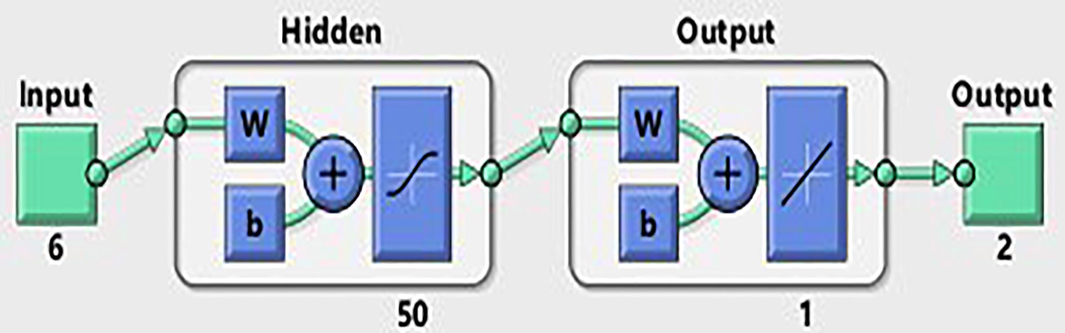
Structure of the established fitting neural network.

After training (Figure 3), it can be seen that the iterative process is completed after 13 iterations, and the obtained mean squared error is 1.3456e−11, which satisfies the requirements.

Figure 3.

Change of MSE with the epochs. MSE: mean squared error.

The training of the neural network and the simulation of the “Numerical simulation and analysis of results” section are implemented with the Neural Network Toolbox in MATLAB R2018b on a Lenovo T460 laptop computer with an Intel(R) Core(TM) i7-6500U CPU @ 2.50 GHz (4 CPUs), approximately 2.6 GHz.

The result of the ANN training is derived into the Simulink (R2019 of MATLAB) model and added in the overall Simulink model of inverse kinematics. Then, the parameter values of α and λ and the real-time inverse kinematics solutions can be obtained. The whole Simulink solving model is shown in Figure 4.

Figure 4.

Simulation model of tracking the spatial trajectory while incorporating the intelligent algorithm.

Numerical simulation and analysis of results

Taking the seven-axis manipulator “YL101” designed by the laboratory as the research object, the optimization of the CISRIM and IISRIM was studied, and the SGIM and SRIM were compared; these are well-known classic methods providing inverse kinematic solutions.

The structure of the manipulator “YL101” is shown in Figure 5, and its denavit-hartenberg (DH)³⁶ structural parameters are also listed in Table 1.

Figure 5.

Structural diagram of the “YL101” seven-axis manipulator.

Table 1.

DH structural parameters of the “YL101” manipulator.

θ	d (mm)	a (mm)	α (°)
θ ₁	105	0	90°
θ ₂	0	500	0
θ ₃	0	274	−90
θ ₄	0	198.5	90°
θ ₅	0	198.5	−90°
θ ₆	0	195	90°
θ ₇	236	0	0°

Example 1: Linear trajectory

The first simulation trajectory is the spatial line L_S , which extends from the initial point S_p (61.2 mm, −973.0 mm, 544.5 mm) to the end point E_p (807.9 mm, −334.3 mm, 730.5 mm), and the corresponding roll-pitch-yaw (RPY)³⁶ attitude angle from S_a (−146.1°, 5.0°, −3.9°) to E_a (−96.0°, 44.2°, −0.8°). The terminal accuracy error is less than 0.5 mm.

Due to the error accuracy requirements, the step size is set to be 0.05 mm. There are no parameters set for the SGIM. The damping coefficient λ of the SRIM is set as λ = λ ₀||δ||². According to the recommendation of Chan and Lawrence,¹⁴ the best results of the SRIM can be achieved when λ ₀ = 1.8. In the proposed CISRIM, after many attempts, better data can be obtained with α = 2.1 and λ = 0.35. In contrast to the CISRIM, another proposed method, the IISRIM, is an intelligent algorithm that does not require parameter settings. In addition, the time of a single step is set as 0.002 s. K_i and K_P are 1.0 and 0.008, respectively. The simulation results of the four methods are shown in Figures 6 to 11.

Figure 6.
Terminal errors of different optimizing methods in the spatial linear trajectory (“a” shows the singular points in an enlarged area).

Figure 7.
Lyapunov objective function derivative value $\dot{V}$ with different optimizing methods in the spatial linear trajectory (“b” shows $\dot{V}$ in an enlarged area).

Figure 8.
Joint angular velocity norm of different optimizing methods in a spatial linear trajectory.

Figure 9.
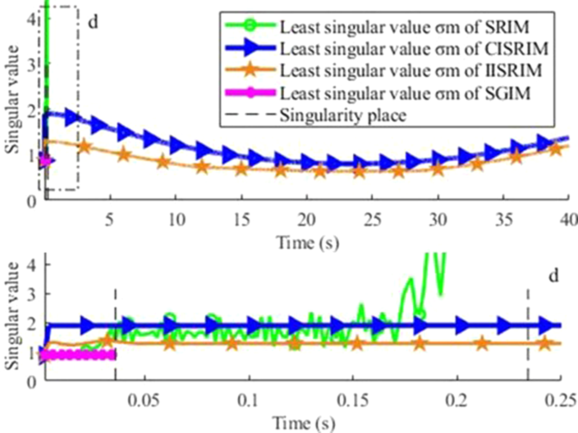
Least singular value of different optimizing methods in a spatial linear trajectory.

Figure 10.
Position and posture changes of the IISRIM in a spatial linear trajectory. IISRIM: intelligent improved singular robust inverse method.

Figure 11.
Joint angle values of the IISRIM in a spatial linear trajectory. IISRIM: intelligent improved singular robust inverse method.

The terminal errors of the four different methods are compared in Figure 6. When approaching the first singularity point, the SGIM results begin to oscillate and diverge. Due to the employed damping factor λ, the SRIM finds the solution of the first singular point, but the terminal error is large, and it always oscillates in subsequent iterations. When approaching the second singularity, the tolerance is also exceeded. The performance of the CISRIM and IISRIM based on the SRIM are much better, and both successfully obtain the inverse motion solutions. In contrast, the IISRIM’s solution converges quickly, with smaller amplitudes and fewer terminal errors, but appears to be slightly oscillating. The solutions of the CISRIM have better coherence, and no fluctuation appears after stabilization.

The prerequisite for obtaining correct solutions is solving stability. Figure 7 shows the Lyapunov objective function derivative value $\dot{V}$ with different optimizing methods. $\dot{V}$ should be negative, which is necessary for stability. Clearly, during the solving process, the $\dot{V}$ functions of the SGIM and SRIM produce positive values in turn. In contrast, the proposed CISRIM and IISRIM always have a negative $\dot{V}$ and satisfy the stability requirement.

In addition to the terminal error, the norm of joint angular velocity is also an indicator of manipulators, which should be small enough to be practical. As seen from Figure 8, the joint angular velocity of the SGIM is increasing and rapidly diverging, breaking the allowable value. Although the SRIM obtains a finite velocity value at the first singularity, it continues to oscillate and diverges at the second singularity place. In comparison, the angular velocities of the CISRIM and IISRIM are almost completely combined and maintain low values. However, it should be noted that the IISRIM’s angular velocity value has a small fluctuation, whose amplitude is not too large to affect the solving process.

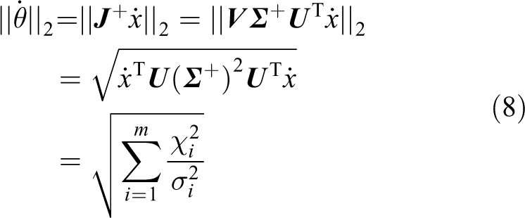
Equation (8) indicates that smaller singularity values will lead to a larger joint angular velocity and less flexibility of the manipulator. Therefore, to obtain stable solutions, the least singular value σ_m of the Jacobian matrix should be as large as possible. The σ_m of the SGIM is the smallest. The SRIM’s σ_m continues to oscillate and diverge. Only the least singular values σ_m of the Jacobian matrix obtained by the CISRIM and IISRIM are continuously stable. The CISRIM performs better for larger σ_m values.

In terms of the terminal error, joint angular velocity, and least singular value, the two new methods, the CISRIM and IISRIM, have their own advantages and disadvantages. However, it should be pointed out that the parameters of the CISRIM are obtained by the trial process. In contrast, the IISRIM without adjusted parameters is more suitable for engineering practice. Figures 10 and 11 show the track of the manipulator and the trend of the joint angle as well as the track of the spatial line L_S by the IISRIM. There are no drastic changes, and the IISRIM can meet the actual operational requirements.

In the process of tracking the spatial linear trajectory L_S , the ISRIM has a better optimization effect than the traditional SGIM and SRIM, with a more stable solution, smaller terminal error, smaller joint angular velocity, and larger least singular value. The CISRIM and IISRIM, extended on the basis of the ISRIM, have their own advantages. The CISRIM performs better in optimizing the least singular value σ_m . The IISRIM performs well in reducing terminal error, and there is little difference in terms of joint speed. In addition, it should be emphasized that the IISRIM does not have to adjust parameters. Once the training is completed, it can easily track the spatial trajectory, while the CISRIM does not.

Example 2: Curve trajectory

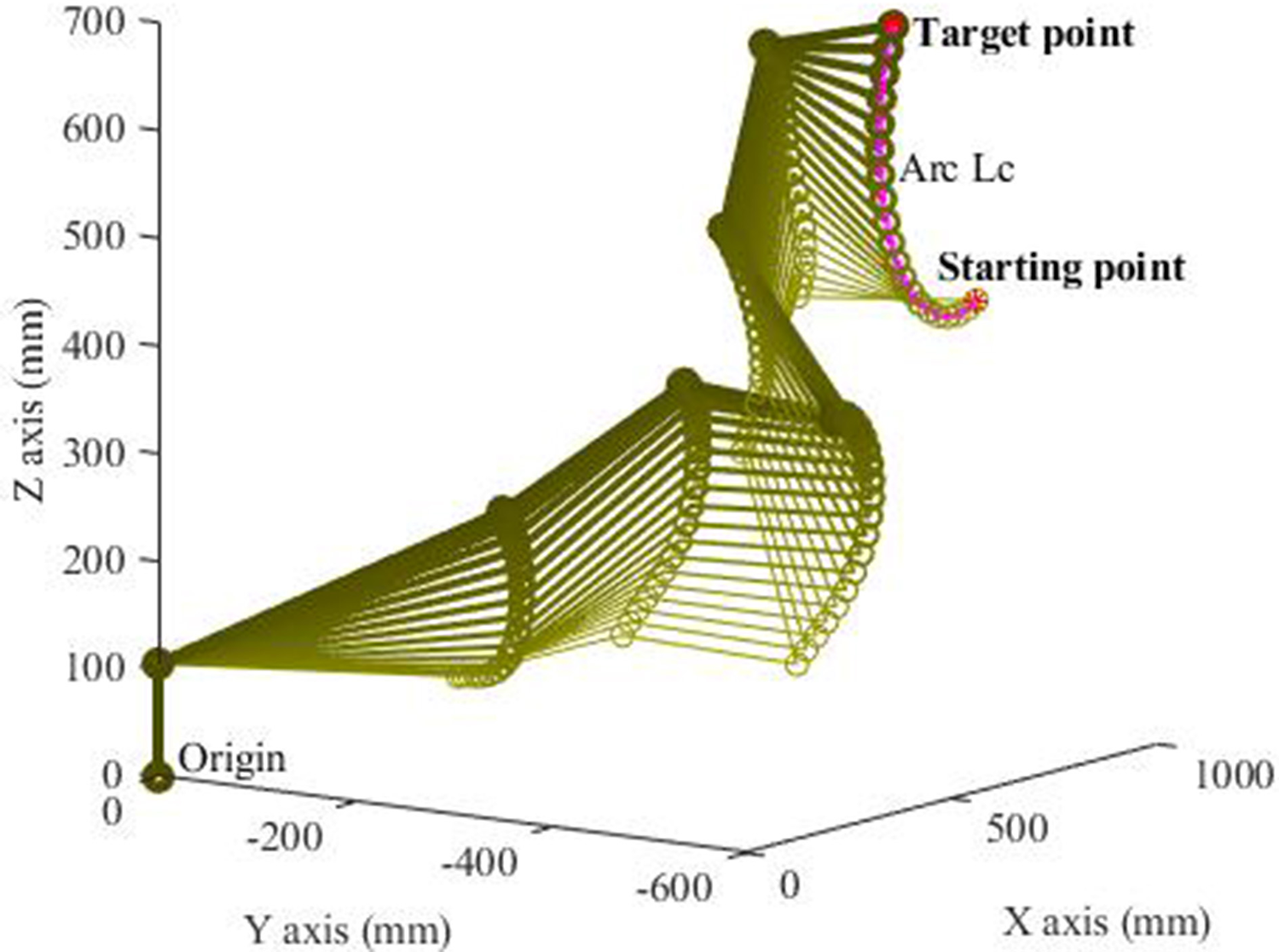
The second simulation trajectory is the spatial arc L_C , which extends from the initial point S_p (776.8 mm, −509.1 mm, 423.6 mm) to the end point E_p (574.2 mm, −509.0 mm, 698.6 mm), and the corresponding RPY attitude angle from S_a (−111.1°, 169.2°, −142.8°) to E_a (−125.5°, 161.1°, −103.8°). The terminal accuracy error is also less than 0.5 mm, with a circle center of O_c (721.2, −509.1, 594.8) and a normal vector of n_c (0, −1, 0).

The arclength step size is also set to be 0.05 mm. The parameter λ ₀ of the SRIM is set to be 0.1. The parameters of the CISRIM are α = 3.2 and λ = 3.0, and the other parameters are the same as in Example 1. The simulation results are shown in Figures 12 to 17.

Figure 12.
Terminal errors of different optimizing methods in a spatial arc trajectory (“e” shows the singular points in an enlarged area).

Figure 13.
Lyapunov function derivative value $\dot{V}$ with different optimizing methods in a spatial arc trajectory (“f” shows $\dot{V}$ in an enlarged area).

Figure 14.
Joint angular velocity norm of different optimizing methods in a spatial arc trajectory (“g” shows the singular points in an enlarged area).

Figure 15.
Least singular value of different optimizing methods in a spatial arc trajectory (“h” shows the singular points in an enlarged area).

Figure 16.
Position and posture changes of the IISRIM in a spatial arc trajectory. IISRIM: intelligent improved singular robust inverse method.

Figure 17.
Joint angle values of the IISRIM in a spatial arc trajectory. IISRIM: intelligent improved singular robust inverse method.

In addition to straight lines, tracking a curving trajectory is also a common basic task. As shown in Figure 12, similar to the straight line, only the proposed CISRIM and IISRIM can correctly solve the trajectory of the entire curve L_C . Comparing the two methods, the IISRIM can obviously obtain smaller terminal error solutions. The $\dot{V}$ values of the two methods are shown in Figure 13. Both of them are not positive and satisfy the stability requirement.

In addition, the changes in the joint angular velocity and the least singular value of different optimization methods are compared in Figures 14 and 15. The traditional SGIM and SRIM have larger joint angular velocities, smaller least singular values, and oscillating divergences, which is not satisfactory. Both the proposed CISRIM and IISRIM perform better. Furthermore, the CISRIM can achieve larger joint speeds and smaller least singular values, which is expected.

In tracking the trajectory of the curve L_C , the classic SGIM still performs the worst—it diverges early and has a large terminal error, large joint angular velocity, and small least singular values. Due to the introduction of the damping factor λ, another traditional method, the SRIM, shows some improvement, but the effect of improvement is limited. Instead, the proposed CISRIM and IISRIM also show better optimization results. Both steadily find the inverse solution of the spatial trajectory L_C . The CISRIM performs better in terms of joint angular velocity and least singular value optimization, and the IISRIM can achieve smaller terminal errors; the overall optimization effect of the two methods is not much different. To avoid the trouble of parameter adjustment in the CISRIM, the IISRIM is still the first choice for actual manipulator control.

Figures 16 and 17 show the track of the manipulator and the trend of the joint angle in tracking the spatial trajectory L_C with the IISRIM. There are no drastic changes and these methods meet actual operational requirements.

Conclusions

The conclusions of this study are as follows:
To compensate for the error caused by the Jacobian matrix approximation, which usually exists in an iterative control solving process, the correction coefficient α is employed, and the ISRIM is proposed. On this basis, according to different selection of parameters, the CISRIM and the IISRIM are proposed.

The parameters of the CISRIM directly adopt simple constants, which would require multiple attempts to obtain. PSO is used in the IISRIM to obtain the relational data set between the damping coefficients and the singular values of the Jacobian matrix. Then, the fitting training of the data set is performed by an ANN, and the Simulink parameter prediction model is obtained, which achieves real-time acquisition of the parameters.

Compared with the traditional SGIM and SRIM, the simulation results show that the CISRIM and IISRIM can obtain a smaller terminal error, lower joint angular velocity, and larger least singular value, which are better indicators for manipulator operation. In addition, the two proposed methods satisfy the Lyapunov stability requirement during the whole solving process. Although the CISRIM and IISRIM have their own advantages in different indicators, the overall difference is not large. To avoid the adjustment of CISRIM parameters, the IISRIM is the first choice for solving redundant serial manipulator kinematics solving, and it meets the control requirements.

In addition, although the IISRIM has better adaptive parameters and can obtain a smaller terminal error, there is still some oscillation during the solving process, and it is not as good as the CISRIM in joint angular velocity and least singular value optimization. All of these factors need further improvement.

Inverse kinematics is the first problem to be faced in the control of series redundant manipulators. In this article, an improved robust inverse kinematics method with double damping factors is given for the special solution of this problem. The composite intelligent algorithm of PSO and a neural network is used to achieve the real-time prediction of damping factors, which provides an innovative scheme for the online solution of inverse kinematics. It lays the foundation for theoretical research in inverse kinematics theoretical research and the practical application of series redundant manipulators.

Footnotes

Declaration of conflicting interests

The author(s) declared no potential conflicts of interest with respect to the research, authorship, and/or publication of this article.

Funding

The author(s) disclosed receipt of the following financial support for the research, authorship, and/or publication of this article: This work was supported in part by the Shenzhen Science and Technology Project [Grant JCYJ20180305164217766], the National Science Foundation of China [Grant 518775505], the Fundamental Research Funds of Shandong University, and the Key Research and Development Project of Shandong Province [Grant 2019GHY112077].

ORCID iD

Jingyu Sun

References

Wang

, et al. Feedback-added pseudoinverse-type balanced minimization scheme for kinematic control of redundant robot manipulators. IEEE Access 2019; 7: 23806–23815.

Xiang

Zhong

Wei

. General-weighted least-norm control for redundant manipulators. IEEE Trans Robot 2010; 26(4): 660–669.

Aristidou

Lasenby

. Inverse kinematics: a review of existing techniques and introduction of a new fast iterative solver. University of Cambridge, Department of Engineering, 2009.

Yang

Liu

Xiao

, et al. Continuous friction feedforward sliding mode controller for a triMule hybrid robot. IEEE/ASME Trans Mechtron 2018; 23: 1673–1683.

Siciliano

Khatib

. Springer handbook of robotic. Heidelberg: Springer-Verlag, 2008.

Buss

Kim

. Selectively damped least squares for inverse kinematics. J Graph Tools 2005; 10(3): 37–49.

Nakamura

Hanafusa

. Inverse kinematic solutions with singularity robustness for robot manipulator control. J Dyn Syst—Trans ASME 1986; 108(3): 163–171.

Kai

Adrien

Abderrahmane

. Singularity resolution in equality and inequality constrained hierarchical task-space control by adaptive non-linear least-squares. IEEE Robot Autom Lett 2018; 3: 3630–3637.

Maciejewski

Klein

. The singular value decomposition: computation and applications to robotics. Int J Robot Res 1989; 8(6): 63–79.

10.

Wampler

. Manipulator inverse kinematic solutions based on vector formulations and damped least-squares methods. IEEE Trans Syst Man Cybern B 1986; 16(1): 93–101.

11.

Deo

. Application of optimal damped least-squares method to inverse kinematics of robotic manipulators. MS Thesis, Electrical and Computer Engineering, Rice University, Houston, TX, USA, 1991.

12.

Rice

Schimmels

. Passive compliance control of redundant serial manipulators. J Mech Robot 2018; 10: 44507.

13.

Kelmar

Khosla

PK.

Automatic generation of kinematics for a reconfigurable modular manipulator system. In: Proceedings. 1988 IEEE international conference on robotics and automation, Vol. 2, Philadelphia, PA, USA, 24–29 April 1988, pp. 663–668.

14.

Chan

Lawrence

. General inverse kinematics with the error damped pseudoinverse. In: Proceedings. 1988 IEEE international conference on robotics and automation, Vol. 2, Philadelphia, PA, USA, 24–29 April 1988, pp. 834–839.

15.

Mayorga

Wong

AKC

Milano

. A fast damped least-squares solution to manipulator inverse kinematics and singularities prevention. In: Proceedings of the IEEE/RSJ international conference on intelligent robots and systems, Raleigh, NC, USA, 7–10 July 1992, pp. 1177–1184.

16.

Phuoc

Martinet

Lee

, et al. Damped least square based genetic algorithm with Gaussian distribution of damping factor for singularity-robust inverse kinematics. J Mech Sci Technol 2008; 22(7): 1330–1338.

17.

Choi

Lee

. Minimum infinity-norm joint velocity solutions for singularity-robust inverse kinematics. Int J Precis Eng Manuf 2011; 12: 469–474.

18.

Omisore

Han

Ren

, et al. Deeply-learnt damped least-squares (DL-DLS) method for inverse kinematics of snake-like robots. Neural Netw 2018; 107: 34–47.

19.

Hou

ESH

Utama

. Artificial neural network for redundant manipulator inverse kinematics computation. In: Proceedings. Intelligent robots and computer vision X: algorithms and techniques, Vol. 1607, Boston, MA, USA, 1 February 1992, pp. 668–677. DOI: 10.1117/12.57102.

20.

Jin

, et al. Robot manipulator control using neural networks: a survey. Neurocomputing 2018; 285: 23–34.

21.

Tan

Chen

, et al. Improved recurrent neural networks for online solution of Moore–Penrose inverse applied to redundant manipulator kinematic control. Asian J Control 2018; 1–9. DOI: 10.1002/asjc.1988.

22.

Xiu

Liu

Tang

, et al. A novel network of chaotic elements and its application in multi-valued associative memory. Phys Lett A 2004; 3–4(331): 217–224.

23.

Dereli

Köker

. IW-PSO approach to the inverse kinematics problem solution of a 7-DOF serial robot manipulator. Sigma J Eng Nat Sci 2018; 36(1): 77–85.

24.

Shen

Wang

, et al. An algorithm for quadruped robot’s inverse kinematic problems based on PSO. In: Proceedings. 2018 37th Chinese control conference (CCC), Wuhan, China, 25–27 July 2018, pp. 5152–5157.

25.

Zeng

Chen

Shu

, et al. Optimization of analytical inverse kinematic solution for redundant manipulators using GA-PSO algorithm. In: Proceedings. 2018 IEEE industrial cyber-physical systems (ICPS), St Petersburg, Russia, 15–18 May 2018, pp. 446–451.

26.

Goehler

Murray

. Computational development of Jacobian matrices for complex spatial manipulators. Adv Eng Softw 2012; 47(1): 160–163.

27.

Moore

. On the reciprocal of the general algebraic matrix. Bull Amer Math Soc 1920; 26: 394–395.

28.

Penrose

. A generalized inverse for matrices. Math Proc Camb 1955; 51(3): 406–413.

29.

Gianluca

. Stability analysis for prioritized closed-loop inverse kinematic algorithms for redundant robotic systems. IEEE Trans Robot 2009; 25(5): 985–994.

30.

Chatterjee

Majumder

Basak

. Continuous and Discrete time domain stability analysis of composite weighted least norm solution in redundancy resolution. Int J Comput Appl 2014; 67(21): 31–38.

31.

Falco

Natale

. On the stability of closed-loop inverse kinematics algorithms for redundant robots. IEEE Trans Robot 2011; 27(4): 780–784.

32.

Saeed

. Introduction to robotics analysis, systems, applications. Publishing House of Electronics Industry, Beijing, China, 2004, pp. 54–57.

33.

Zhang

Branicky

Phillips

. Stability of networked control systems. IEEE Control Syst Mag 2001; 1(21): 84–99.

34.

Liang

. Control for networked control systems with remote and local controllers over unreliable communication channel. Automatica 2018; 98: 86–94.

35.

Eberhart

Kennedy

. A new optimizer using particle swarm theory. In: Proceedings of the sixth international symposium on micro machine and human science, Nagoya, Japan, 4–6 October 1995, pp. 39–43.

36.

Hayati

Staff

MT.

Robot arm geometric link parameter estimation. In: Paper Presented at the 22nd IEEE conference on decision and control, San Antonio, TX, USA, December 1983, pp. 1477–1483.