
Abstract
Hyper-redundant manipulators have been widely used in the complex and cluttered environment for achieving various kinds of tasks. In this article, we present two contributions. First, we provide a novel algorithm of relating forward and backward reaching inverse kinematic algorithm to velocity obstacles. Our optimization-based algorithm simultaneously handles the task space constraints, the joint limit constraints, and the collision-free constraints for hyper-redundant manipulators based on the generalized framework. Second, we present an extension of our inverse kinematic algorithm to collision avoidance for the hyper-redundant manipulators, where the workspaces may have different types of obstacles. We highlight the performance of our algorithm on hyper-redundant manipulators with various degrees of freedom. The results show that our algorithm has made full use of dexterity of hyper-redundant manipulators in complex environments, enhancing the performance and increasing the flexibility.
Introduction
Hyper-redundant manipulators consist of more degrees of freedom (DOF) than those of traditional manipulators. Due to the richness in DOF, hyper-redundant manipulators have been used in many complex and cluttered environments to achieve the tasks that traditional manipulators cannot do, such as medical applications, search, rescue, and reactor repair. 1 –4 Moreover, many applications use hyper-redundant manipulators that work in an environment with static and/or moving obstacles. Therefore, collision-free inverse kinematics is a fundamental problem in the application of hyper-redundant manipulators. The problem can be defined with respect to the sets of constraints, including task space constraints, joint limit constraints, and collision-free constraints. During each control sampling period, the manipulator must compute an inverse kinematic solution based on the desired pose of its end effector and local observations of the workspace, such that it stays free of collisions with the static and/or moving obstacles.
Many kinds of research have been focused on effective methods to resolve the inverse kinematics and collision avoidance problem in robotics. The popular way is to use Jacobian inverse methods, where the collision-free constraints can be regarded as a subtask.
5
–8
Those methods map the collision-free joint space vector into task space velocities based on the projection operator
This limit leads to the development of shape trajectory control approaches, which use differential geometry to formulate the closed-form modal inverse kinematic solutions and adjust the manipulator configurations to avoid the obstacles. 11 –15 Those approaches to solve the inverse kinematic problem are only for limited kinematic models, which constrain the performance (dexterity in cluttered environments) of the hyper-redundant manipulators and restrict their potential applicability.
Therefore, some research in this field have been focused on using the data-driven methods, such as learned methods and deep learning methods that use prelearned configurations to match the end effector’s position to generate a feasible posture from the databases. 16 –23 A major limitation of those methods is that the robots need large datasets to obtain more accurate inverse kinematic solutions. However, the training data are difficult to generate when the robots work in cluttered environments. Furthermore, the discontinuity in configurations is considered as one of the most important disadvantages of data-driven inverse kinematic solvers.
Moreover, there are many studies on collision-avoidance problem for motion planning of robots in dynamic workspaces. 24 –27 The limitations of these studies though are that most of the approaches assume the robots to simple circle models and only take two-dimensional (2D) workspace into account, which limits their applicability to hyper-redundant manipulators.
In this article, we address those shortcomings by introducing a new collision-free inverse kinematic algorithm for a hyper-redundant manipulator, which operates in a dynamic environment with static and/or dynamic obstacles. First, we provide a novel combination of forward and backward reaching inverse kinematics (FABRIK) 28,29 and velocity obstacles. 30 The basic idea is that we compute inverse kinematic solutions that satisfy the task space and joint limit constraints while accounting for collision-avoidance constraints. Then, we present an extension of collision-free inverse kinematic algorithm to special cases of workspace for hyper-redundant manipulators 5 with a different number of joints. Finally, we implement our algorithm in simulation for a variety of hyper-redundant manipulators working with different types of obstacles. The results show that our algorithm is capable of solving the inverse kinematic problem of hyper-redundant manipulators in dynamic working environments.
The main contributions of this article are provided as follows:
We provide a novel inverse kinematic algorithm of relating FABRIK to velocity obstacles. We will demonstrate that our algorithm can be applied directly to any general planar and spatial manipulators with high DOF, such as handling the task space constraints, the joint limit constraints, and the collision-free constraints.
We present an extension of our approach to collision avoidance for the hyper-redundant manipulators, where the workspaces may have different types of obstacles. We will show specifically the obstacles such as moving obstacles, pole, and wall.
The rest of the article is organized as follows. In the second section, we briefly discuss related works in inverse kinematics of hyper-redundant manipulators. In the third section, we define the problem of inverse kinematics and extend the notion of velocity obstacles to hyper-redundant manipulators. The fourth section presents our approach for special cases with different types of hyper-redundant manipulators and moving or static obstacles. The fifth section highlights the performance of our method and the sixth section summarizes the conclusion.
Previous work
In this section, we give a brief overview of prior work on inverse kinematics of hyper-redundant manipulators.
Some of the popularly used approaches to generate inverse kinematic solutions are Jacobian inverse methods. Maciejewski and KleinObstacle 5 and Nakamura et al. 6 present an algorithm to handle the end-effector trajectory and obstacle avoidance (OA) constraints by the null space of the transformation. Stilman 7 presents a global randomized motion planning method for joint space based on tangent-space sampling and first-order retraction. Lee et al. 8 solve the inverse kinematic problem by the robust task priority (RTP)-closed-loop inverse kinematic algorithm with task-priority strategy.
For shape trajectory control approach, Chirikjian and Burdick 11,12 introduce a novel method to solve the inverse kinematic problem of hyper-redundant manipulators based on a “backbone curve.” Mochiyama and Kobayashi 13 adopt Lyapunov design to estimate the desired curve parameter, where a time-varying curve is given to track the manipulator shape. Fahimi et al. 14 present a mode shape technique-based approach to resolve the OA problem for hyper-redundant manipulators. Mu et al. 15 propose a new strategy named hybrid OA method, which can be used in OA motion planning for hyper-redundant manipulators.
For the intelligence algorithms, Rose et al. 16 introduce an inverse kinematic algorithm based on the radial basis function (RBF) interpolation. Rolf et al. 17 introduce a method to learn inverse kinematics of redundant systems based on a path-based sampling approach and without prior or expert knowledge. Toshani and Farrokhi 18 apply RBF neural networks in redundant manipulators to obtain the real-time joint values by the Cartesian coordinate of the end effector. Collins and Shen 19 propose an integrated approach, named path planning with swarm optimization, to solve the inverse kinematics and path planning problems for hyper-redundant manipulators in three-dimensional (3D) workspaces. Peng et al. 20 introduce a hierarchical learning-based method to control the motion style of a 3D bipedal. Starke et al. 21 use a hybrid evolutionary approach to solve inverse kinematics for highly articulated and humanoid robots. Huang et al. 22 propose a parallelizable constrained inverse kinematic technique by modeling and using dynamic joint motion parameters, which can be automatically learned from input mocap data. Xidias 23 presents a method for time optimal trajectory planning for a hyper-redundant manipulator, which transforms the trajectory planning problem to a global optimization problem and solve it by a genetic algorithm.
There have been some developments for collision avoidance for redundant manipulators in dynamic environments. Duindam et al. 31 use the inverse kinematic solutions to compute feasible paths for steerable needles to avoid obstacles. Park et al. 32 present a novel method to compute a collision-free trajectory for the robot by an incremental trajectory optimization framework. Tao and Yang 33 propose a method for motion planning of a redundant manipulator based on the OA-FABRIK algorithm. Menon et al. 34 introduce an optimization algorithm that all links of a hyper-redundant manipulator avoid the obstacles using calculus of variation. Other recent optimization methods studied are based on curve-constrained collision-free trajectory control, 35 vector field inequalities, 36 and Newton’s method. 37
Materials and methods
In this section, we present our algorithm for collision avoidance, which extends velocity obstacles to hyper-redundant manipulators based on FABRIK. We derive the formulation for calculating the velocity obstacle constraints while they are induced by other moving obstacles in a time window. We also present an efficient technique to compute the possible safe position for each joint of a hyper-redundant manipulator that simultaneously satisfies collision-free constraints, task space constraints, and joint limit constraints.
Preliminaries
Hyper-redundant manipulators have many more DOF than the number of a particular task required. As the number of DOF increases, the widely used methods for solving the inverse kinematic problems, such as analytical methods 38 and generic kinematics and dynamic library algorithm, 39 are considered unsuitable for hyper-redundant manipulators. The position and orientation of the end effector cannot be fully defined by link lengths and joint angles because there exists an infinite number of inverse kinematic solutions. In addition, more restrictions will impose on inverse kinematic solutions when the manipulator encounters static and moving obstacles. The challenge of inverse kinematics for hyper-redundant manipulators is that the algorithm must compute changes in joint values to avoid collision. The functional form of the inverse kinematic problem of the hyper-redundant manipulators is given by

where
In Figure 1(a), the manipulator is a concatenation of four identical joints, where the first joint is fixed at its base and the last joint is its end effector. Let
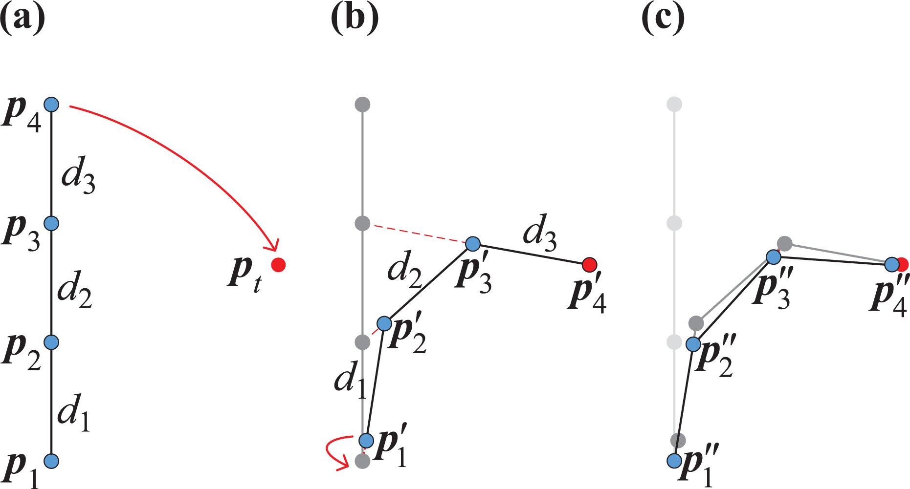
An example of a forward search and a backward search of FABRIK for a manipulator with four joints. (a) The positions of the manipulator and the target at the beginning of the movement. (b) Move the end effector
In the forward search, the end effector position of the manipulator
Relating FABRIK algorithm to velocity obstacles
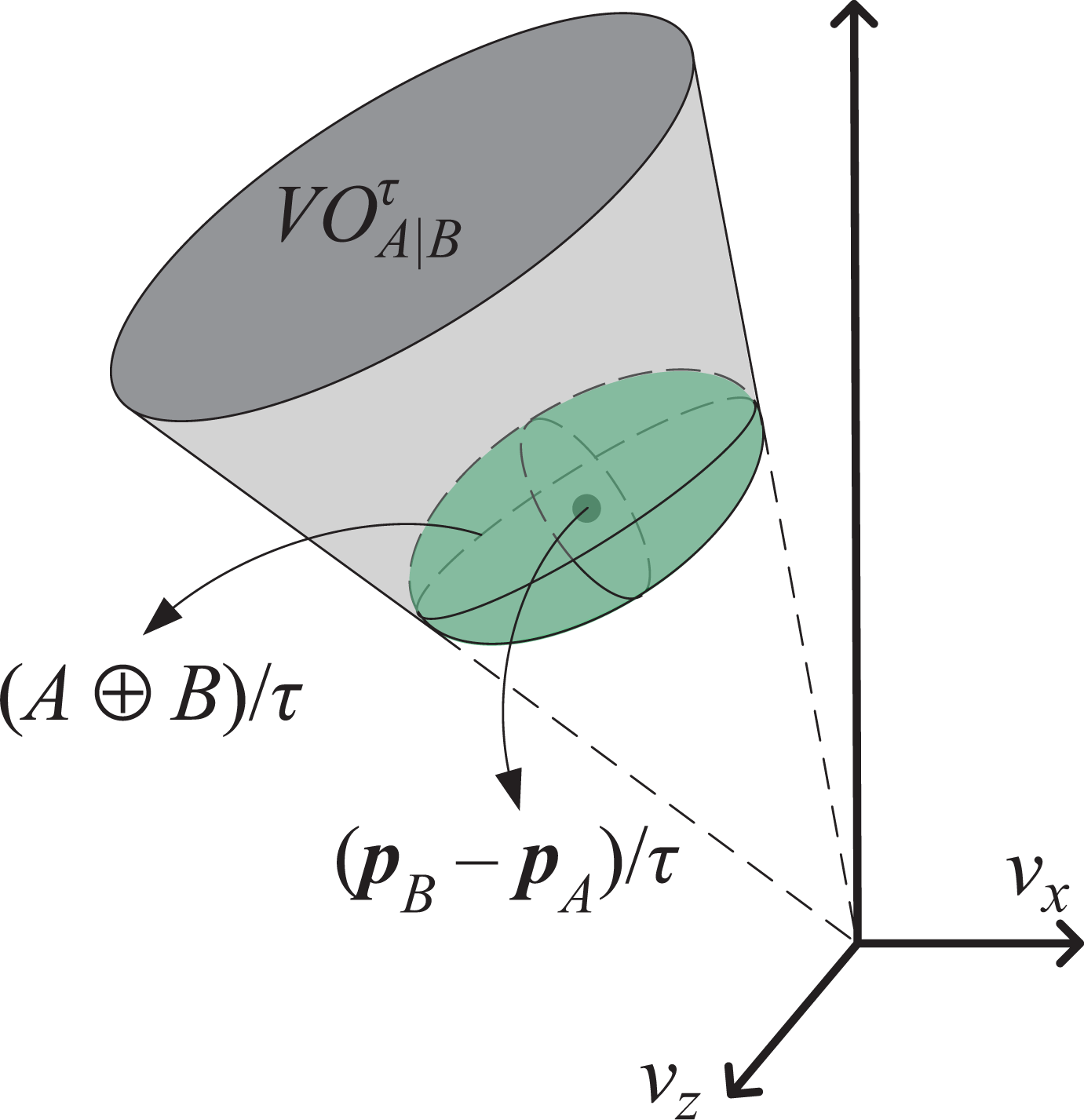
Given the method above, we would like to extend the notion of velocity obstacles to OA based on FABRIK. As shown in Figure 2, the ellipsoid A is represented by a center point


In the XYZ-dimensional, an ellipsoid and a sphere move toward one another with velocity
Let

where
The gray shaded area is the velocity obstacle for ellipsoid A induced by sphere B in time window
As shown in Figure 4, if the sphere B selects a velocity

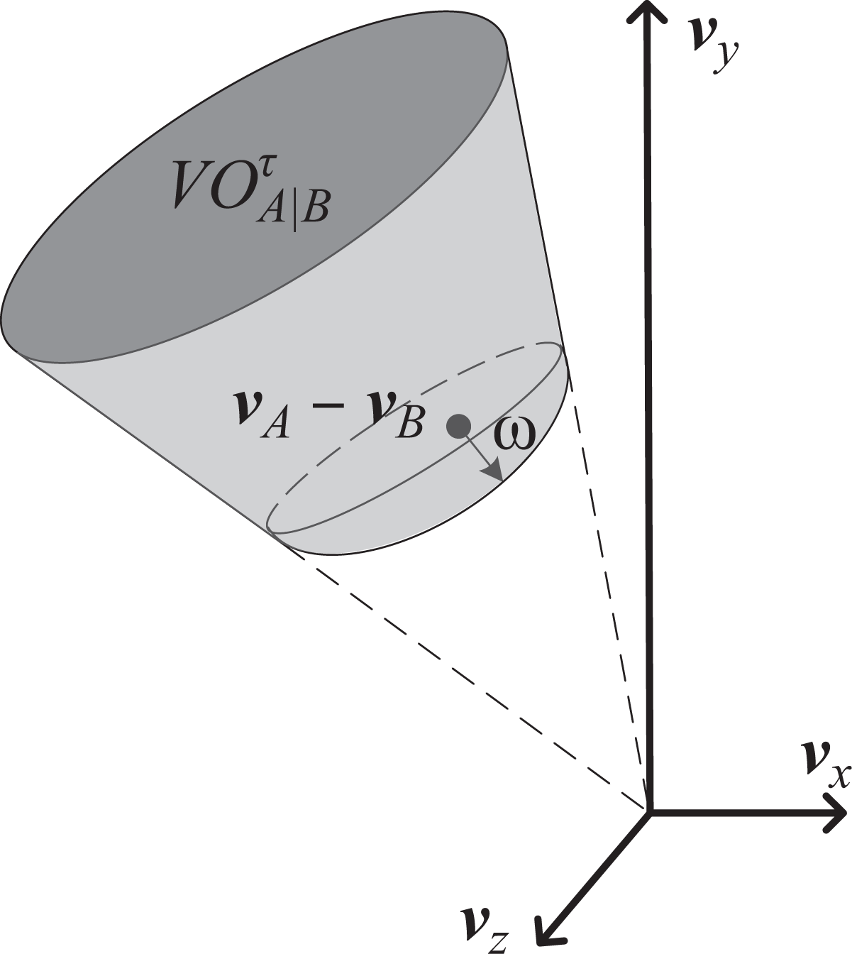
The vector
Given the defined generalized method for collision avoidance using velocity obstacles, we present the extension of this method for collision-free inverse kinematics for hyper-redundant manipulators. In FABRIK algorithm, we define a task error

To compute the joint position

where
An example for solving equation (6) is shown in Figure 5. We consider a hyper-redundant manipulator and a moving obstacle sharing a common working environment, where the obstacle moves with a known linear trajectory. The start positions of link I and moving obstacle are shown in Figure 5(a). Let
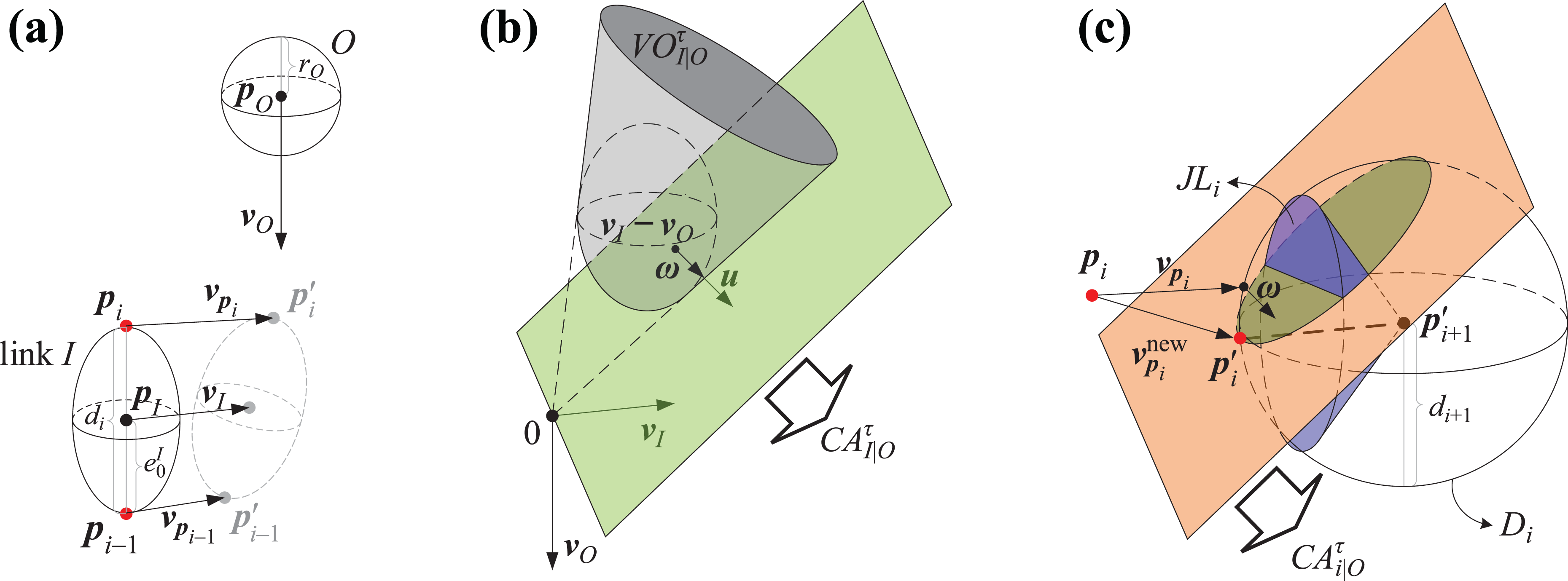
(a) In the XYZ-dimensional, the link I of a hyper-redundant manipulator and a dynamic obstacle are bounded by an ellipsoid and a sphere, respectively. (b) The gray-shaded area is the velocity obstacle
where
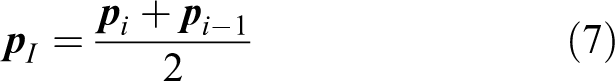
Figure 5(a) also shows the first step of the forward search in the FABRIK algorithm. Joint i updates its position to
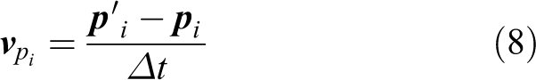
where

Then, the velocity obstacles

Since for link velocity, it holds that

and

where the two joints will share the responsibility for collision avoidance between the link I and the moving obstacle O equally. As shown in Figure 5(c),

Finally, joint i updates its position

and all other joints use the same approach to avoid collisions with the obstacles. For the backward search, apply the same method to the joints, and it would compute the set of feasible changes in velocity and update joint positions to avoid collisions with moving obstacles.
The detailed procedures of our approach for finding the inverse kinematic solutions based on FABRIK and velocity obstacles can be given in Algorithm 1. Moreover, Algorithm 1 terminates after
Collision-free inverse kinematic solution generator (our novel algorithm that accounts for task space, joint limit, and collision avoidance constraints)


If

that not only including distance constraint and/or joint limit constraint of joint i but also of the collision-free constraint in this search (forward or backward). Joint i updates its position using equation (14). The next link (i.e. link
The new velocity
The proposed algorithm has the consequence that if the moving obstacle potentially results in a collision with the hyper-redundant manipulator, then the changes in joint values will be computed to avoid this collision. This algorithm can be applied to general planar and spatial hyper-redundant manipulators with a single end effector for real-time control. It is able to compute collision-free inverse kinematic solutions that satisfy the complex dynamic constraints in the workspace and kinematic constraints (i.e. task space and joint limit constraints).
Implementation on special cases
We have introduced the above algorithm for collision avoidance for a hyper-redundant manipulator in an uncertain dynamic environment. We did so through a new algorithm of relating FABRIK algorithm to velocity obstacles. As shown in Algorithm 1, we can find a collision-free inverse kinematic solution for a hyper-redundant manipulator if given the position and velocity of the obstacle. We will now show how the previous algorithm of collision avoidance can be implemented in different working environments.
Avoiding collisions with multiple dynamic obstacles
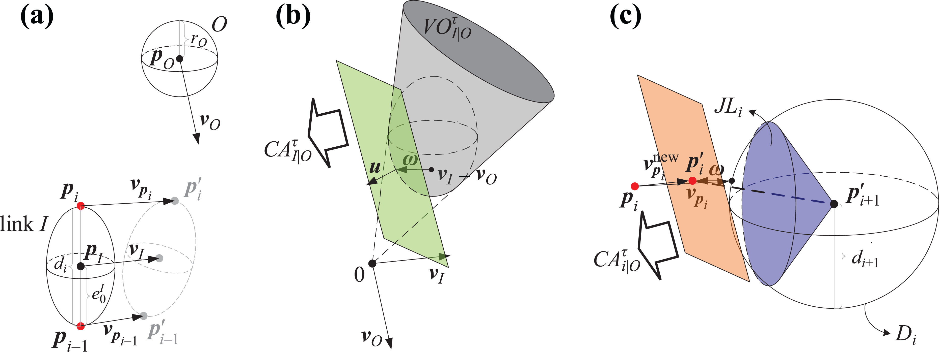
Algorithm 1 is presented for collision avoidance with one moving obstacle that can easily be extended to more than two obstacles. Let
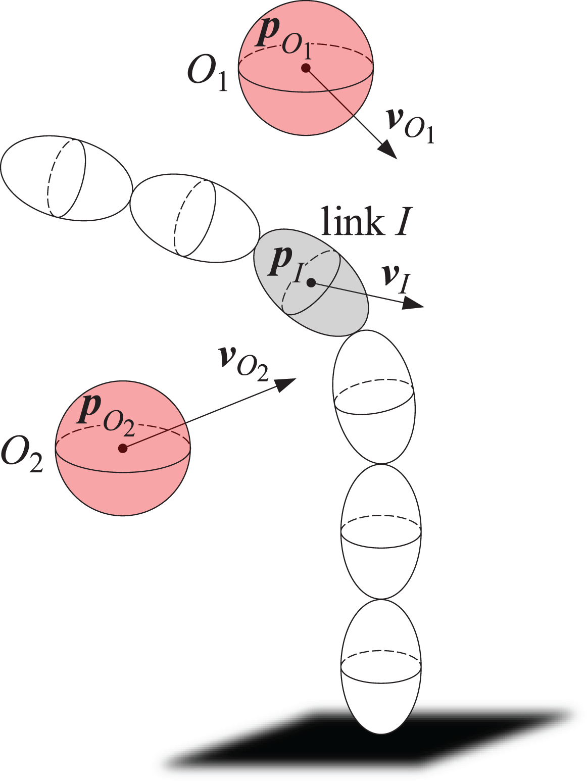
A case where a hyper-redundant manipulator and two moving obstacles O1 and O2 in the workspace.
Then, the velocity obstacles of the link I with respect to every obstacle can be defined using equation (3), as shown in Figure 8(a). The function

(a) The velocity obstacles and (b) the set
The set of safe changes in velocity for joint i can then be determined by
Since the only modification to Algorithm 1 is in the
Avoiding collisions with static obstacles
Algorithm 1 gives an inverse kinematic algorithm for the hyper-redundant manipulators and the moving obstacles to avoid collisions. However, the typical robot workspace also contains static obstacles, such as wall and pole. We will apply the same algorithm as above to this situation, it would compute the set
We assume that the geometric shape of the static obstacle is a regularly shaped body. More specifically, we would like to apply the basic space geometric shapes of cuboids and cylinders to model the static obstacles of walls and poles, respectively. This is shown in Figure 9. We can assume that the wall obstacle is modeled as a cuboid, and its geometric shape is determined by the position, orientation, and dimension of the wall obstacle. Let O be the cuboid, and let link I be an ellipsoid centered at

A case where a hyper-redundant manipulator and a static obstacle O in the workspace.

(a) The velocity obstacles
Implementation and performance
In this section, we highlight the performance of our algorithm in simulated environments that contain a hyper-redundant manipulator and many moving or static obstacles in the 2D and 3D workspaces. We present the kinematic parameters for hyper-redundant manipulators used in the simulations and the results from those simulations.
Implementation details
The simulations are developed in a C++ environment. The code runs on a single notebook running Ubuntu 16.04 64-bit with CPU i7-7700HQ at 2.81 GHz and 8GB RAM. To verify the adaptability of our approach, we run simulations that include the hyper-redundant manipulators with a different number of joints. The main structure of OA inverse kinematic scheme for hyper-redundant manipulators is shown in Figure 11. The simulations are initialized by decomposing the manipulator model into a series of ellipsoids (ellipses for planar manipulators). For simplicity, when the distance between the link and the obstacle is sufficiently large, we do not take this link into account while computing the collision-free constraint. The task space constraints are used to compute positioning error, and the velocity obstacles are used to define the safe velocity sets for each joint of the manipulator. A collision-free joint position

The obstacle avoidance inverse kinematic scheme for hyper-redundant manipulators.
Unless otherwise noted, we set a value of
Simulation results
Simulation A: Planar manipulator with a static obstacle
To illustrate our algorithm, we have provided a variety of simulations. In simulation A, the algorithm applied to a 7-DOF planar manipulator is compared with the shape trajectory control approach based on backbone curve
12
and the natural-cyclic coordinate descent (CCD) algorithm.
40
The simulation setup is shown in Figure 12. A 7-DOF planar manipulator (each joint has one DOF) and a circle-shaped obstacle are involved in this simulation. The black lines are the desired path of the end effector (i.e. joint position

Setup for simulation A.
The link length of the manipulator is
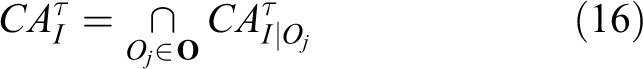
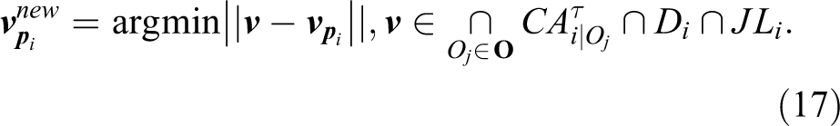
The selected screenshots of simulation A are shown in Figures 13 to 15. As can be seen, when the manipulators use the shape trajectory control approach (i.e. Figure 13) and the natural-CCD algorithm (i.e. Figure 14), it would lead to a collision with the obstacle during the operation. The configurations in Figure 15, with manipulator solving the inverse kinematics using our algorithm (i.e. OA-FABRIK), show no collisions over its entire operation. The joint trajectory computed by our algorithm in the manipulation phase in Figure 16 shows no sudden activation and no oscillation over its entire length.

(a–d) Shape trajectory control approach.
(a–d) Natural-CCD algorithm.
(a–d) Our collision-free inverse kinematic algorithm.

Angle variation for each joint for simulation A.
Simulation B: Spatial manipulator with dynamics obstacles
One set of simulations consists of a spatial hyper-redundant manipulator and groups of moving obstacles, where the manipulator and the obstacles were simulated separately. The setup of simulation B is shown in Figure 17. The workspace includes a 30-DOF manipulator with 10 joints (each joint has three DOF) and two moving obstacles, in which the velocity and position can be obtained. In this simulation, the manipulator tries to keep its end effector (i.e.

Setup for simulation B.
The parameters for the manipulator and the obstacles in this simulation are chosen as follows: the link length of the manipulator is
Based on the simulation setup, we performed three simulations, where one, two, and four moving obstacles cross the workspace with different velocity and direction, respectively. The manipulator can update its control input by the positions and velocities of those moving obstacles to avoid collisions. Selected screenshots of those simulations are shown in Figures 18 to 20.

(a–d) A simulation that contains a dynamic obstacle, which is a red sphere with velocity
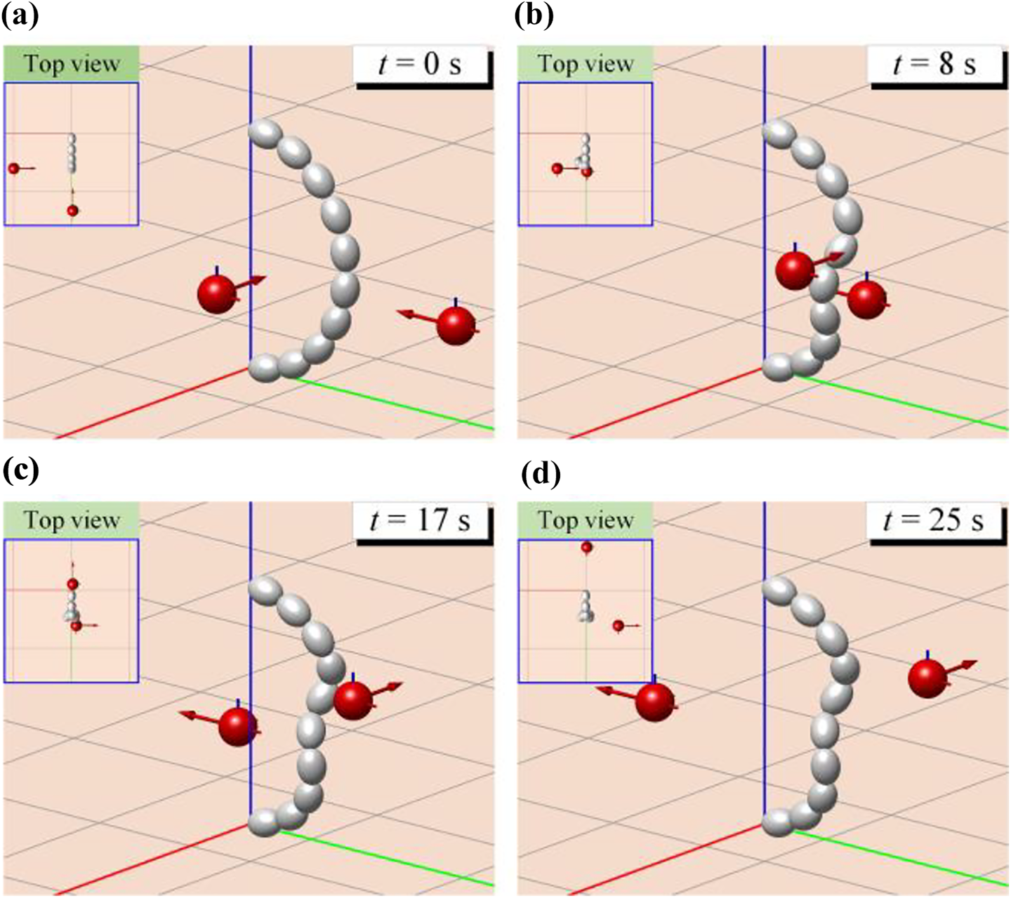
(a–d) A simulation that contains two dynamic obstacles with varying velocities. In the first screenshot, the velocity of left red sphere is
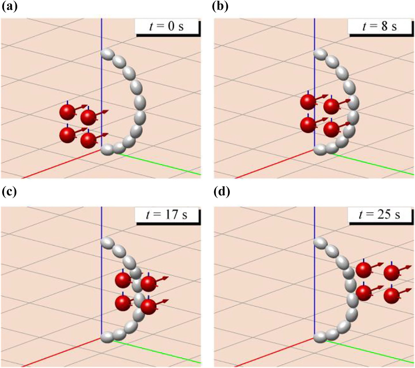
(a–d) A simulation that contains four dynamic obstacles. In the first screenshot, the velocities of two red spheres on the left are
Simulation C: Spatial manipulator with static obstacles
In simulation C, we test the performance of our algorithm on spatial hyper-redundant manipulator with the static obstacles. In this simulation setup, the typical static obstacles are used in the workspace. As shown in Figure 21(a) and (b), two challenging scenarios are presented, respectively, that is, scenario 1: a manipulator with 10 joints (each joint has three DOF) and a wall and a hole; and scenario 2: a manipulator with 19 joints (each joint has three DOF) and a cylindrical obstacle. In the simulations, a path planner of the end effector is needed, which has been given by the user. The joint motion command for the manipulator is generated based on our collision-free inverse kinematic algorithm.

(a, b) Setup for simulation C.
These two manipulators have the same kinematic parameters, which have been presented in simulation B. In addition, the desired velocity norm of the end effector during the simulations is

(a–d) A simulation in the scenario with a wall and a hole.

(a–d) A simulation in the scenario with a cylinder obstacle.
Performance analysis
Computational time
To quantify the computational time of our algorithm, we calculate the computation time of the inverse kinematic problem resolution, that is, the computation time it takes for one hyper-redundant manipulator to determine its joint positions of safe changes with respect to the moving or static obstacles in a single control cycle. As shown in Figure 24, the computation time grows with an increase in the number of moving obstacles and joints, as expected. In the simulation, we found that the safe velocity sets are computed without significantly increasing the computational time when the manipulator needs to avoid obstacles. As can be seen in Figure 24(b), the computational time also shows that for a single obstacle, the static obstacle could require a further increase in the computational time (at least in the workspace we implemented).

(a, b) The computational time of the inverse kinematic problem resolution is made for several number of simulations shown above.
Comparison
To further highlight the performance and efficiency of the proposed algorithm, the comparisons with some existing inverse kinematic approaches are listed in Table 1. It can be observed that the algorithms in the literature 17,39 do not consider the obstacles in the workspaces. In the literature, 7,15,18,33,37 although the proposed approaches can avoid collisions, they cannot be applied to the dynamic working environments. Moreover, the algorithms in Rolf et al. 17 and Safeea et al. 37 only apply to 2D workspaces. Note that the proposed algorithm can compute the collision-free inverse kinematic solutions in dynamic workspaces and can handle hyper-redundant manipulators. Furthermore, this algorithm is faster than other inverse kinematic algorithms, does not need any training, and can be applied in real-time control.
Comparisons among different inverse kinematic algorithms.

DOF: degrees of freedom.
a The algorithm is applied on a planar hyper-redundant manipulator.
b The algorithm is suitable for real-time control.
Conclusions
In this article, we present a novel method toward solving the inverse kinematic problem of hyper-redundant manipulators in complex working environments. To do so, we extend the notion of velocity obstacles to OA based on FABRIK. We then show how to implement the OA inverse kinematic algorithm in special cases. In our simulations, we see that the hyper-redundant manipulators can perform better OA using our algorithm.
The proposed approach has shown the expected performance of the collision-free kinematics for hyper-redundant manipulators in dynamic scenes. Due to the structural characteristic of soft manipulators, 41,42 a future line of research will be focused on the integration of our algorithm with the soft robotic arm by converting the discrete inverse kinematic solutions to continuous curves. Moreover, we would like to evaluate the performance in dynamic scenes with human or other complex obstacles.
Footnotes
Declaration of conflicting interests
The author(s) declared no potential conflicts of interest with respect to the research, authorship, and/or publication of this article.
Funding
The author(s) disclosed receipt of the following financial support for the research, authorship, and/or publication of this article: This work was supported by the National Natural Science Foundation of China [Project Number: 91848101 and 51805107] and the Foundation for Innovative Research Groups of the National Natural Science Foundation of China [Grant Number: 51521003].
Supplemental material
Supplemental material for this article is available online.
References
Supplementary Material
Please find the following supplemental material available below.
For Open Access articles published under a Creative Commons License, all supplemental material carries the same license as the article it is associated with.
For non-Open Access articles published, all supplemental material carries a non-exclusive license, and permission requests for re-use of supplemental material or any part of supplemental material shall be sent directly to the copyright owner as specified in the copyright notice associated with the article.