Sage Journals: Discover world-class research

Abstract

Industrial robots are getting widely applied due to their low use-cost and high flexibility. However, the low absolute positioning accuracy limits their expansion in the area of high-precision manufacturing. Aiming to improve the positioning accuracy, a compensation method for the positioning error is put forward in terms of the optimization of the experimental measurement space and accurate modelling of the positioning error. Firstly, the influence of robot kinematic performance on the measurement accuracy is analysed, and a quantitative index describing the performance is adopted. On this basis and combined with the joints motion characteristics, the optimized measurement space in joint space as well as Cartesian space is obtained respectively, which can provide accurate measurement data to the error model. Then the overall model of the positioning error is constructed based on modified Denavit–Hartenberg method, in which the geometric errors and compliance errors are considered comprehensively, and an error decoupling method between them is carried out based on the error-feature analyses. Experiments on the KUKA KR210 robot are carried out finally. The mean absolute positioning accuracy of the robot increases from 1.179 mm to 0.093 mm, which verifies the effectiveness of the compensation methodology in this article.

Keywords

Industrial robot positioning error kinematic performance optimized measurement space error decoupling

Introduction

Industrial robots are getting widely used in more and more industrial applications gradually because of their prominent advantages such as the low use-cost and high flexibility. Not limited to the simple jobs such as pick-and-place, they also find their niche in manufacturing operations such as deburring and drilling, which require special attention to the manufacturing accuracy.¹

The trend is that modern industrial robots will someday replace the less flexible and costlier computer numerical control (CNCs) in many areas. However, there are some obstacles such as the low absolute positioning accuracy. The absolute positioning accuracy of robots is generally larger than 0.3 mm, which can hardly satisfy the requirement of high-precision machining and greatly limits their application scope.² Up to the present time, the applications of the robots in high-precision machining are relatively few.

Aiming at improving the absolute positioning accuracy, extensive studies have been implemented as listed in Table 1. According to the calibration mode, there exist mainly two kinds of methods, namely the model-based parameter calibration method and the non-parameter one. The latter one requires higher experimental design and measurement process, which is of high cost and makes it of less application. Therefore, most of the current studies are based on the model-based parameter calibration.^3

–6 Generally speaking, four steps are contained in this calibration procedure: modelling, measurement, identification and implementation. The aim of the first step is to develop a model to establish the relationship between the actual and designed positions of the robot end-effector (EE), which is the basis of the calibration and has a high requirement for its completeness and accuracy. At the measurement step, the actual position data of the robot EE are obtained through the measuring instruments based on open-loop and closed-loop methods in general. The identification step is aimed at solving the parameter errors according to the model and the experimental data. The compensation of the positioning error is dealt with in the last step of implementation. There exist two common methods for the compensation, which are the modification of input parameters as well as the robot control software. The first one is more widely used for its convenience.

Table 1.

Major research efforts in improving the absolute positioning accuracy.

Authors	Research object	Method	Absolute positioning accuracy (mm)
Authors	Research object	Method	Before calibration	After calibration
Gong et al.³	6-DoF industrial robot	Kinematic model + non-geometric error identification	1.2	0.11
Shen et al.⁵	6-DoF industrial robot	Position and deformation errors compensation	0.677	0.134
Chen et al.⁶	Kuka robot	Kinematic model + co-kriging method	0.7168	0.1150
Klimchik et al.⁸	Kuka KR-270 robot	D-optimality principle + optimal pose selection	2.29	0.14
Borm et al.⁹	PUMA-type robots	Kinematic model + observability measure criterion	5.157	0.7009

As far as the author’s knowledge, the existing literatures mainly focus on the aspects of modelling and parameter identification, while studies on measurement methods are limited, especially on the choice of measurement space. Studies have found that the difference in working spaces has an important impact on the robot performance. Many kinds of indexes have been proposed for the performance evaluation, among which singularity is the most common used indicator. When the robot EE is close to the singular point, its speed and motion will be greatly out of control and the EE position is difficult to guarantee, which will result in the inaccuracy of measurement data, further leading to the error of parameters identification and reducing the accuracy of robot calibration.^7,8 Borm and Meng showed that compared with merely increasing the experiments number, an appropriate selection of the measurement configuration is more crucial and economical in robot calibration.⁹ A strategy for the selection of optimal measurement configuration is proposed by Klimchik et al.¹⁰ The results showed that the efficiency of robot calibration can be increased adopting this strategy. The condition number of Jacobian matrix is used to evaluate the robot performance in the study by Zargarbashi et al.¹¹ They found that it is essential to keep the robot EE far away from the positions of singularity for the reason that the joint rates are easy to get out of control at singularities, which can affect the accuracy of motion.

From the literatures above, it can be concluded that the difference in measurement space can affect the calibration accuracy to a certain extent. In addition, the planning of the robot motion trajectory is mostly based on the optimized workspace, which is mostly defined as the space far away from the singular.¹² Therefore, it is reasonable and necessary to calibrate the robot positioning accuracy based on the optimized workspace.

Based on the above analyses, a compensation method for absolute positioning error of industrial robots is put forward in this article, which not only considers the accurate modelling of the positioning error but also takes fully consideration of the optimized measurement space. The main parts are arranged as follows. Section of ‘The optimized space based on the kinematic performance index’ describes the discrimination method of the optimized space based on kinematic performance index, and the optimized measurement space in joint space as well as Cartesian space is given respectively. Section of ‘The model of the robot positioning error’ constructs an overall model of the robot positioning error, where the geometric errors and compliance errors are modelled and decoupled based on their features. The error compensation method is given in the section of ‘The error compensation method’. Experiments based on a robotic platform were carried out in the section of ‘Experiments and discussion’, which will verify the effectiveness of the methods in this article. Finally, the ‘Conclusions’ section summarizes the main work and contributions.

The optimized space based on the kinematic performance index

As seen from previous investigations, the measurement space affects the positioning accuracy greatly. Therefore, in this part, a kinematic performance index based on the Jacobian condition number is first put forward, which is the discrimination method for the optimized space. Further, through the analyses of the characteristics of robot joints motion, the optimized measurement space in joint space as well as Cartesian space is obtained, which will provide support for the selection of measurement space.

The kinematic performance index

The kinematic performance index is an index that can measure the motion performance regarding the motion transmission of robots. Jacobian matrix J(q) describes the mapping relationship between the infinitesimal rotation amount of the joints and the resulting displacement of the EE, which makes it an important factor in the construction of the kinematic performance index. In fact, when $|J (q)| = 0$ , this robot is in a singular position. As for the singular position, there exist two situations for the joint rates under a given EE speed: (1) non-existent and (2) quite large. Both of them will lead to a bad motion performance, which will affect the accurate position control of the robot.

The Jacobian matrix is a posture-dependent function, which means that its value depends on the robot’s spatial posture. Therefore, it is widely used in the literature to construct different indicators to describe the motion performance of robots in different spaces. Among them, the reciprocal of the Jacobian condition number (which is called the kinetostatic conditioning index (KCI)) is the most commonly used as shown in equation (1), which can characterize the distance to the singular point.¹³ The larger the KCI is, the better dexterity and control accuracy the robot achieves

\begin{array}{l} KCI = \frac{1}{k (J_{N})} \times 100 %, J_{N} \in R^{m \times n}, m \leq n \\ k (J_{N}) = \frac{1}{m} \sqrt{t r (J_{N} J_{_{N}}^{T}) t r ({(J_{N} J_{_{N}}^{T})}^{- 1})} \end{array}

where $k (J_{N})$ represents the condition number of the homogeneous Jacobian, the subscript N and tr(·) denote the normalizing operation as well as the matrix trace. And J_N is expressed as

J_{N} = [\begin{matrix} \frac{1}{L} I_{3 \times 3} & O_{3 \times 3} \\ O_{3 \times 3} & I_{3 \times 3} \end{matrix}] J

where $O_{3 \times 3}, I_{3 \times 3}, a n d J$ represent null matrix, unit matrix, and Jacobian matrix, respectively. L is the characteristic length used to normalize the Jacobian matrix, which can ensure the same physical unit of all the items of Jacobian matrix. L can be obtained by solving the maximum of KCI.¹³

The optimized measurement space based on KCI

Known from the definition of KCI, the optimized measurement space is the space where KCI is bigger than a certain lower limit, which should be determined by the practical application scenarios. Therefore, in this part, the distribution characteristics of KCI in different spaces are analysed based on the joints motion, and further the optimized measurement space in joint space as well as Cartesian space is obtained.

Industrial robots are generally six-axis series mechanism. For the convenience of description, we name the joints from the base as J1–j6 and the axes as Z1–Z6. According to the corresponding research conclusions, j1 has no effect on the kinematic performance of robots, which means only j2–j6 need to be optimized. Among them, j2 and j3 mainly affect the position of the robot EE, while j4–j6 mainly affect the orientation of the robot EE.¹⁴ Therefore, they will be analysed separately.

Specifically analysed from the singularity, on the condition that Z4 is not parallel to Z6, a good kinematic performance can be obtained. So according to the structural features of robot joints, only if j5 is not equal to 0, the singularities in j4–j6 can be prevented. Combined with the parameter characteristics of the robot joints in this article (see Table 2), the range of j5 is set to be [−125, −30] and [30, 125] (degree) which will guarantee j4–j6 far from singularity. j4 and j6 will not be affected and are still in their motion boundaries.

Table 2.

The joints parameters of KUKA KR210.

Joint i	θ (°)	d_i (mm)	α_i (°)	a_i (mm)	θ range (°)
1	$θ_{1}$	750	0	0	−185 to +185
2	$θ_{2}$	0	−90	350	−146 to +110
3	$θ_{3}$	0	0	1250	−209 to +85
4	$θ_{4}$	1100	−90	−55	−350 to +350
5	$θ_{5}$	0	90	0	−125 to +125
6	$θ_{6}$	230	−90	0	−530 to +170

As for the joints of j2 and j3, the motion ranges can be determined according to the KCI map. It can be seen from the foregoing analyses that the singularity of j2–j3 is not affected by j4–j6 under the premise that j4–j6 are not singular. Therefore, for the sake of convenience, the specific values of j1, j4, j5 and j6 are set to be 0°, 0°, 45° and 0°, respectively. Under this setting and by the use of equation (1), the KCI map can be depicted, based on which the influence law of singularity for j2 and j3 is presented. The KCI map for j2 and j3 in the joint space can be seen in Figure 1(a). According to the nature of the KCI, that is, the larger the KCI is, the farther the EE is from the singularities, and the better the kinematic performance is. Here, the threshold value of KCI is selected to be 0.35. When KCI is larger than 0.35, the robot is in the optimized space. The optimized measurement space in joint space as well as Cartesian space is shown in the area of Z_o in Figure 1((a) and (b)). Accordingly, we can obtain the ranges of j2 and j3 satisfying the performance requirements, which are [−114, 40] and [−30, 60] (degree).

Figure 1.

The kinematic performance maps: (a) In the joint space and (b) in the Cartesian space.

The model of the robot positioning error

It has been proved that the maximum error of robots is the geometric error, which contributes no less than 80% of the total error.³ While due to the compliance of the robot links and joints, the compliance error of the EE cannot be overlooked either.^15,16 There is the coupling effect between them and the compliance errors vary with the posture of the EE all the time, which lead to a difficulty in distinguishing them two. Most studies merely take the geometric errors as the object and ignore the existence and variability of the compliance errors, which is hard to build a precise error model and makes the results inaccurate.

As for the problem above, in this part, the overall model of the positioning error is constructed adopting modified Denavit–Hartenberg (MD-H) method. Further, geometric errors and compliance errors are considered comprehensively, and the error decoupling method between them is carried out based on the feature analyses, which can improve the accuracy of the error model.

The overall model of positioning error

Most of the existing error models are based on kinematics. By measuring the error between the theoretical and actual positions of the robot EE, the parameter errors can be obtained by the inverse operation of the kinematics. Therefore, a robot kinematics model is needed in the first place. In this article, MD-H method is adopted and a rotational parameter about the y-axis is introduced on the basis of the original Denavit–Hartenberg (D-H) method, which can deal with the singularity phenomenon caused by the parallelism of the adjacent joints. The transform equation between the successive reference systems can be expressed as¹⁷

A_{i}^{i - 1} = Trans (Z, d_{i}) Rot (Z, θ_{i}) Trans (X, a_{i}) Rot (X, α_{i}) Rot (Y, β_{i})

where $A_{i}^{i - 1}$ is the transform formula from joint i to i − 1, $d_{i}, θ_{i,} a_{i,} α_{i,} β_{i}$ represent the distance from $x_{i - 1}$ to x_i along z_i , the angle from $x_{i - 1}$ to x_i about z_i , the distance from $z_{i - 1}$ to z_i along $x_{i - 1}$ , the angle from $z_{i - 1}$ to z_i about $x_{i - 1}$ and the twist angle about y_i , respectively.

Here set that $Δ d_{i}, Δ θ_{i}, Δ a_{i}, Δ α_{i}, Δ β_{i}$ represent the tiny errors of $d_{i}, θ_{i}, a_{i}, α_{i}, β_{i}$ , respectively, which include geometric and compliance errors in all. And then according to MD-H method, the actual transform formula from EE to the base coordinate system can be expressed as

{}^{'}T_{N} = \prod_{i = 1}^{N} {}^{'}A_{i}^{i - 1} = \prod_{i = 1}^{N} (A_{i}^{i - 1} + δ A_{i}^{i - 1})

where ${}^{'}A_{i}^{i - 1}$ is the transform formula from joint i to i − 1 regarding the tiny errors and $δ A_{i}^{i - 1}$ represents the tiny errors from joint i to i − 1.

When $δ A_{i}^{i - 1}$ is tiny, a simple linear formula can be obtained as¹⁸

δ A_{i}^{i - 1} = \frac{\partial A_{i}^{i - 1}}{\partial θ_{i}} Δ θ_{i} + \frac{\partial A_{i}^{i - 1}}{\partial d_{i}} Δ d_{i} + \frac{\partial A_{i}^{i - 1}}{\partial α_{i}} Δ α_{i} + \frac{\partial A_{i}^{i - 1}}{\partial β_{i}} Δ β_{i} + \frac{\partial A_{i}^{i - 1}}{\partial a_{i}} Δ a_{i}

Based on equations (4) and (5), the high-level minim can be omitted, and then the error between the actual and ideal positions can be obtained as follows

Δ P = P^{'} - P = \sum_{i = 1}^{N} \frac{\partial T_{N}}{\partial θ_{i}} Δ θ_{i} + \frac{\partial T_{N}}{\partial d_{i}} Δ d_{i} + \frac{\partial T_{N}}{\partial α_{i}} Δ α_{i} + \frac{\partial T_{N}}{\partial β_{i}} Δ β_{i} + \frac{\partial T_{N}}{\partial a_{i}} Δ a_{i}

where $\frac{\partial T_{N}}{\partial v_{i}} = A_{2}^{1} A_{3}^{2} ... \frac{\partial A_{_{i}}^{i - 1}}{\partial v_{i}} ... A_{_{N}}^{N - 1}$ , v represents the set of joints parameters, namely $d_{i}, θ_{i,} a_{i,} α_{i,} β_{i}$ .

Further arrange equation (6), it can be expressed in the matrix form as

[\begin{matrix} Δ D \\ ΔΘ \end{matrix}] = [\begin{matrix} M_{d} \\ 0 \end{matrix}] Δ d + [\begin{matrix} M_{θ} \\ R_{θ} \end{matrix}] Δ θ + [\begin{matrix} M_{a} \\ 0 \end{matrix}] Δ a + [\begin{matrix} M_{α} \\ R_{α} \end{matrix}] Δ α + [\begin{matrix} M_{β} \\ R_{β} \end{matrix}] Δ β

where $Δ D$ and $ΔΘ$ represent the deviations of position and orientation, respectively, $M_{θ}, M_{d}, M_{a}, M_{β}, M_{α}$ are 3 × N matrices of partial derivatives of the EE position regarding the kinematic parameter errors, $R_{θ}, R_{β}, R_{α}$ are 3 × N matrices of partial derivatives of the EE orientation regarding the kinematic parameter errors.

A more compact format of equation (7) can be expressed as

Δ P = J_{I} Δ V

where $Δ V$ represents the set of joint parameter errors, namely

Δ V = (Δ d, Δ θ, Δ a, Δ α, Δ β) = Δ V_{g} + Δ V_{c}

where $Δ V_{g} = (Δ d_{g}, Δ θ_{g}, Δ a_{g}, Δ α_{g}, Δ β_{g})$ represents the geometric errors, $Δ V_{c} = (Δ d_{c}, Δ θ_{c}, Δ a_{c}, Δ α_{c}, Δ β_{c})$ represents the compliance errors, and J_I is the identification Jacobian matrix and can be written as

J_{I} = (\begin{matrix} M_{θ} M_{d} M_{a} M_{α} M_{β} \\ R_{θ} 0  0 R_{α} R_{β} \end{matrix})

As for the measurement, the laser tracker is widely used. While the base coordinate constructed by the laser tracker cannot be the same with real coordinate and there is a transform error between them.¹⁸ To reduce the transform error, a transform matrix between the two coordinate systems is introduced here

{}^{'}E = [\begin{matrix} 1 & - r_{z} & r_{y} & d_{x} \\ r_{z} & 1 & - r_{x} & d_{y} \\ - r_{y} & r_{x} & 1 & d_{z} \\ 0 & 0 & 0 & 1 \end{matrix}]

where $d_{x}, d_{y}, d_{z}$ are the tiny distance errors along X-, Y-, Z-axes between the two coordinate systems and $r_{x}, r_{y}, r_{z}$ are the tiny rotational angle errors about X-, Y-, Z-axes.

Therefore, taking the transform error into consideration, the positioning error under a certain posture can be obtained by

\begin{array}{l} Δ P^{m} = P^{m} - P = {}^{'}E P^{'} - P = {}^{'}E (P + Δ P) - P = ({}^{'}E - E) P + Δ P + ({}^{'}E - E) Δ P \end{array}

where E is the unit matrix and $({}^{'}E - E) ΔP$ is omitted for its high-level minim. Then equation (10) can be simplified to

Δ P^{m} = ({}^{'}E - E) P + Δ P

Based on the equations above, and under the condition that the EE displacements $Δ P^{m}$ as well as the identification Jacobian matrix J_I is known, the overall joint parameter errors of the robot can be solved.

Compliance errors modelling

The compliance errors are mainly caused by the deformation of the joints, links as well as transmission system under the action of forces, mainly referring to the robot gravity in this part. For the convenience of analysis, based on the previous research conclusions, the following two assumptions are made before modelling^19,20:

The links are considered to be rigid, regardless of theirs compliance errors.

Since the torsion angles of the joints caused by external force are small, the relationship between them can approximate to be linear.

Based on the two assumptions, the following compliance errors formula can be obtained as

Δ θ_{c i} = C τ

where $Δ θ_{c i}$ represents the torsion angle caused by the robot gravity, C is the elasticity coefficient with a fixed value for a certain joint and τ means the torque on the joint.

It is known that the robot gravity mainly comes from the weight of the robot links, among which the second and third links are the heaviest. Therefore, the biggest torques are applied on j2 and j3, leading to the biggest compliance errors.¹⁵ For simplicity, omitting the gravity of other links, the compliance error model can be further simplified by only considering the compliance errors of j2 and j3.

Then the parameters in equation (12) are solved next.

The elasticity coefficient C is the reciprocal of the stiffness coefficient K of the joint. There are generally two methods in solving K. The first method is clamping all the joints except the one to be measured and the second one measures the displacements of the EE due to certain forces and evaluates K throughout its Cartesian workspace. The latter method is more convenient and can provide a good approximation when the experiments are enough, which is adopted in this article.

The solution formula for K is as follows¹⁴

F = J^{- T} K_{q} J^{- 1} Δ x_{t}

where F is the load on the EE, $Δ x_{t}$ is the displacements of the EE and K_q is the 6 × 6 diagonal stiffness matrix.

The numerical calculation method of equation (13) can refer to the literature.¹⁴

As shown in Figure 2, G and L represent the barycenter and length of the robot link, respectively, and $θ_{2}$ and $θ_{3}$ are the link angles relative to the vertical and horizontal lines. Then according to equation (12), the torsion angle of j2 caused by the gravity can be calculated by

Δ θ_{c 2} = C_{2} (G_{2} L_{2} / 2 + G_{3} L_{2}) sin θ_{2} + C_{2} G_{3} L_{3} cos θ_{3} / 2

By the same token, the torsion angle of j3 is obtained by

Δ θ_{c 3} = C_{3} G_{3} L_{3} cos θ_{3} / 2

Figure 2.

The schematic diagram of compliance errors caused by gravity.

Geometric errors decoupled from compliance errors

It can be known from equation (8) that the overall joint parameter errors are the superposition of geometric errors and compliance errors. Therefore, the geometric errors can be decoupled by subtraction of the overall joint parameter errors and compliance errors. Then the solution formula for the geometric errors is as follows

\begin{matrix} Δ V_{g} = Δ V - Δ V_{c} = (Δ d, Δ θ, Δ a, Δ α, Δ β) - (0, Δ θ_{c}, 0, 0, 0) \\ = (Δ d, Δ θ - Δ θ_{c}, Δ a, Δ α, Δ β) \end{matrix}

where $Δ θ_{c} = {(0, Δ θ_{c 2}, Δ θ_{c 3}, 0, 0, 0)}^{T}$ .

The error compensation method

Based on the work above, the error compensation process is given as shown in Figure 3.

Determine the optimized measurement space based on the kinematic performance index, which will be the experimental space for the robot calibration;

Carry out the calibration experiments for the compliance errors, and the elasticity coefficients of the robot joints j2 and j3 are obtained in this step;

Collect the position information in the optimized measurement space and solve the overall joint parameter errors;

Solve the geometric errors of the robot by subtraction of the overall parameter errors and real-time compliance errors;

Correct the nominal robot joints parameters according to the calculated errors and obtain the new set of parameters; and

Carry out the verified experiments based on the new joints parameters. Stop when the positioning accuracy meets the requirements, otherwise return to step 3.

Figure 3.

The flowchart of the error compensation method.

Experiments and discussion

Setup of the experiments

The experimental devices for the robot positioning accuracy calibration are shown in Figure 4. The industrial robot of KUKA KR210 is adopted in the experiments. This robot is a medium-sized six-axis robot produced by KUKA of Germany, which has obvious features and wide application range. The parameters related to this type of robot are presented in Table 2. The EE coordinates are measured by the third generation laser tracker of American API Company, whose resolution is up to 1 µm and can meet the experimental precision requirements.

Figure 4.

The experimental devices for the robot positioning accuracy calibration.

Before the experiments, the robot base coordinate system is first constructed using the laser tracker, and then the actual coordinates of the robot EE at different positions are measured. The measurement process is:

Set up the measurement experiment platform, as shown in Figure 4.

Install the laser tracker, place the target ball at the EE and preheat the tracker power for 15–45 min to ensure measurement accuracy.

Install the SpatialAnalyzer. V2015 software, import the robot ontology model and set the relevant measurement parameters as needed.

Move the robot EE and acquire the position information.

Identification of the parameter errors

1. The compliance errors identification

Based on the error compensation process, the elasticity coefficients of the robot joints j2 and j3 are first to be determined. In the optimized measurement space as shown in Figure 1(b), the displacements of the EE under certain applied loads are measured using API. Then according to equations (13 ) to (15), the elasticity coefficients of joints j2 and j3 are obtained as follows

\begin{array}{l} C_{2} = 7.0223 \times 10^{- 7} {(N \cdot m)}^{- 1} \\ C_{3} = 5.7906 \times 10^{- 6} {(N \cdot m)}^{- 1} \end{array}

Then as shown in Figure 5, the compliance errors $Δ θ_{c 2}$ and $Δ θ_{c 3}$ under different rotational angles can be depicted.

Figure 5.

$Δ θ_{c 2}$ and $Δ θ_{c 3}$ under different rotation angles of joints j2 and j3: (a) $Δ θ_{c 2}$ and (b) $Δ θ_{c 3}$ .

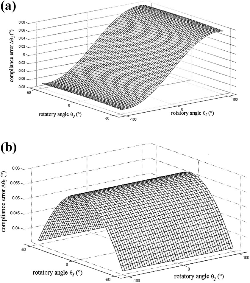
As shown in Figure 5, the compliance errors are posture-dependent. The error of the torsion angles can reach as big as 0.07°, which is almost equal to the geometric error of α for j4 (see Table 3). Therefore, the compliance errors are significant and should be considered to improve the robot positioning accuracy.

Table 3.

The geometric errors of KUKA KR210.

Number	θ (°)	d (mm)	a (mm)	α (°)	β (°)
1	−0.002 15	0.260 03	−0.172 06	0.11715	0
2	−0.072 46	−0.411 25	0	0.410 16	0.004 92
3	0.481 73	0.102 36	−0.209 31	−0.301 21	0
4	−0.247 04	0.005 46	0.401 24	0.079 36	0
5	0.041 35	−0.562 31	0.001 05	−0.092 28	0
6	−0.171 34	−0.300 25	0	0.017 45	0
Others	r_x = 0.002 05°, r_y = 0.003 75°, r_z = −0.002 34°, d_x = 0.542 43 mm, d_y = −0.097 77 mm d_z =0.435 38 mm

2. The geometric errors identification

Seventy groups of the position coordinates are recorded in this article, of which 40 are used for errors identification and the others for verification. And to improve the accuracy, the positions are scattered as much as possible in the optimized measurement space. According to the error models, the geometric errors are identified and shown in Table 3.

Verification of the errors compensation method

Based on the section of ‘The model of the robot positioning error’, the robot joints parameters, including geometric errors and compliance errors, are known. Then according to the error compensation process, the compensation experiments were carried out. To validate the effectiveness of the method, four groups of experiments were implemented.

1. Compensation experiments without considering compliance errors

In this group of experiments, the parameters obtained from the overall error model are treated as the geometric errors only, which means the compliance errors are not considered. Under this assumption, the results before and after error compensation are shown in Figure 6.

Figure 6.

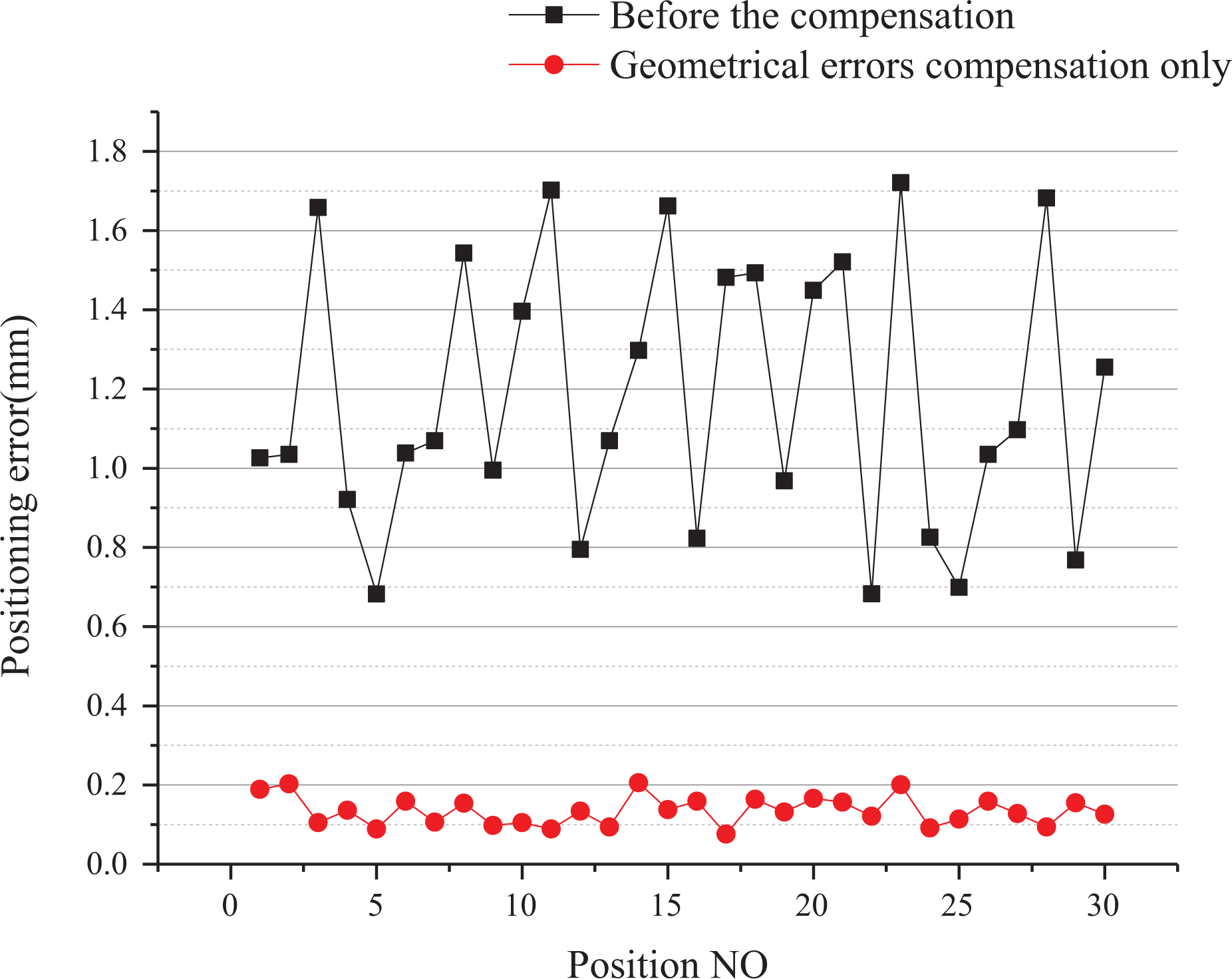
The error results before and after the geometric errors compensation only.

As shown in Figure 6, the mean positioning accuracy of the 30 positions for verification is reduced from 1.179 mm to 0.135 mm, and the maximum positioning accuracy error is reduced from 1.721 mm to 0.206 mm after the overall errors are compensated. Therefore, the error compensation for the robot is of great significance, which can greatly improve its positioning accuracy.

2. Compensation experiments considering compliance errors

In this group of experiments, the geometric errors and compliance errors are both considered. And the results before and after error compensation are shown in Figure 7.

Figure 7.

The error results before and after the compliance errors compensation.

As shown in Figure 7, compared with the compensation based on the geometric errors only, the mean positioning accuracy of the 30 positions for verification is reduced from 0.135 mm to 0.093 mm and the maximum positioning accuracy error is reduced from 0.206 mm to 0.126 mm by considering compliance errors. Therefore, the error compensation method considering compliance errors can improve the robot positioning accuracy better.

3. Verification experiments of the optimized measurement space

Replace 20 groups of measured positions in the optimized measurement space by those in the unoptimized space and identify the parameter errors based on the new data. Then the new identified parameters are adopted for the error compensation. The compensation results are shown in Figure 8.

Figure 8.

The error results within and out of the optimized space.

As we can see from Figure 8, the mean positioning accuracy is reduced from 0.117 mm to 0.093 mm, and the maximum positioning accuracy error is reduced from 0.164 mm to 0.126 mm by choosing the positions in the optimized space. Therefore, the identified parameters in the optimized space are of more accuracy and can better improve the robot positioning accuracy, which verifies the method in this article.

4. Comparisons between the proposed method and other methods

The maximum and mean positioning errors of the proposed method and other methods in Table 1 are listed in Table 4. The methods of the literature^3,6 are based on the kinematic model, and the application objects are both six-axis serial robots, which are the same as those in this article. Therefore, the methods of the literature^3,6 are specifically selected for comparison. The same 40 groups of positions in the section of ‘Verification experiments of the optimized measurement space’, which contain 20 groups in the non-optimized space and 20 in the optimized space, are chosen as the measurement points for the methods of the references.

Table 4.

Comparisons between the proposed method and other methods.

Authors	Method	Absolute positioning accuracy (mm)
Authors	Method	Maximum error	Mean error
Gong et al.³	Kinematic model + non-geometric error identification	0.131	0.089
Chen et al.⁶	Kinematic model + co-kriging method	0.241	0.128
This article	Kinematic model +optimal measurement space selection	0.126	0.093

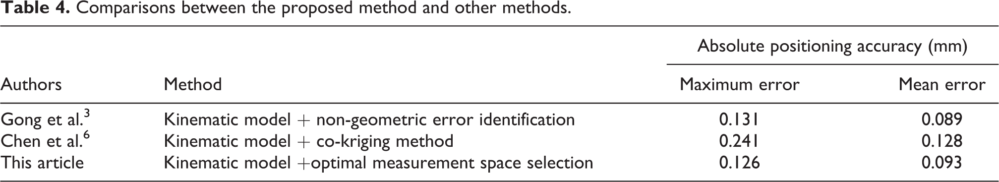
The co-kriging method in the study by Chen et al.⁶ is a kind of regression algorithm based on interpolation, whose prediction accuracy is greatly related to the sample size and the correlation between the samples. The larger the sample size is and the greater the correlation is, the higher accuracy the method can achieve. In addition, the calculation process involves the determination of the sample weight function, which also greatly affects the accuracy of the results. The above-mentioned factors lead to a complicated calculation process and large volatility of the results. Therefore, due to the strong non-linearity of spatial error distribution and the small sample size in this article, the compensation accuracy of the co-kriging method is relatively low. The method in the study by Gong et al.³ established a comprehensive error model including geometric and non-geometric errors. While the measurement errors are not taken into consideration, which will decrease the compensation accuracy and has been proved by the verification experiments of the optimized measurement space in this article. In addition, the thermal errors put forward higher requirements for the experimental conditions and calculations. According to the comprehensive comparison, the maximum and average errors of the method proposed in this article are better than those in the study by Chen et al.⁶ and close to those in the study by Gong et al.³ While the experimental conditions and calculations in this article are simpler, which proves the effectiveness of the proposed method.

Conclusions

In this article, aiming to improve the robot absolute positioning accuracy, an error compensation method considering the optimized measurement space is proposed. The main work is listed as follows:

A measurement method based on the optimized space is proposed. Fully taking the robot kinematic performance into consideration, the measurement method can effectively avoid the robot motion in a singular space and improve the accuracy of measurement results.

The overall positioning error model is constructed by comprehensively considering the geometric and compliance errors. Based on the robot feature analyses, the error decoupling method between them is carried out, which can improve the accuracy of the error model.

Four groups of experiments were implemented on the KUKA robot. The results showed that by the error compensation considering the optimized measurement space, the mean absolute positioning accuracy increases from the initial 1.179 mm to 0.093 mm, which verifies the effectiveness of the method in this article.

The proposed error compensation method can greatly improve the absolute positioning accuracy of the robot, which can meet the precision requirements of some high-precision machinings. Therefore, it can expand the application scope of the robot and may be helpful for its improvement and development as well.

Footnotes

Declaration of conflicting interests

The authors declared no potential conflicts of interest with respect to the research, authorship, and/or publication of this article.

Funding

The author(s) disclosed receipt of the following financial support for the research, authorship, and/or publication of this article: National Science and Technology Major Project (2017-VII-0002-0095).

ORCID iD

Junde Qi

References

Zhu

Zhang

, et al. TCP-based calibration in robot-assisted belt grinding of aero-engine blades using scanner measurements. Int J Adv Manuf Technol 2017; 90(1–4): 635–647.

Klimchik

Ambiehl

Garnier

, et al. Efficiency evaluation of robots in machining applications using industrial performance measure. Robot Comput Integr Manuf 2017; 48: 12–29.

Gong

Yuan

. Nongeometric error identification and compensation for robotic system by inverse calibration. Int J Mach Tools Manuf 2000; 40(14): 2119–2137.

Roth

Mooring

Ravani

. An overview of robot calibration. IEEE J Robot Autom 1987; 3(5): 377–385.

Shen

Guo

, et al. A practical method of improving hole position accuracy in the robotic drilling process. Int J Adv Manuf Technol 2018; 96(5–8): 2973–2987.

Chen

Yuan

Wang

, et al. A compensation method for enhancing aviation drilling robot accuracy based on co-kriging. Int J Precis Eng Manuf 2018; 19(8): 1133–1142.

Tan

Wang

. A singularity-free motion control algorithm for robot manipulators – a hybrid system approach. Automatica 2004; 40(7): 1239–1245.

Klimchik

Caro

Pashkevich

. Optimal pose selection for calibration of planar anthropomorphic manipulators. Precis Eng 2015; 40: 214–229.

Borm

Meng

. Determination of optimal measurement configurations for robot calibration based on observability measure. Int J Robot Res 1991; 10(1): 51–63.

10.

Klimchik

Pashkevich

, et al. Optimal selection of measurement configurations for stiffness model calibration of anthropomorphic manipulators. Appl Mech Mater 2012; 162: 161–170.

11.

Zargarbashi

SHH

Khan

Angeles

. The Jacobian condition number as a dexterity index in 6R machining robots. Robot Comput Integr Manuf 2012; 28(6): 694–699.

12.

Liao

Tian

, et al. Stiffness analysis and optimization in robotic drilling application. Precis Eng 2017; 49: 388–400.

13.

Lin

Zhao

Ding

. Posture optimization methodology of 6R industrial robots for machining using performance evaluation indexes. Robot Comput Integr Manuf 2017; 48: 59–72.

14.

Dumas

Caro

Garnier

, et al. Joint stiffness identification of six-revolute industrial serial robots. Robot Comput Integr Manuf 2011; 27(4): 881–888.

15.

Wang

Liu

Ren

, et al. Compensation for positioning error of industrial coordinate measurement robot. Chin J Mech Eng 2011; 47(15): 31–36.

16.

Wang

Loh

Ang

. Passive compliance of flexible link robots. II. Analysis and application. In: ICAR’97. Proceedings of the eighth international conference advanced robotics, 1997, Monterey, CA, USA, 7–9 July 1997, pp. 215–220. IEEE.

17.

Young

Chen

Wang

. An automated robot calibration system based on a variable DH parameter model. In: Proceedings of the 35th IEEE conference decision and control, vol. 1, Kobe, Japan, 13 December 1996, pp. 881–886. IEEE.

18.

Gong

Shen

Tian

, et al. Absolute positioning error model of industrial robot and compensation algorithm. J Nanjing Univ Aeron Astron 2012; 4: 60–64.

19.

Dumas

Caro

Chérif

, et al. A methodology for joint stiffness identification of serial robots. In: 2010 IEEE/RSJ international conference intelligent robots and systems (IROS), Taipei, 18–22 October 2010, pp. 464–469. IEEE.

20.

Sunada

Dubowsky

. On the dynamic analysis and behavior of industrial robotic manipulators with elastic members. J Mech Transm Autom Des 1983; 105(1): 42–51.

Compensation for absolute positioning error of industrial robot considering the optimized measurement space

Abstract

Keywords

Introduction

The optimized space based on the kinematic performance index

The kinematic performance index

The optimized measurement space based on KCI

The model of the robot positioning error

The overall model of positioning error

Compliance errors modelling

Geometric errors decoupled from compliance errors

The error compensation method

Experiments and discussion

Setup of the experiments

Identification of the parameter errors

Verification of the errors compensation method

Conclusions

Footnotes

Declaration of conflicting interests

Funding

ORCID iD

References