Sage Journals: Discover world-class research

Abstract

Energy autonomy is an important aspect that needs to be improved in order to increase efficiency in mobile robotic tasks. Having accurate power models allows the estimation of energy consumption along different trajectories. This article proposes a power model for two-wheel differential drive mobile robots. The proposed model takes into account the dynamic parameters of the robot and its motors, and predicts the energy consumption for trajectories with variable accelerations and variable payloads. The experimental validation of the proposed model was performed with a Nomad Super Scout II mobile robot which was driven along straight and curved trajectories, with different payloads and accelerations. The experiments using the proposed model showed accuracies of 96.67% along straight trajectories and 81.25% along curved trajectories in the estimation of energy consumption.

Keywords

Differential drive mobile robot power model estimation

Introduction

Technological advancement has promoted a continuous increase in the use of mobile robots in a wide range of applications. However, energy autonomy is still a major issue that slows down the widespread utilization of mobile robots. Sudden changes of velocity and variations in payloads along trajectories, which are common in solving robotic tasks, lead to power fluctuations and variable energy consumptions. Some examples of such applications are demining robots¹ that may perform stop and go motion; transporting and lifting robots^2,3 that move materials on factory floors; vacuuming robots,^4,5 which accumulate dust in a reservoir; or spraying robots,^6,7 which release a liquid content from a reservoir.

The energy autonomy problem can be mitigated, either by increasing the robot’s energy capacity—which implies a heavier and more expensive system—or by optimizing the energy necessary to fulfill the mission. This optimization can be achieved by choosing geometrical and dynamical motion profiles that minimize the energy necessary to carry out their missions. To be able to find the energy-minimizing motion profiles, an accurate power model of the platform is required. This leads researchers to propose various power consumption models as well as energy-optimizing motion profiles for mobile robots.

Power modeling has been studied on skid-steered platforms. Chuy et al.⁸ used an exponential function to model the power consumption of skid-steered robots, and Morales et al.⁹ used relative track speeds to estimate the power consumption. Due to the fact that the energy consumption of skid-steered platforms is more heavily defined by friction between the wheels and the ground or tracks and the ground during rotations, Yu et al.¹⁰ and Dogru and Marques¹¹ presented a friction-based power consumption model for skid-steered platforms. Kim and Kim^12,13 calculated the velocity profiles that minimize energy consumption for a differential drive mobile robot along both straight and curved paths, using the dynamic model of the motor as the cost function. Xie et al.¹⁴ studied a dynamic window approach for power minimization in Mecanum wheeled robots. Tokekar et al.¹⁵ studied the influence of friction between robot wheels and different kinds of surfaces on the energy consumption in car-like robots, eventually proposing a calibration procedure to estimate the parameters of the dynamic model of the motor, including the internal friction torque. Mei et al.¹⁶ estimate the power consumption of a two-wheel differential drive robot using a sixth-degree polynomial model for its direct current motors and compare the efficiency of different motion profiles for area coverage scenarios. Mei et al.¹⁷ analyze the power consumed by sensing and control subsystems of the robot. Similarly, Parasuraman et al.¹⁸ take into account the power consumed by different subsystems of a mobile robot and use a polynomial model to estimate the power consumed by each. These authors find the coefficients of the polynomial model using a calibration sequence, while additionally taking into account the payload and accelerations of the platform.

This article focuses on the power consumption of the drive system of two-wheel differential drive robots, taking into account both varying payload and accelerations. It extends the state of the art by presenting a Lagrange-based dynamic model, which explicitly includes the dynamic parameters of both the robot and the motor. This approach, in contrast to a polynomial fitting based approach, analyzes the contribution of different robot and motor parameters to the total power consumed by the robot. In the mathematical procedure, this work utilizes a state-space realization¹⁹ to expand the state variables and simplify the Lagrange multipliers.¹⁹ This transformation enables a description of the power consumption model with ordinary differential equations, which in turn allows power consumption calculation. Finally, a calibration procedure is used to account for the internal friction of the motor. The proposed energy consumption model is experimentally validated using a Nomad Super Scout II mobile robot, with different accelerations and payloads. This work extends our previous work,²⁰ in which the mathematical model was presented and only partially validated with straight paths, with extensive validation along curved paths represented using Bézier curves.

This article is organized as follows: the first section develops a mathematical model for energy consumption estimation. The second section presents the results of experimental validations with the Nomad Super Scout II mobile robot. Finally, the third section draws the final remarks and conclusions of this work.

Development of the power model

In the first subsection, the dynamic model of a two-wheel differential drive robot and then the dynamic model of a DC motor are presented. Then, the two models are combined by matching the load torque values. Finally, a state-space realization is used to obtain the power model formulation.²⁰ All the symbols used in this work are presented in Table 1 for easy reference.

Table 1.

Symbols used in this work.

Symbol	Description
x and y	Coordinates of the center of the robot (P_o in Figure 1) in a fixed reference coordinated frame X–Y
$ϕ$	Heading angle of the mobile robot measured from the X-axis
w	Angular velocity of the robot
v	Linear velocity of the robot
$θ$	Angular position vector of the wheels
$\dot{θ}$	Angular velocity vector of the wheels
$\ddot{θ}$	Angular acceleration vector of the wheels
K	Total kinetic energy of the robot
q_i	generalized coordinate corresponding to robot pose
$λ_{i}$	Components of the vector of the Lagrange multipliers
$τ_{i}$	Components of the vector of the load torques applied to the wheels
$a_{i j}$	Elements of the constraint matrix
l	Displacement from each of the driving wheels to the axis of symmetry
d	Displacement from point P_o to the center of mass of the mobile robot, which is assumed to be on the axis of symmetry
r	Radius of the driving wheels
c	Constant that is equal to $\frac{r}{2 l}$
m_c	Mass of the mobile robot without the driving wheels and the rotors of the motors
m_w	Mass of each driving wheel plus the rotor of its motor
m_p	Mass of the payload
m	Total mass, m_c + 2m_w + m_p
I_c	Moment of inertia of the mobile robot and payload without driving wheels and rotors of the motors about a vertical axis passing through the intersection of the axis of symmetry with the driving wheel axis
I_w	Moment of inertia of each driving wheel and the motor rotor about the wheel axis
I_m	Moment of inertia of each driving wheel and the motor rotor about wheel diameter
I_s	Equivalent motor moment of inertia
V and i	Armature voltage and current of a motor
$V = [V_{1} V_{2}]^{T}$	Armature voltages of the motors of the robot
$i = [i_{1} i_{2}]^{T}$	Currents of the motors of the robot
$P = [P_{1} P_{2}]^{T}$	Power consumed of the motors of the robot
P and E	Power and energy consumed by the robot
R and L	Armature resistance and inductance
$ν$	Viscous friction coefficient
$τ$	Load torque applied to the motor
T_m	Internal friction torque in the motor
K_t	Motor torque constant
K_v	Motor voltage constant
n	Gear ratio of the motor

Constraint equations

In this section, the motion and constraint equations for a differential mobile robot whose schematic is shown in Figure 1 are developed. The mobile robot is driven by two independent wheels with the same dimensions.

Figure 1.

Schematic of the differential drive mobile robot

The mobile robot configuration has two motion constraints:

The mobile robot cannot move in the lateral direction, hence

\dot{x} sin ϕ - \dot{y} cos ϕ = 0

The wheels of the mobile robot roll but do not slip, hence

\dot{x} cos ϕ + \dot{y} sin ϕ + l \dot{ϕ} = r {\dot{θ}}_{1}

\dot{x} cos ϕ + \dot{y} sin ϕ - l \dot{ϕ} = r {\dot{θ}}_{2}

The holonomic constraint can be obtained by subtracting equation (2) from equation (3), giving

2 l \dot{ϕ} = r ({\dot{θ}}_{1} - {\dot{θ}}_{2})

Replacing the constant $c = \frac{r}{2 l}$ in equation (4) results in

\dot{ϕ} = c ({\dot{θ}}_{1} - {\dot{θ}}_{2})

Adding equations (2) and (3) gives

\dot{x} cos ϕ + \dot{y} sin ϕ = \frac{r}{2} ({\dot{θ}}_{1} + {\dot{θ}}_{2})

The non-holonomic constraint equations formed by equations (1) and (6) can be written in matrix form as

[\begin{matrix} a_{11} & a_{12} & a_{13} & a_{14} \\ a_{21} & a_{22} & a_{23} & a_{24} \end{matrix}] [\begin{matrix} \dot{x} \\ \dot{y} \\ {\dot{θ}}_{1} \\ {\dot{θ}}_{2} \end{matrix}] = 0

where the elements of the constraint matrix are

[\begin{matrix} a_{11} & a_{12} & a_{13} & a_{14} \\ a_{21} & a_{22} & a_{23} & a_{24} \end{matrix}] = [\begin{matrix} - sin ϕ & cos ϕ & 0 & 0 \\ - cos ϕ & - sin ϕ & \frac{r}{2} & \frac{r}{2} \end{matrix}]

Equation (7) can be expressed as

A (q) \dot{q} = 0

where q is the generalized coordinate given by

q = [\begin{matrix} q_{1} \\ q_{2} \\ q_{3} \\ q_{4} \end{matrix}] = [\begin{matrix} x \\ y \\ θ_{1} \\ θ_{2} \end{matrix}]

Dynamic model of the robot

The system of nonlinear differential equations that represent the dynamic model of the mobile robot can be found by using the Lagrange formulation^19,21,22

\frac{d}{d t} (\frac{\partial K}{\partial {\dot{q}}_{i}}) - (\frac{\partial K}{\partial q_{i}}) = τ_{i} - a_{1 i} λ_{1} - a_{2 i} λ_{2}

with i = 1,…, 4.

The total kinetic energy of the mobile robot is given by

\begin{matrix} K = \frac{1}{2} m ({\dot{x}}^{2} + {\dot{y}}^{2}) + m_{c} c d ({\dot{θ}}_{1} - {\dot{θ}}_{2}) (\dot{y} cos ϕ - \dot{x} sin ϕ) \\ + \frac{1}{2} I_{w} ({\dot{θ}}_{1}^{2} + {\dot{θ}}_{2}^{2}) + \frac{1}{2} I c^{2} ({\dot{θ}}_{1} - {\dot{θ}}_{2})^{2} \end{matrix}

where $I = I_{c} + 2 m_{w} l^{2} + 2 I_{m}$ .

At this point, the derivatives of the Lagrange motion equation (11) are calculated. Finally, the nonlinear differential system of equations representing the dynamic model of the mobile robot is obtained as

\begin{matrix} λ_{1} sin ϕ + λ_{2} cos ϕ = m \ddot{x} - m_{c} d (\ddot{ϕ} sin ϕ + {\dot{ϕ}}^{2} cos ϕ) \\ - λ_{1} cos ϕ + λ_{2} sin ϕ = m \ddot{y} + m_{c} d (\ddot{ϕ} cos ϕ - {\dot{ϕ}}^{2} sin ϕ) \\ τ_{1} - c l λ_{2} = m_{c} c d (\ddot{y} cos ϕ - \ddot{x} sin ϕ) + (I c^{2} + I_{w}) {\ddot{θ}}_{1} - I c^{2} {\ddot{θ}}_{2} \\ τ_{2} - c l λ_{2} = - m_{c} c d (\ddot{y} cos ϕ - \ddot{x} sin ϕ) - I c^{2} {\ddot{θ}}_{1} + (I c^{2} + I_{w}) {\ddot{θ}}_{2} \end{matrix}

Dynamic model of the motor

The dynamic model of a DC motor can be expressed by the following system of differential equations²³

\begin{array}{l} L \dot{i} + R i + K_{v} n \dot{θ} = V \\ K_{t} n i - I_{s} \ddot{θ} - ν \dot{θ} = τ + T_{m} \end{array}

The first expression in (14) is the voltage equation for a DC motor, and the second expression reflects the torque of the DC motor. In several studies, such as the one by Kim and Kim,¹³ the torque variable is neglected, which is unrealistic for a real robot. In the proposed model, the load torque value of a dynamic DC motor model is calculated using a mobile robot dynamic model. On the other hand, a calibration procedure is used to estimate the internal friction torque value.

A reduced-order model can be achieved for the dynamic behavior of the motor. The electrical response is generally much faster than the mechanical response, therefore the inductance of the armature circuit can be ignored. Hence, the first equation yields

i = \frac{V - K_{v} n \dot{θ}}{R}

Equation (15) can be used in the second part of equation (14) to obtain the torque $τ$

τ = \frac{K_{t} n}{R} V - I_{s} \ddot{θ} - (\frac{K_{t} K_{v} n^{2}}{R} + ν) \dot{θ} - T_{m}

The combination of the dynamic models

To achieve the energy consumption model, the dynamic models of the robot and the DC motor are combined. The equation for the load torque of the DC motor model, equation (16), may be used in the system of equations for the dynamic robot model, namely equation (13). Also, $\dot{ϕ} = c ({\dot{θ}}_{1} - {\dot{θ}}_{2})$ , which is calculated from the subtraction of equations (2) and (3), may be used for reordering and writing the resulting combination of the dynamic models in the following matrix equation

M (q) \ddot{q} + F \dot{q} + C (q, \dot{q}) = T V - A (q) λ

where

M (q) = [\begin{matrix} m & 0 & - α_{1} & α_{1} \\ 0 & m & α_{2} & - α_{2} \\ - α_{1} & α_{2} & I c^{2} + I_{w} + I_{s} & - I c^{2} \\ α_{1} & - α_{2} & - I c^{2} & I c^{2} + I_{w} + I_{s} \end{matrix}]

α_{1} = m_{c} c d sin ϕ

α_{2} = m_{c} c d cos ϕ

F = [\begin{matrix} 0 & 0 & 0 & 0 \\ 0 & 0 & 0 & 0 \\ 0 & 0 & \frac{K_{t} K_{v} n^{2}}{R} + ν & 0 \\ 0 & 0 & 0 & \frac{K_{t} K_{v} n^{2}}{R} + ν \end{matrix}]

C (q, \dot{q}) = [\begin{matrix} - m_{c} d {\dot{ϕ}}^{2} cos ϕ \\ - m_{c} d {\dot{ϕ}}^{2} sin ϕ \\ T_{m} \\ T_{m} \end{matrix}] = [\begin{matrix} 0 & 0 \\ 0 & 0 \\ \frac{K_{t} n}{R} & 0 \\ 0 & \frac{K_{t} n}{R} \end{matrix}]

A (q) = [\begin{matrix} - sin ϕ & - cos ϕ & 0 & 0 \\ cos ϕ & - sin ϕ & c l & c l \end{matrix}]

Energy consumption model

In this section, a state-space realization from¹⁹ is used to transform the nonlinear differential equation system representing the combination of the dynamic models into an ordinary differential equation system. In the process, the size of the state space is increased, and the Lagrange multipliers are simplified, using the null space $S (q)$ of the constraint matrix $A (q)$ . Let $η$ represent the vector of the new variables, then $A (q) S (q) η = 0$ , and using equation (9), it can also be said that $\dot{q} = S (q) η$ .

Vector $η$ was chosen as

η = \dot{θ} where, \dot{θ} = [{\dot{θ}}_{1} {\dot{θ}}_{2}]

Being $S (q)$

[\begin{matrix} S (q)) \end{matrix}] = [\begin{matrix} s_{1} (q) & s_{2} (q) \end{matrix}] = [\begin{matrix} c l cos (ϕ) & c l cos (ϕ) \\ c l sin (ϕ) & c l sin (ϕ) \\ 1 & 0 \\ 0 & 1 \end{matrix}]

Now, multiplying both sides of equation (17) by $S^{T} (q)$ , and using the result $S^{T} (q) A (q) = 0$ turns into

S^{T} (q) M (q) \ddot{q} + S^{T} (q) F \dot{q} + S^{T} (q) C (q, \dot{q}) = S^{T} (q) T V S^{T} (q) A (q) λ

The term $\ddot{q}$ is obtained by differentiating $\dot{q} = S (q) η$ again, leading to

\ddot{q} = S (q) \dot{η} + \dot{S} (q) η

Replacing $\dot{q}$ and $\ddot{q}$

S^{T} M (S \dot{η} + \dot{S} η) + S^{T} F (S η) + S^{T} C = S^{T} T V

Isolating $\dot{η}$ from equation (22), the following is obtained

S^{T} M S \dot{η} = S^{T} T V - S^{T} C - S^{T} F S η - S^{T} M \dot{S} η

\dot{η} = (S^{T} M S)^{- 1} (S^{T} T V - S^{T} C - S^{T} F S η - S^{T} M \dot{S} η)

Then, the dynamic model can be represented with these new state variables.

x = [\begin{matrix} x \\ y \\ θ_{1} \\ θ_{2} \\ {\dot{θ}}_{1} \\ {\dot{θ}}_{2} \end{matrix}] = [\begin{matrix} q \\ η \end{matrix}]

The motion equation (23) and the equation $\dot{q} = S (q) η$ may be represented in the state space form as

\dot{x} = f (x) + g (x) V

where

\begin{array}{l} f (x) = [\begin{matrix} S (q) η \\ - {(S^{T} M S)}^{- 1} (S^{T} C + S^{T} F S η + S^{T} M \dot{S} η) \end{matrix}] \\ g (x) = [\begin{matrix} 0 \\ {(S^{T} M S)}^{- 1} S^{T} T \end{matrix}] \end{array}

The voltage variable can be obtained by isolating V from equation (22).

V = (S^{T} T)^{- 1} (S^{T} M S \dot{η} + S^{T} M \dot{S} η + S^{T} F S η + S^{T} C)

The V term in equation (15) can be replaced with equation (27) giving an updated current equation, and hence the power estimation model can be calculated with the multiplication of the voltage equation (27) and the updated form of the current equation (15).

P (t) = V^{T} (t) i (t)

Finally, the energy consumption model can be calculated with the integral of the power estimation model (equation (28)).

E (t) = \int_{0}^{t} P (t) d t

Experiments and discussions

Experimental setup

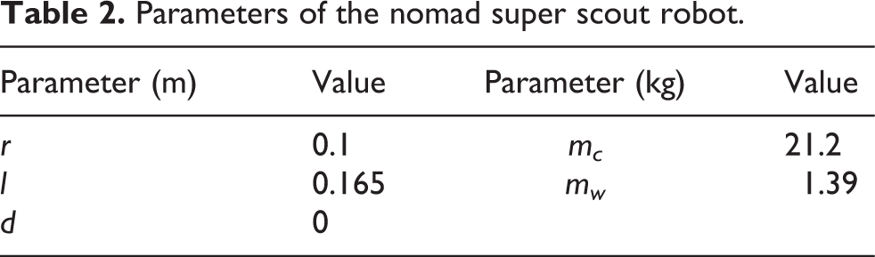
The energy consumption model was implemented in MATLAB R2013a/Simulink. The dynamic parameters of the Nomad Super Scout robot given in Table 2, as well as the dynamic parameters of the DC motors of the robot given in Table 3, were used in our model.

Table 2.

Parameters of the nomad super scout robot.

Parameter (m)	Value	Parameter (kg)	Value
r	0.1	m_c	21.2
l	0.165	m_w	1.39
d	0

Table 3.

Parameters of the motors of the nomad super scout robot.^a

Parameter	Value	Parameter	Value
R [ $Ω$ ]	2.74	K_v [(rad/s)/v]	0.069
$ν$ [Nm/(rad/s)]	0.0017	K_t [Nm/A]	0.069

^a Reference: PITTMAN GM14900.

For the validation of the proposed energy model, a Nomad Super Scout mobile robot was used (Figure 2). The robot was controlled using the built-in Motorola 68332 embedded robot controller and an Orange Pi PC Plus single-board computer. Robot Operating System was used on the Orange Pi to send the desired velocities to the robot and to receive odometry values from the encoders, as well as the power values of the motors from a custom power measurement circuit. Three batteries with weights of 5.7, 2.55, and 2.25 kg were used as payloads for the robot. The batteries were fixed on top of the robot in various combinations to achieve payload weights of 2.5, 5.7, 8.25, and 10.5 kg (Figure 2).

Figure 2.

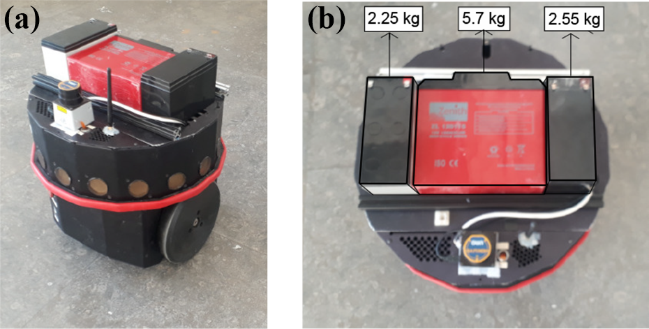
(a) Nomad Super Scout mobile robot used in this work. (b) Top view of the robot showing all the batteries that were used to vary the payload.

Calibration procedure

A calibration procedure was used to estimate the internal friction torque of the motors. The internal friction torque is related to opposing forces applied to the robot, such as the friction of the wheels with the floor and the friction in the gears. However, the load torque is related to the acceleration, mass of the robot, and the payload, and it is calculated using the dynamic robot model. Therefore, the dynamic motor model may be used for the calibration. The friction torque of the motor can be found by assuming no acceleration. In this case, the model can be written as

\begin{matrix} i (t) = b_{1} + b_{2} \dot{θ} \\ V (t) = c_{1} + c_{2} \dot{θ} \end{matrix}

where

\begin{array}{l} b_{1} = \frac{T_{m}}{K_{t} n}, b_{2} = \frac{ν}{K_{t} n} \\ c_{1} = \frac{R T_{m}}{K_{t} n}, c_{2} = \frac{R ν}{K_{t} n} + K_{v} n \end{array}

Then, the average value of the current and voltage was calculated using the power values from the measurement circuit, when the robot reaches and stays in a constant linear velocity. In the experiment, constant velocities between 0.1 m/s and 0.9 m/s were used. In Figure 3, current and voltage for a constant velocity of 0.8 m/s are shown. The shaded section representing the acceleration and deceleration of the robot are thus excluded from the calibration procedure. Finally, the energy consumed by the robot was calculated using equation (29).

Figure 3.

Calibration procedure for a constant velocity of 0.8 m/s. The robot moves in a straight path on the marble floor without payload. The acceleration and deceleration of the robot are not taken into account (shaded section): (a) odometry values from encoders (maximum velocity of 0.8 m/s) and (c) the voltage of the left motor and average value.

The experiment for the calibration procedure was performed without payload, on a marble floor, along a fixed 20 m straight path. The estimate of the friction torque is obtained using least-squares fitting. The friction torque values for the motors were found out to be 0.3728 and 0.346 Nm. In Figure 4, both the energy consumed by the robot and the energy estimated by the model are shown.

Figure 4.

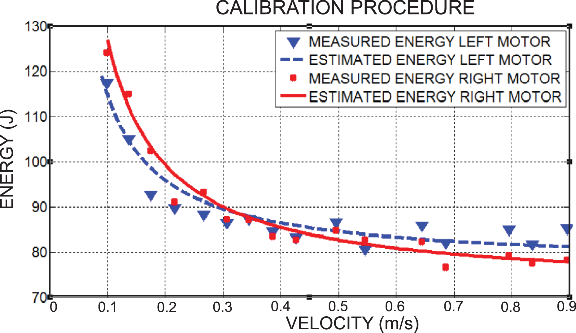
Estimated and measured energy consumption values for different velocities tested in the calibration procedure experiments.

Experimental validation of the proposed model

For the validation of the proposed power estimation model, the Nomad Super Scout mobile robot was used. A set of experiments were performed to verify the fitness of the power model for a typical mobile robot usage scenario, such as carrying various payloads or moving with different accelerations along straight and curved paths.

Straight path validation

In the experiments for the straight path validation, the mobile robot was commanded to cover a distance of 10 m, on a straight path, on a marble floor, with and without payload. A constant acceleration was applied to the robot for 4 s until it reached the desired distance, this test was repeated several times for each acceleration. The weights of the payloads were 2.55, 5.7, 8.25, and 10.5 kg, and the various accelerations were $0.125$ , $0.15$ , $0.175$ , $0.2$ , $0.225$ , and 0.25 m/s². During validation along straight paths, the angular velocity and acceleration of the wheels were the same. This behavior allows us to simplify the mathematical model into a cost function that can be used for the optimization procedure. The simplified power model depends on the angular velocity and acceleration of the wheels, as well as the payloads. The power model equation representing the experimental setup was calculated using (28) and the robot and motor parameters from Tables 2 and 3, and it is given by

\begin{matrix} P_{1} = 0.0203 {\ddot{θ}}_{1}^{2} + 0.148 {\ddot{θ}}_{1} {\dot{θ}}_{1} + 0.0014 {\ddot{θ}}_{1}^{2} m_{p} \\ + 0.102 {\ddot{θ}}_{1} + 0.0017 {\dot{θ}}_{1}^{2} + 0.005 {\ddot{θ}}_{1} {\dot{θ}}_{1} m_{p} \\ + 0.373 {\dot{θ}}_{1} + 0.0034 {\ddot{θ}}_{1} m_{p} + 0.129 \end{matrix}

\begin{matrix} P_{2} = 0.0203 {\ddot{θ}}_{2}^{2} + 0.148 {\ddot{θ}}_{2} {\dot{θ}}_{2} + 0.0014 {\ddot{θ}}_{2}^{2} m_{p} \\ + 0.0949 {\ddot{θ}}_{2} + 0.0017 {\dot{θ}}_{2}^{2} + 0.005 {\ddot{θ}}_{2} {\dot{θ}}_{2} m_{p} \\ + 0.346 {\dot{θ}}_{2} + 0.0032 {\ddot{θ}}_{2} m_{p} + 0.111 \end{matrix}

In Figure 5(a), the linear velocity profile of the mobile robot is shown. The robot develops several accelerations of 0.2 ${m/s}^{2}$ with a payload of 5.7 kg.

Figure 5.

Validation experiment, applying to the robot accelerations of 0.2 ${m/s}^{2}$ . (a) The linear velocity of the robot (odometry data) and (b) measured and estimated power values.

In Figure 5(b), the estimated and measured power of the robot generated by the accelerations are shown. It can be seen that the power estimation model predicts the average power consumed by the motor closely.

Measured and estimated energy consumptions for various accelerations are given in Table 4. The accelerations were applied to the robot, first without payload, and then with a payload of 8.25 kg. The tables show a change in the robot’s energy consumption when the accelerations of the robot increase. Comparing the tables demonstrates the energy consumption of the robot increase more when the robot carries considerable weight.

Table 4.

Measured and estimated energy consumptions with and without payload along straight paths.

Acceleration (m/s²)	Measured (J)		Estimated (J)
Acceleration (m/s²)	Left motor	Right motor	Left motor	Right motor
Energy values—without payload
0.125	56.25	53.67	60.48	57.6
0.15	58.91	56.92	60.99	58.47
0.175	60.26	56.33	63.57	60.28
0.2	61.26	57.69	64.9	62.77
0.225	60.76	56.78	66.13	64.18
0.25	61.37	57.61	65.14	64.31
Energy values—payload 8.25 kg
0.125	67.56	64.81	65.11	62.2
0.15	69	67.8	67.16	64.59
0.175	70.4	66.38	70.02	67.7
0.2	74.66	70.17	72.97	70.78
0.225	70.9	66.62	74.34	72.4
0.25	74.7	70.18	78.06	76.26

In Figure 6, the experimental results for three different accelerations and the various payloads are summarized. The figure also shows that no matter the acceleration when the payload increases, the energy consumption of the robot increases as well. The highest energy consumption of the robot happens at maximum acceleration with maximum payload (162.7 J). Figure 6 also shows that maximum acceleration with any payload can result in more energy consumption than lower accelerations with the same payload.

Figure 6.

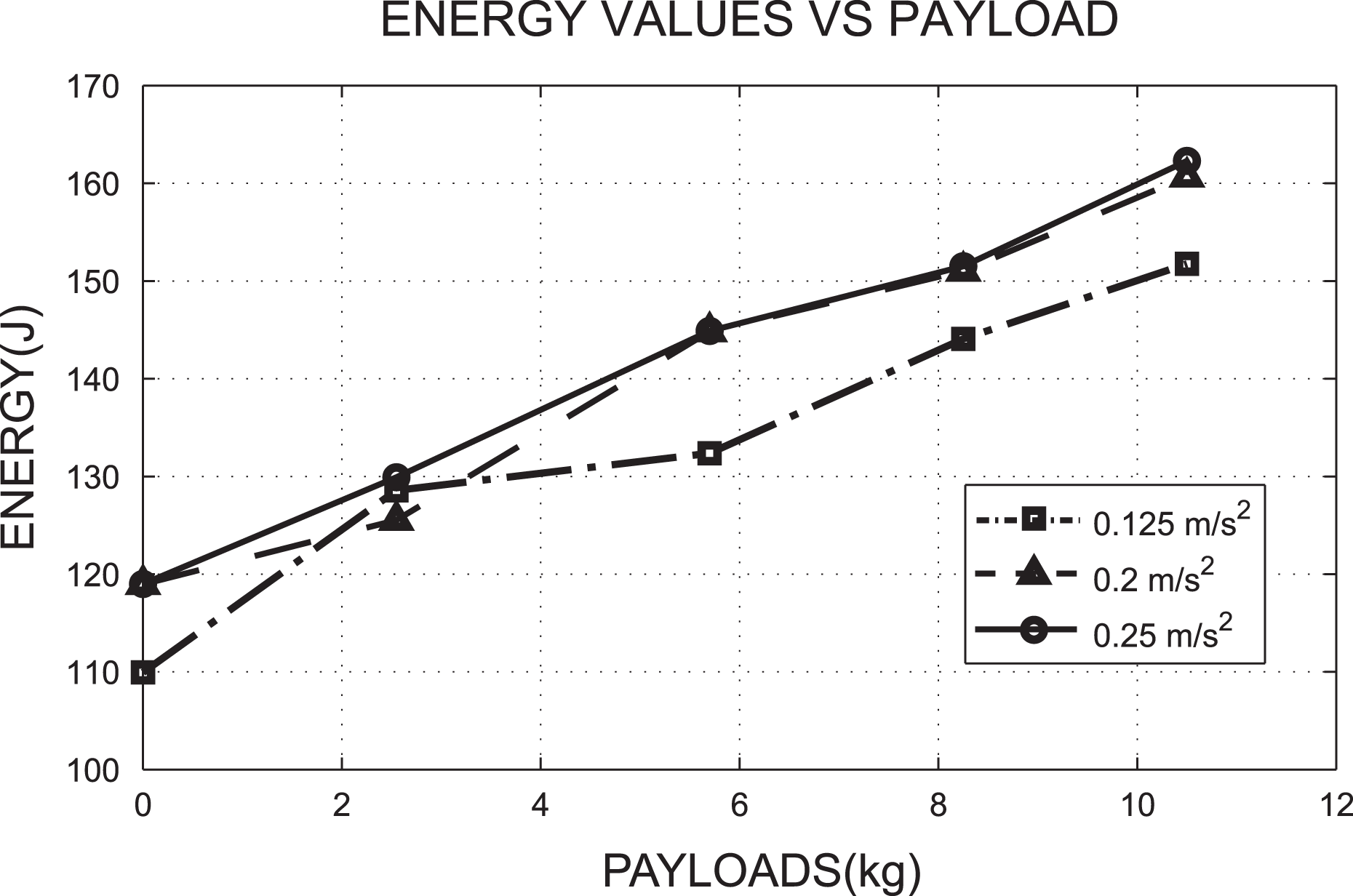
Energy consumption of the robot with different accelerations and payloads, on a straight path.

Finally, to show the fitness of the power model evaluated along straight paths, the error percentages between the measured and predicted energy values for different payloads and accelerations are given in Table 5. It is important to note that a successful result in the experiment is attained when the error between the estimated and the measured energy values is less than 10% (state-of-the-art good performance¹). The experiment with 0.225 ${m/s}^{2}$ of acceleration and without payload was the only one with a percentage higher than 10%. However, in almost all other experiments, the error is below 8%, in most cases, it is below 5%. The table shows that the best performance of the proposed model is in the middle of the set of validation accelerations for medium and high payloads.

Table 5.

Error between the predicted and measured energy.^a

Acceleration/payload (m/s²)	0 kg (%)	2.5 kg (%)	5.7 kg (%)	8.25 kg (%)	10.5 kg (%)
0.125	7.42	5.29	3.82	7.89	9.25
0.15	3.13	0.13	3.69	5.11	8.46
0.175	5.99	6.7	0.69	0.53	2.85
0.2	7.33	7.2	0.75	0.2	1.92
0.225	10.86	8.1	6.7	5.33	0.17
0.25	8.8	9.85	6.52	7.94	5.04

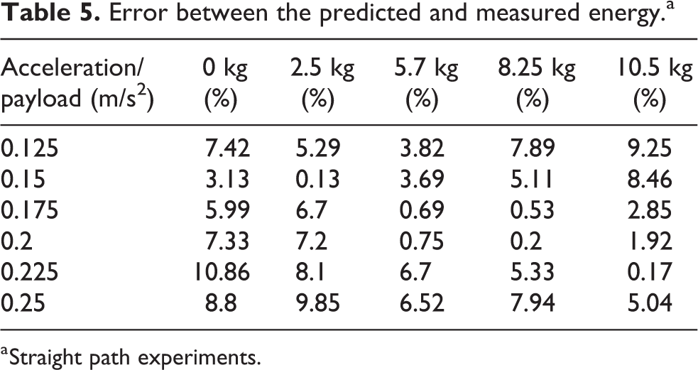
^a Straight path experiments.

In this scenario, 29 out of 30 total experiments were successful. The percentage of fitness of the predictive energy consumption compared with the robot energy consumption can be calculated with the equation (33).

Fitness (%) = \frac{Number of successful tests}{Total number of tests} \times 100

In that case, the percentage of fitness for the experiment along the straight path was equal to 96.67%. Tests accurately validated the model.

Curved path validation

In this experiment, the fitness of the power estimation model along curved paths is evaluated. For this, the mobile robot was moved along third-order Bézier curves on a marble surface. The accelerations, payloads, and directions of the robot were varied. The payloads used were 5.7, 8.25, and 10.5 kg. The equation of the third-order Bézier curve that was used in this experiment is given by

B (t) = (1 - t)^{3} p_{0} + 3 (1 - t)^{2} t p_{1} + 3 (1 - t) t^{2} p_{2} + t^{3} p_{3}

where $B$ is the 2D Bézier curve, t is the parametric variable ( $0 < t < 1$ ), and $p_{0}, p_{1}, p_{2}, p_{3}$ are the curvature control points.

The control points were chosen taking into account the dimensions of the hall where the experiments were conducted, leading to $p_{0} = (0, 0)$ , $p_{1} = (2.7, 0)$ , $p_{2} = (2.7, 0)$ , and $p_{3} = (2.7, 2.7)$ . The robot was commanded to follow the Bézier’s curve. The linear and angular velocities of the robot were received from the encoders. In Figure 7, the linear velocity of the robot given by the odometry along a right bending Bézier’s curve with no payload can be seen.

Figure 7.

Linear and angular velocities of the robot during a Bézier curve path experiment, with an acceleration of 0.18 ${m/s}^{2}$ , the right direction, and without payload.

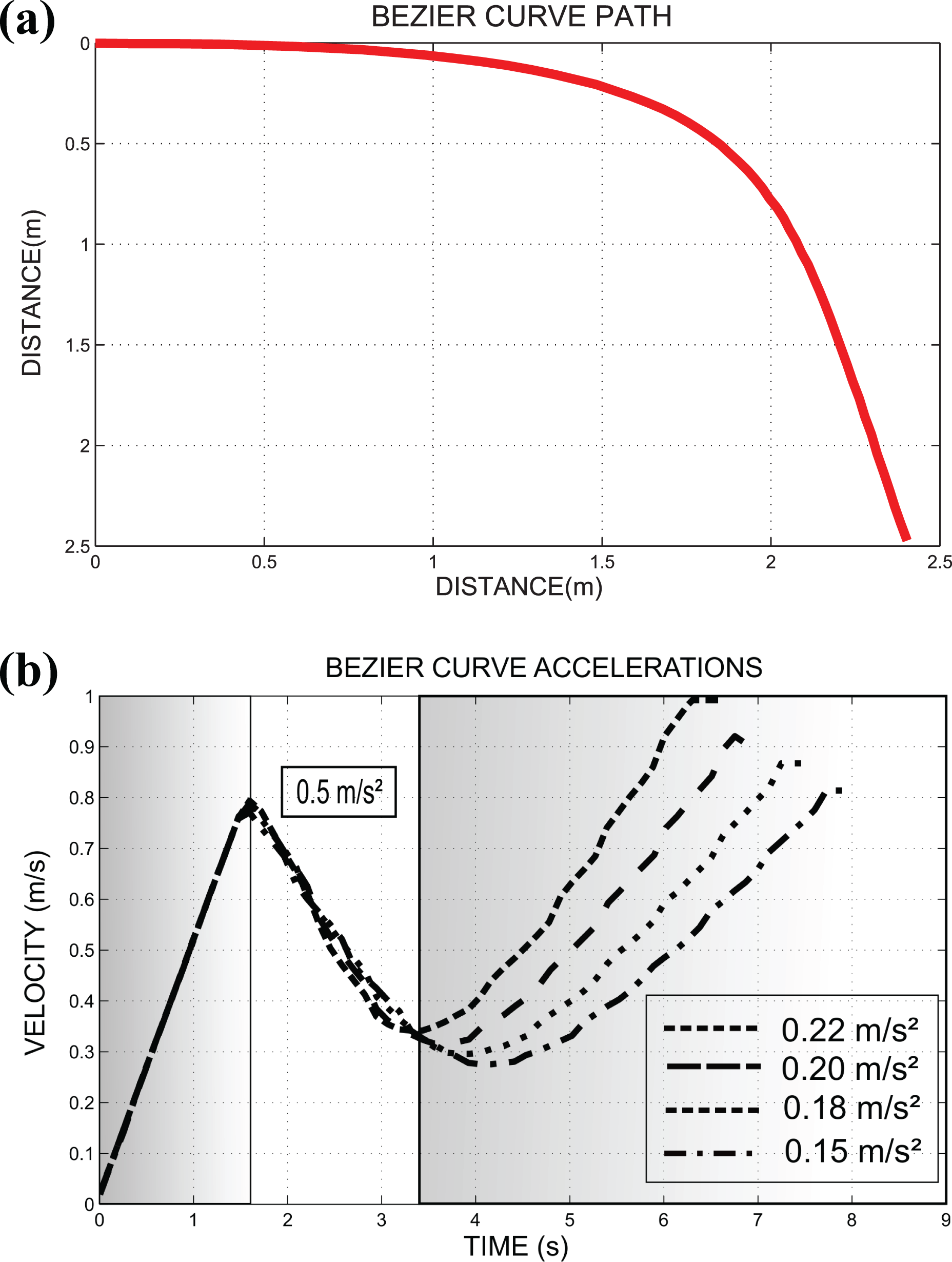
In Figure 8, the pose and linear velocities of the robot at different accelerations are shown (second shaded section) when the robot follows the Bézier curve path. The accelerations are equal to 0.15, 0.18, 0.2, and 0.22 ${m/s}^{2}$ . The first acceleration in the figure (first shaded section) corresponds to the acceleration applied by the robot controller to reach a desired maximum velocity before taking the Bézier curve path. This acceleration is equal to 0.5 ${m/s}^{2}$ .

Figure 8.

Pose and linear velocity of the robot with different accelerations. (a) Pose of the robot and (b) Bézier curve accelerations.

The odometry values given by the encoders are the linear velocity of the robot and the quaternion orientation values. But, the variables needed as the input of the proposed energy estimation model are the angular velocities of the wheels, which can be calculated with equation (35) based on the robot kinematic equations.

\begin{array}{l} {\dot{θ}}_{1} = \frac{2 v + l w}{2 r} \\ {\dot{θ}}_{2} = \frac{2 v - l w}{2 r} \end{array}

The only variable remaining is the angular velocity of the robot, which can be calculated using the quaternion orientation provided for the odometry data.

A unit quaternion can be described as

Q = [q_{w} q_{x} q_{y} q_{z}]

The quaternion can be transformed into a roll, pitch, and yaw representation, but in this case, only the yaw representation is needed (angular position of the robot $ϕ$ ). The equation that transforms the quaternion to yaw representation is shown below

ϕ = atan (\frac{2 (q_{w} q_{z} + q_{x} q_{y})}{q_{w}^{2} + q_{x}^{2} - q_{y}^{2} - q_{z}^{2}})

Finally, the angular velocity of the robot is calculated by applying the derivative of the angular position of the robot (Figure 7). Figure 9 shows the orientation of the robot and the angular velocities of the wheels calculated using the encoder values for the experiment with an acceleration of 0.15 ${m/s}^{2}$ . In this case, the angular velocities of the two wheels are different around t = 4 s, which was necessary to change the direction of the robot.

Figure 9.

Angular orientation of the robot and angular velocities of the wheels, calculated with the encoders values, for an experiment with 0.15 ${m/s}^{2}$ of acceleration. (a) Angular position of the robot and (b) the angular velocities of the wheels.

Finally, the energy consumed by the robot is estimated with the proposed power model, using the angular velocities of the wheels and different payloads as input. These estimated energy values were compared to the energy measured with the power measurement circuit on the robot.

In Figure 10, the measured and estimated power values for a no-payload experiment with 0.18 ${m/s}^{2}$ of acceleration, left direction is shown. The measured energy consumption in the left motor was 24.1 J and in the right motor 22.86 J. The estimated energy consumption in the left motor was 26.56 J and in the right motor 24.42 J, giving an error percentage of 9.26% for the left motor, 6.39% for the right motor, and 8.56% for the total.

Figure 10.

Measured and estimated power consumptions during a Bézier curve with 0.18 ${m/s}^{2}$ of acceleration, without any payload, along a Bézier curve, left direction. (a) Power of the left motor and (b) power of the right motor.

As evidenced by the data, the proposed power model overestimated the average power in the initial acceleration of the robot. This behavior emerges due to the load torque being calculated with the dynamic robot model, and this result may be overestimated as well. Nevertheless, this procedure allows the prediction of energy consumption with different accelerations and payloads.

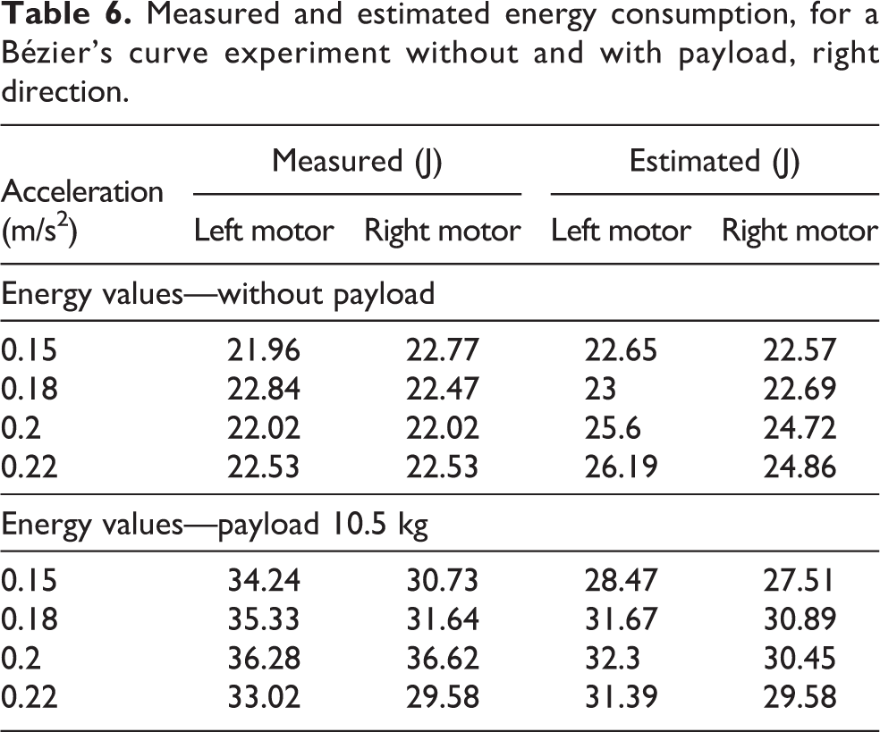
On the other hand, the overestimation behavior of the proposed model starts to decrease as the payload increases. The payload experiment result presents a better estimation in the initial acceleration of the robot, as shown in Figure 11. In the figure, the estimated power also shows an underestimated behavior at the start of the second acceleration phase. In Table 6, the measured and estimated energy consumption values of the robot are presented. The behavior of the robot along a Bézier curve is similar to its behavior along a straight path. A small change in the acceleration changes the energy consumption slightly. For example, the table shows that without payload, the difference in the energy consumed between 0.15 ${m/s}^{2}$ and 0.22 ${m/s}^{2}$ is almost 3 J for the left motor and barely change for the right. As evidenced in Table 6, substantial changes in payload cause significant changes in consumed energy. For example, a 10.5 kg payload causes the robot to consume almost 12 J more in the left motor and almost7 J more in the right.

Table 6.

Measured and estimated energy consumption, for a Bézier’s curve experiment without and with payload, right direction.

Acceleration (m/s²)	Measured (J)		Estimated (J)
Acceleration (m/s²)	Left motor	Right motor	Left motor	Right motor
Energy values—without payload
0.15	21.96	22.77	22.65	22.57
0.18	22.84	22.47	23	22.69
0.2	22.02	22.02	25.6	24.72
0.22	22.53	22.53	26.19	24.86
Energy values—payload 10.5 kg
0.15	34.24	30.73	28.47	27.51
0.18	35.33	31.64	31.67	30.89
0.2	36.28	36.62	32.3	30.45
0.22	33.02	29.58	31.39	29.58

Figure 11.

Measured and estimated power consumptions during the Bézier curve experiment, with 0.18 ${m/s}^{2}$ of acceleration, with 10.5 kg of payload, along a Bézier curve, left direction. (a) Power of the left motor and (b) power of the right motor.

In Figure 12, the behavior of the energy consumed by the robot for three accelerations and various payloads is shown. The figure also shows that the maximum energy consumption of the experiment was 66.97 J, with a medium acceleration at maximum payload. At medium payloads, the energy consumption of the robot increases as the acceleration increases.

Figure 12.

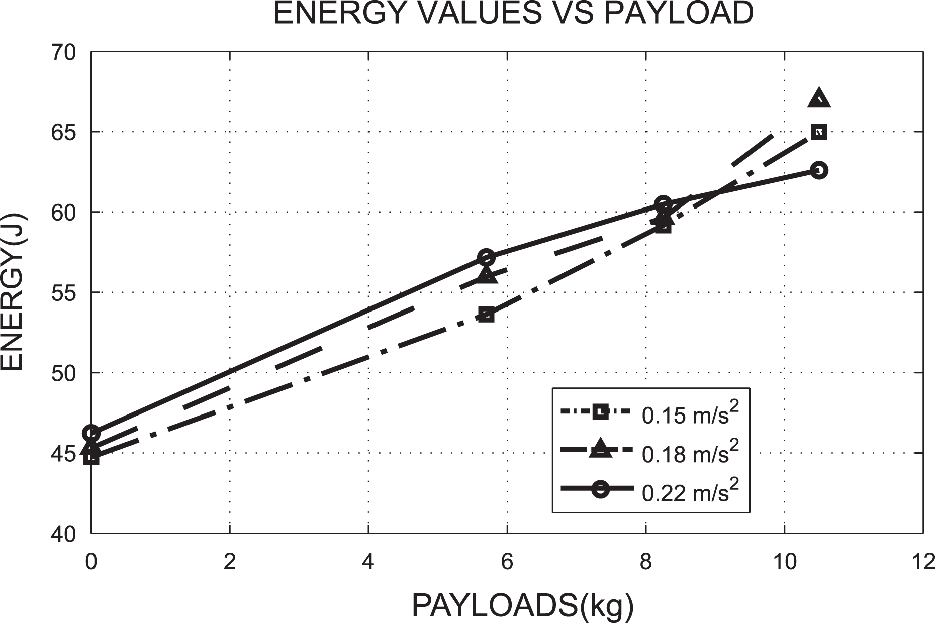
Energy consumption values of the robot with several accelerations and payloads, on the Bézier curve path.

Finally, in Table 7, the fitness of the proposed power and energy estimation model along the Bézier curve is evaluated for different accelerations and payloads. The error percentages between the measured and predicted energy consumptions in both the right and left directions are presented. Without payload and high velocities, the error percentages are significant. The table shows that the best performance of the power model is located throughout the set of validation accelerations for medium payloads. The error percentages between the predictive and measured values are below 5%. The results show that the fitness of the energy estimation model compared with the measured values given by the robot is equal to 81.25% (using equation (33)) for a Bézier curve path in both directions. The results also present that 26 out of 32 experiments accurately estimated the energy consumption of the robot.

Table 7.

The error between the predicted and measured energy, in the Bézier curve path experiment, right and left directions.

Acceleration/payload (m/s²)	0 kg (%)	5.7 kg (%)	8.25 kg (%)	10.5 kg (%)
Right direction
0.15	1.1	4.57	6.19	13.84
0.18	0.84	8.31	5.06	5.31
0.2	10.79	1.07	2.64	9.45
0.22	10.45	1.14	0.41	2.6
Left direction
0.15	6.28	1.32	8.17	14.01
0.18	8.56	1.02	4.79	8.98
0.2	13.43	0.85	3.74	8.85
0.22	13.36	2.64	0.26	5.61

Conclusion

In this article, a power and energy estimation model that takes into account robot and motor dynamic parameters was proposed. The internal friction torque of the motors was estimated using a calibration procedure. In the dynamic motor model, the load torque is directly proportional to the mass (including the payload), and the acceleration. This allows the proposed power model to predict the power and energy consumption for different payloads and accelerations, along straight and curved paths. Thanks to this model, the amount of energy a mobile robot must carry to complete a predefined task can be estimated before deployment and deviations in the predefined estimate due to unexpected changes in the payload can be estimated in real time. This allows charge optimization and scheduling not only for a single load-carrying robot but also for multiple load-carrying robots operating in warehouses with a limited number of charge stations. Future work will concentrate on the generation of the optimal motion trajectories using the proposed model for a load-carrying warehouse robot in typical operating scenarios.

The proposed model was experimentally validated using a balanced two-wheel differential drive mobile robot, the Nomad Super Scout. The results show that when the accelerations of the robot increase, the consumed energy increases. Similarly, increasing the payload increases the consumed energy as well. The fitness of the predictive power and energy estimation model compared with the energy consumed by the robot was equal to 81.25% for the Bézier curve path experiments and 96.67% for the straight path experiments. The straight path results suggest that the simplification carried out in the model is still valid, and the resulting expressions represent the dynamic behavior of the actual system. For future work, it will be interesting to evaluate the fitness of the proposed model when the center of mass of the robot is displaced considerably.

Footnotes

Declaration of conflicting interests

The author(s) declared no potential conflicts of interest with respect to the research, authorship, and/or publication of this article.

Funding

The author(s) disclosed receipt of the following financial support for the research, authorship, and/or publication of this article: This work was financially supported by Colciencias Colombia, National Scholarship—567, and partially supported by ISR—University of Coimbra, project UID/EEA/00048/2013 funded by FCT—Fundação para a Ciência e a tecnologia.

ORCID iD

Mauricio F Jaramillo-Morales

Lino Marques

References

Dogru

Marques

. Improved coverage path planning using a virtual sensor footprint: a case study on demining. In: 2019 International conference on robotics and automation (ICRA), Montreal, QC, Canada, 20–24 May 2019, pp. 4410–4415. Piscataway, New Jersey: IEEE.

Costello

Davies

Strickland

, et al. A modular mobile robotic system for cooperative payload manipulation. In: 2016 IEEE international conference on automation science and engineering (CASE), Fort Worth, TX, USA, 21–25 August 2016, pp. 573–578. Piscataway, New Jersey: IEEE.

Schlingloff

Specification and verification of collaborative transport robots. In: 2018 4th International workshop on emerging ideas and trends in the engineering of cyber-physical systems (EITEC), Porto, Portugal, 11 April 2018, pp. 3–8. Washington, D.C: IEEE computer society.

Nicholls

Strengers

. Robotic vacuum cleaners save energy? Raising cleanliness conventions and energy demand in Australian households with smart home technologies. Energy Res Soc Sci 2019; 50: 73–81.

Hendriks

Meerbeek

Boess

, et al. Robot vacuum cleaner personality and behavior. Int J Soc Robot 2011; 3(2): 187–195.

Gonzalez-de Santos

Ribeiro

Fernandez-Quintanilla

, et al. Fleets of robots for environmentally-safe pest control in agriculture. Precis Agric 2017; 18(4): 574–614.

Hameed

. Intelligent coverage path planning for agricultural robots and autonomous machines on three-dimensional terrain. J Intell Robot Syst 2014; 74(3–4): 965–983.

Chuy

Collins

, et al. Power modeling of a skid steered wheeled robotic ground vehicle. In: 2009 IEEE international conference on robotics and automation, Kobe, Japan, 12–17 May 2009, pp. 4118–4123. Piscataway, New Jersey: IEEE.

Morales

Martinez

Mandow

, et al. Power consumption modeling of skid-steer tracked mobile robots on rigid terrain. IEEE Trans Robot 2009; 25(5): 1098–1108.

10.

Chuy

Collins

JEG

, et al. Analysis and experimental verification for dynamic modeling of a skid-steered wheeled vehicle. IEEE Trans Robot 2010; 26(2): 340–353.

11.

Dogru

Marques

. A physics-based power model for skid-steered wheeled mobile robots. IEEE Trans Robot 2018; 34(2): 421–433.

12.

Kim

. Minimum-energy rotational trajectory planning for differential-driven wheeled mobile robot. In: Proceeding 13th international conference on advanced robotics, Jeju, Korea, 21–24 August 2007, pp. 265–270. Slavka: InTech.

13.

Kim

. Minimum-energy motion planning for differential-driven wheeled mobile robots. Mobile Robot Motion Plan New Challeng 2008; 2008: 193–226.

14.

Xie

Henkel

Stol

, et al. Power-minimization and energy-reduction autonomous navigation of an omnidirectional Mecanum robot via the dynamic window approach local trajectory planning. Int J Adv Robot Syst 2018; 15(1). DOI: 1729881418754563.

15.

Tokekar

Karnad

Isler

. Energy-optimal trajectory planning for car-like robots. Auton Robot 2014; 37(3): 279–300.

16.

Mei

, et al. Energy-efficient motion planning for mobile robots. In: IEEE international conference on robotics and automation, 2004. Proceedings. ICRA’04, vol. 5, New Orleans, LA, USA, 26 April–1 May 2004, pp. 4344–4349. Piscataway, New Jersey: IEEE.

17.

Mei

, et al. A case study of mobile robot’s energy consumption and conservation techniques. In: ICAR’05. Proceedings. 12th International conference on advanced robotics, Seattle, WA, USA, 18–20 July 2005, pp. 492–497. Piscataway, New Jersey: IEEE Operations Service.

18.

Parasuraman

Kershaw

Pagala

, et al. Model based on-line energy prediction system for semi-autonomous mobile robots. In: 2014 5th International conference on intelligent systems, modelling and simulation, Langkawi, Malaysia, 27–29 January 2014, pp. 411–416. Piscataway, New Jersey: IEEE.

19.

Yun

Yamamoto

. Internal dynamics of a wheeled mobile robot. In: Proceedings of 1993 IEEE/RSJ international conference on intelligent robots and systems (IROS’93), vol. 2, Yokohama, Japan, 26–30 July 1993, pp. 1288–1294. Piscataway, New Jersey: IEEE.

20.

Jaramillo-Morales

Dogru

Marques

, et al. Predictive power estimation for a differential drive mobile robot based on motor and robot dynamic models. In: 2019 Third IEEE international conference on robotic computing (IRC), Naples, Italy, 25–27 February 2019, pp. 301–307. Piscataway, New Jersey: IEEE.

21.

Yamamoto

Yun

. Coordinating locomotion and manipulation of a mobile manipulator. In: 1992 Proceedings of the 31st IEEE conference on decision and control, Tucson, AZ, USA, 16–18 December 1992, pp. 2643–2648. New York: IEEE Control Systems Society.

22.

Gholipour

Yazdanpanah

. Dynamic tracking control of nonholonomic mobile robot with model reference adaptation for uncertain parameters. In: 2003 European control conference (ECC), Cambridge, UK, 1–4 September 2003, pp. 3118–3122. Piscataway, New Jersey: IEEE.

23.

Stuart

. DC motors, speed controls, servo systems: an engineering handbook. Amsterdam: Elsevier, 2013.

Energy estimation for differential drive mobile robots on straight and rotational trajectories

Abstract

Keywords

Introduction

Development of the power model

Constraint equations

Dynamic model of the robot

Dynamic model of the motor

The combination of the dynamic models

Energy consumption model

Experiments and discussions

Experimental setup

Calibration procedure

Experimental validation of the proposed model

Straight path validation

Curved path validation

Conclusion

Footnotes

Declaration of conflicting interests

Funding

ORCID iD

References