Sage Journals: Discover world-class research

Abstract

Because wheeled mobile robots have so many applications in warehouse logistics, improving their ability to adapt to the environment has been the subject of extensive research. To enhance the traffic and obstacle avoidance capabilities of wheeled robots, a wheeled mobile robot with a transformable chassis is proposed in this article for use in an automated warehouse. The robot can not only move in all directions but also change its chassis structure according to the specific warehouse environment. First, the robot structure is designed, and the motion modes of the robot are analyzed. After kinematics analysis is performed, a kinematics model is presented. In addition, with the goal of trajectory tracking and indoor positioning, a sliding mode controller and an extended Kalman filter controller are designed. Then, the effectiveness of the kinematics model and the controller design is verified by computer simulation. Finally, a physical prototype of the robot is built and the effectiveness of the robot is demonstrated through experiments.

Keywords

Variable structure robot kinematics model trajectory tracking sliding mode controller indoor positioning

Introduction

In recent years, logistics robots are applied widely in the automated warehouses to make the transport of goods more efficiently.¹ Therefore, in the context of increasing demand for transportation robots, innovative improvement of their structural characteristics is a key focus of current research. In order to improve the maneuverability of robots, researchers have recently proposed a variety of robots, including one kind of robot that relies only on its wheels to realize its mobility. In 2019, Li et al.² designed a master–slave parallel intelligent mobile robot for the autonomous transportation of pallets in the factory logistics. The mobile robot is a combination of two sub-robots with no physical connection. Ren et al.³ proposed a state observer for friction compensation of a three-wheeled omnidirectional mobile robot (OMRs). OMRs have higher maneuverability than nonholonomic mobile robots. Tun et al.⁴ presented a reconfigurable robot, called hTetro, with a four-wheel independently controlled steering and driving mechanism to achieve the desired maneuverability for cleaning robots. Boubezoula et al.⁵ proposed an accurate and robust trajectory tracking method for a differentially driven wheeled mobile robot. Shang et al.⁶ designed a new wheel-tracked locomotion system to perform exploration tasks. To enhance the payload carrying capacity of single-platform wheeled robots, Alipour et al.⁷ proposed a tractor–trailer wheeled mobile robot that has an additional wheeled platform connected to the active platform. Sun et al.⁸ proposed a new type of transformable wheel-legged mobile robot that could be used on both flat and rugged terrains. Its wheel-legged mechanism is actually a transformable wheel. Rout et al.⁹ designed a six-wheeled mobile robot.

In summary, the existing wheeled mobile robots differ in three primary ways: by the number of wheels, the type of wheels, and the layout of the wheels. What these robots have in common is that the shape and size of the robot chassis are not transformable.

Most of the research is focused on the robots with a chassis of constant shape and size. The chassis area of that kind of robot remains constant. One of the few wheeled robots that can adjust the shape and size of their chassis is the wheel-legged robot. For a robot with a constant chassis, it is difficult to pass through a narrow width, or maneuver in a complex environment. It is obvious that a robot with a constant chassis lacks adaptation to the unstructured environment to access and perform the tasks. Luo et al.¹⁰ presented the design and development of a novel reconfigurable hybrid wheel-tracked mobile robot that can provide three locomotion modes—wheel mode, tracked mode, and climbing and rollover mode—through structure reconfiguration. A kind of robot can rely on both wheels and legs to achieve its mobility, such as a wheel-legged robot. Tadakuma et al.¹¹ proposed a new category of wheel-legged hybrid robot inspired by the retracting configuration of the armadillo. Peng et al.¹² designed the electric parallel wheel-legged robot called Bitnaza. Schwarz et al.^13,14 proposed a robot called Momaro that has four legs, with wheels on the bottom coupled to a humanoid upper torso with a head and arms. In order to improve the traveling efficiency of robots in narrow environments, a robot that can adjust its chassis size and shape is proposed in this article. This robot is able to adjust the size of its chassis within a certain degree of flexibility, similar to a wheel-legged robot. However, this robot is a pure wheeled robot with no legs. The shape and size of its chassis can be adjusted according to the environment. The area of its chassis is a variable in a certain range. Given the exact value of the robot geometric parameters, the area of the chassis can attain a maximum and a minimum value by tuning the parameters.

Many scholars have carried out research on the control of wheeled robots. Panahandeh et al.¹⁵ proposed two control strategies for the posture stabilization of a differentially driven wheeled mobile robot. Wu et al.¹⁶ eliminated the pose deviations of the mobile robot with the backstepping control technique based on the kinematic model. A trajectory controller for a four-wheel skid steering mobile robot is proposed.¹⁷ The proposed control system is based on an enhanced self-organizing incremental neural network (NN). Considering the friction dynamics in robot tracking control system, an NN-based composite learning robot control strategy with friction compensation was proposed.¹⁸ The proposed method had potential use in robot control. The feedback linearization approach is used to design a motion controller for unicycle-type wheeled mobile robots.¹⁹ The control algorithm using this feedback linearization method is presented for a wheeled mobile cable-driven parallel robot.^20,21 To avoid obstacles through the structural transformation of the robot, a perfect perception system is essential. Usually, such information cannot be collected from only one sensor. Two types of extended Kalman filters are proposed to combine the data from multiple sensors for autonomous vehicle navigation.²² Most of the research is focused on autonomy, path planning, perceptions, and control. However, tight space corners and traffic efficiency are the primary constraints of the robot with a constant chassis.

A variable structure robot is proposed in this article. A wheeled mobile robot with a transformable chassis is designed. According to kinematics analysis, a kinematics model is established. In addition, the trajectory tracking controller is presented based on sliding mode control. Moreover, research on the positioning of mobile robots in an indoor environment is carried out. The validity of the robot proposed is verified by computer simulations and experiments using a real prototype. This article makes three primary contributions to the literature.

It is the first time that a wheeled robot with a transformable chassis is presented. The shape and size of its chassis can be adjusted according to the requirements of the environment.

A kinematics model is proposed for the variable structure wheeled robot. A sliding mode controller and an extended Kalman filter algorithm are designed to achieve the goal of tracking control for the robot.

Experimental results on a real prototype robot are provided to verify the effectiveness of the proposed scheme.

Structure design

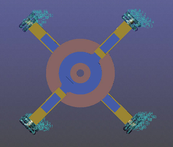
There are four omnidirectional wheels, and they are fixed on the four corners of the chassis. The chassis is built with an “X” frame. As shown in Figure 1, the robot consists of three parts. The first part is the moving mechanism, which is composed of four omnidirectional wheels. The second part is the telescopic mechanism, which consists of four linear guides and four lead screws. Screws 1 and 3 are driven with one motor, while screws 2 and 4 are driven with a second motor. The third part is the X-shaped rotary mechanism that can adjust the angle between linear guide 1 and linear guide 2. The rotary mechanism is driven by two motors mounted vertically. The conceptual design and virtual prototype of the robot are shown in Figures 1 and 2, respectively.

Figure 1.

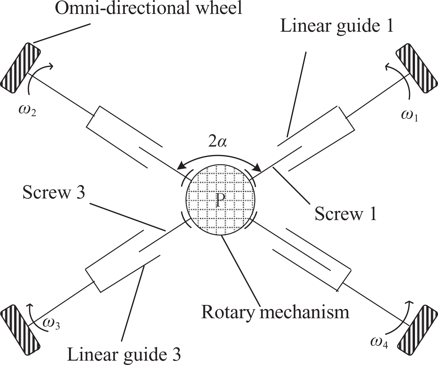
Conceptual design of the variable structure robot.

Figure 2.

Virtual prototype of the variable structure robot.

The robot proposed in this article with the novel X structure has better performance than other traditional wheeled mobile robots. Its special advantage is its transformable structure. Its flexibility is mainly reflected in two aspects. One is that it can change its width by adjusting the angle of the X-shaped mechanism $2 α$ . The other is that it can change its size by regulating the distance between two parallel wheels. In order to avoid the swinging of linear guides when the rotary mechanism driving motors are powered down, a worm gear reducer is positioned between the rotary servo motor and the gear. It can provide enough torque for the rotary mechanism. These designs will be helpful in improving the robot’s ability to adapt to the environment.

Kinematics analysis

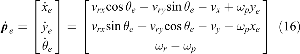
Based on the structure of this robot, the relationship between the moving velocity of the robot and the driving speed of the four wheels is analyzed, so that the kinematics model can be built.

The following assumptions are made:

Each part of the transformable structure robot is regarded as a rigid body. (The error caused by smaller bending deformation can be neglected for the reason that the robot structure will not normally have large bending deformation.)

The variable structure robot moves on a flat ground. (The motion of the robot on the flat ground is analyzed in this article, while the motion of the robot on rough terrain will be studied in the future.)

The robot’s center of mass coincides with the geometrical center of the robot. (The ideal hypothesis is to simplify the kinematics model.)

Coordinate system establishment

The coordinate system of the robot is shown in Figure 3.

Figure 3.

Kinematics coordinate system.

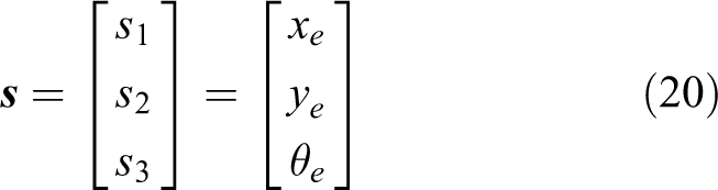
In Figure 3, ${x_{b}, y_{b}}$ is the coordinate system fixed on the ground, and ${x_{m}, y_{m}}$ is the coordinate system fixed on the robot. The origin of the robot coordinate system is set at the center of the robot (point P). Point P in the world coordinate system is (x, y), and the angle between the axis X_m and the axis X_b is θ. The counterclockwise direction is the positive direction with the X_b axis as a reference.

$p = {[\begin{matrix} x & y & θ \end{matrix}]}^{T}$ denotes the position of the robot in the world coordinate system, and $\dot{p} = {[\begin{matrix} v_{b x} & v_{b y} & ω_{b p} \end{matrix}]}^{T}$ .

$R (θ) = [\begin{matrix} cos θ & - sin θ & 0 \\ sin θ & cos θ & 0 \\ 0 & 0 & 1 \end{matrix}]$ denotes the rotation matrix. The direction of the robot coordinate system relative to the world coordinate system is described with this rotation matrix.

Kinematics formula

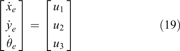
We assume that the robot has a positive direction of the Y_m axis, and the linear guides are distributed symmetrically around the X_m axis and Y_m axis. The distance between the wheel and the center of the robot is L. The angle between the linear guide and the forward direction is α. The speed of the point P is ${[\begin{matrix} v_{x} & v_{y} & ω_{p} \end{matrix}]}^{T}$ , the wheel radius is r, the angular velocity of the wheel is denoted as $ω_{i}$ (i = 1, 2, 3, 4), and the speed at which the small roller rotates is $v_{g i}$ (i = 1, 2, 3, 4). When the omnidirectional wheel rotates at a given angular velocity, it has two speeds. One is the linear velocity of the wheel along the direction perpendicular to the linear guide. The other is the speed at which the roller rotates around its own axis. Below, we use wheel 1 as an example for kinematics analysis.

(1) Taking wheel 1 as the research object, the velocity of the center of wheel 1 can be presented as

[\begin{matrix} v_{1 x} \\ v_{1 y} \end{matrix}] = [\begin{matrix} - r cos α & sin α \\ r sin α & cos α \end{matrix}] [\begin{matrix} ω_{1} \\ v_{g 1} \end{matrix}]

(2) Taking the robot as the research object, the velocity of the center of wheel 1 can be presented as

[\begin{matrix} v_{1 x} \\ v_{1 y} \end{matrix}] = [\begin{matrix} 1 & 0 & - L cos α \\ 0 & 1 & L sin α \end{matrix}] [\begin{matrix} v_{x} \\ v_{y} \\ ω_{p} \end{matrix}]

According to equations (1) and (2), we can obtain

ω_{1} = [\begin{matrix} - cos α / r & sin α / r & L / r \end{matrix}] [\begin{matrix} v_{x} \\ v_{y} \\ ω_{p} \end{matrix}]

Similarly, we can analyze the velocity of wheels 2–4 and obtain

[\begin{matrix} ω_{1} \\ ω_{2} \\ ω_{3} \\ ω_{4} \end{matrix}] = [\begin{matrix} - cos α / r & sin α / r & L / r \\ cos α / r & sin α / r & - L / r \\ - cos α / r & sin α / r & - L / r \\ cos α / r & sin α / r & L / r \end{matrix}] [\begin{matrix} v_{x} \\ v_{y} \\ ω_{p} \end{matrix}]

We can see that the angular velocity of each wheel is related to the velocity of the robot in the x and y directions and the angular velocity of the robot.

Let $J = [\begin{matrix} - cos α / r & sin α / r & L / r \\ cos α / r & sin α / r & - L / r \\ - cos α / r & sin α / r & - L / r \\ cos α / r & sin α / r & L / r \end{matrix}]$ . The angle α in the coefficient matrix is an acute angle, and both L and r are larger than zero. Moreover, rank( J ) is always equal to 3. Therefore, the robot can move in all directions on the plane.

To describe the motion of the robot more clearly, it is necessary to establish the corresponding velocity in the world coordinate system. Assuming that the velocity of the robot in the robot coordinate system is ${[\begin{matrix} v_{x} & v_{y} & ω_{p} \end{matrix}]}^{T}$ , the velocity in the world coordinate system is ${[\begin{matrix} v_{b x} & v_{b y} & ω_{b p} \end{matrix}]}^{T}$ ; then

[\begin{matrix} v_{b x} \\ v_{b y} \\ ω_{b p} \end{matrix}] = [\begin{matrix} cos θ & - sin θ & 0 \\ sin θ & cos θ & 0 \\ 0 & 0 & 1 \end{matrix}] [\begin{matrix} v_{x} \\ v_{y} \\ ω_{p} \end{matrix}]

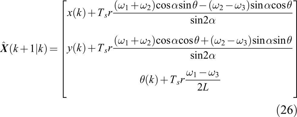
Therefore, the kinematics model of the robot in the world coordinate system is as follows

[\begin{matrix} ω_{1} \\ ω_{2} \\ ω_{3} \\ ω_{4} \end{matrix}] = J R^{- 1} (θ) [\begin{matrix} v_{b x} \\ v_{b y} \\ ω_{b p} \end{matrix}]

Substituting J and $R^{- 1} (θ)$ into equation (6), we get

[\begin{matrix} ω_{1} \\ ω_{2} \\ ω_{3} \\ ω_{4} \end{matrix}] = [\begin{matrix} - cos (θ - α) / r & - sin (θ - α) / r & L / r \\ cos (θ + α) / r & sin (θ + α) / r & - L / r \\ - cos (θ - α) / r & - sin (θ - α) / r & - L / r \\ cos (θ + α) / r & sin (θ + α) / r & L / r \end{matrix}] [\begin{matrix} v_{b x} \\ v_{b y} \\ ω_{b p} \end{matrix}]

From equation (7), we can obtain the relationship between the angular velocity of each wheel and the velocity of the robot in the world coordinate system.

However, when the angular velocities of the four wheels are known, and the motion state of the mobile robot is needed, it is necessary to obtain the inverse solution of equation (4). In the case of a constant structure, angle α is constant. At this time, equation (4) is a non-homogeneous linear equation system, and the augmented matrix can be expressed by the row transformation as follows

[\begin{matrix} - cos α / r & sin α / r & L / r & ω_{1} \\ 0 & 2 sin α / r & 0 & ω_{1} + ω_{2} \\ 0 & 0 & - 2 L / r & ω_{3} - ω_{1} \\ 0 & 0 & 0 & - ω_{1} - ω_{2} + ω_{3} + ω_{4} \end{matrix}]

The necessary and sufficient condition for the solution of the non-homogeneous linear equations is that the rank of the coefficient matrix is equal to the rank of the augmented matrix. Therefore, the inverse solution is

{\begin{cases} v_{x} = (ω_{2} - ω_{3}) r / (2 cos α) \\ v_{y} = (ω_{1} + ω_{2}) r / (2 sin α) \\ ω_{p} = (ω_{1} - ω_{3}) r / (2 L) \end{cases}

At the same time, the above equations must satisfy $- ω_{1} - ω_{2} + ω_{3} + ω_{4} = 0$ ; otherwise, there is no solution.

Similarly, the inverse solution of equation (7) can be obtained

{\begin{cases} v_{b x} = \frac{(ω_{1} + ω_{2}) r cos α sin θ - (ω_{2} - ω_{3}) r sin α cos θ}{sin 2 α} \\ v_{b y} = \frac{(ω_{1} + ω_{2}) r cos α cos θ + (ω_{2} - ω_{3}) r sin α sin θ}{sin 2 α} \\ ω_{b p} = \frac{(ω_{1} - ω_{3}) r}{2 L} \end{cases}

At the same time, the above equations must satisfy $- ω_{1} - ω_{2} + ω_{3} + ω_{4} = 0$ .

Special forms of movement

Based on the kinematics model of the robot, the common motion states of the robot are analyzed. They are as follows.

(1) In situ rotation

When $v_{x} = 0, v_{y} = 0, ω_{p} \neq 0$ , the center coordinates of the robot are constant, and the robot rotates around the center at a constant angular velocity $ω_{p}$ . An initial value is substituted into equation (4), and we can obtain

ω_{1} = ω_{4} = - ω_{2} = - ω_{3} = ω_{p} L / r

The robot can realize rotation at the angular velocity $ω_{p}$ .

(2) Rectilinear motion in the x or y direction

When $v_{x} \neq 0, v_{y} = 0, ω_{p} = 0$ , the center point of the robot has rectilinear motion along the coordinate axis at a certain velocity. An initial value is substituted into equation (4), and we can obtain

ω_{1} = - ω_{2} = ω_{3} = - ω_{4} = - v_{x} cos α / r

The robot can have rectilinear motion in the x direction.

Similarly, when $v_{x} = 0, v_{y} \neq 0, ω_{p} = 0$ , and substituting values into equation (4), we can obtain

ω_{1} = ω_{2} = ω_{3} = ω_{4} = v_{y} sin α / r

The robot can have rectilinear motion in the y direction.

(3) Motion at a certain heading angle

When $v_{x} \neq 0, v_{y} \neq 0, ω_{p} = 0$ , the center point of the robot moves along a certain line in the coordinate system at a certain velocity. An initial velocity value is substituted into equation (4), and we can obtain

{\begin{cases} ω_{1} = ω_{3} = (- v_{x} cos α + v_{y} sin α) / r \\ ω_{2} = ω_{4} = (v_{x} cos α + v_{y} sin α) / r \end{cases}

The robot can have rectilinear motion at a certain heading angle. The angle between the motion trajectory and the coordinate axis is related to v_x and v_y .

Controller design

This section describes the design of a trajectory tracking controller and a robot positioning controller for the variable structure robot.

Trajectory tracking controller design

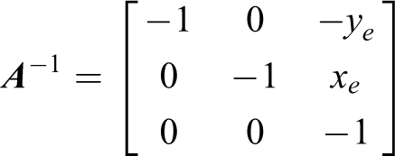
Mathematical model of trajectory tracking

From the previous kinematics analysis, the kinematics model of the mobile robot designed in this article can be described as follows

\dot{p} = [\begin{matrix} \dot{x} \\ \dot{y} \\ \dot{θ} \end{matrix}] = [\begin{matrix} cos θ & - sin θ & 0 \\ sin θ & cos θ & 0 \\ 0 & 0 & 1 \end{matrix}] [\begin{matrix} v_{x} \\ v_{y} \\ ω_{p} \end{matrix}] = R (θ) q

$p = {[\begin{matrix} x & y & θ \end{matrix}]}^{T}$ is the current pose of the robot in the world coordinate system. $q = {[\begin{matrix} v_{x} & v_{y} & ω_{p} \end{matrix}]}^{T}$ is the input control variable for the robot. v_x and v_y are the speeds of the robot along the x and y axes in the robot coordinate system, respectively. $ω_{p}$ is the rotational angular velocity of the robot.

The desired input of the robot is defined as $q_{r} = {[\begin{matrix} v_{r x} & v_{r y} & ω_{r} \end{matrix}]}^{T}$ , and the desired pose of the robot in the world coordinate system is defined as $p_{r} = {[\begin{matrix} x_{r} & y_{r} & θ_{r} \end{matrix}]}^{T}$ . The error vector of the robot pose is defined as $p_{e} = {[\begin{matrix} x_{e} & y_{e} & θ_{e} \end{matrix}]}^{T}$ . The error vector is transformed from the world coordinate system into the robot coordinate system ${x_{m}, y_{m}}$ of the current pose, and then the pose error equation can be expressed as

p_{e} = [\begin{matrix} x_{e} \\ y_{e} \\ θ_{e} \end{matrix}] = R^{- 1} (θ) [\begin{matrix} x_{r} - x \\ y_{r} - y \\ θ_{r} - θ \end{matrix}] = [\begin{matrix} cos θ & sin θ & 0 \\ - sin θ & cos θ & 0 \\ 0 & 0 & 1 \end{matrix}] [\begin{matrix} x_{r} - x \\ y_{r} - y \\ θ_{r} - θ \end{matrix}]

By performing a differential operation on equation (15), we obtain

{\dot{p}}_{e} = [\begin{matrix} {\dot{x}}_{e} \\ {\dot{y}}_{e} \\ {\dot{θ}}_{e} \end{matrix}] = [\begin{matrix} v_{r x} cos θ_{e} - v_{r y} sin θ_{e} - v_{x} + ω_{p} y_{e} \\ v_{r x} sin θ_{e} + v_{r y} cos θ_{e} - v_{y} - ω_{p} x_{e} \\ ω_{r} - ω_{p} \end{matrix}]

That is

[\begin{matrix} {\dot{x}}_{e} \\ {\dot{y}}_{e} \\ {\dot{θ}}_{e} \end{matrix}] = [\begin{matrix} - 1 & 0 & y_{e} \\ 0 & - 1 & - x_{e} \\ 0 & 0 & - 1 \end{matrix}] [\begin{matrix} v_{x} \\ v_{y} \\ ω_{p} \end{matrix}] + [\begin{matrix} v_{r x} cos θ_{e} - v_{r y} sin θ_{e} \\ v_{r x} sin θ_{e} + v_{r y} cos θ_{e} \\ ω_{r} \end{matrix}]

It can be seen from equation (17) that the model is a multi-input nonlinear coupling system. We can decouple it as follows.

First of all, let $A = [\begin{matrix} - 1 & 0 & y_{e} \\ 0 & - 1 & - x_{e} \\ 0 & 0 & - 1 \end{matrix}]$ , and $| A | = - 1$ . Therefore, A is always reversible.

Then, the decoupling algorithm is designed as follows

[\begin{matrix} v_{x} \\ v_{y} \\ ω_{p} \end{matrix}] = A^{- 1} [\begin{matrix} u_{1} - v_{r x} cos θ_{e} + v_{r y} sin θ_{e} \\ u_{2} - v_{r x} sin θ_{e} - v_{r y} cos θ_{e} \\ u_{3} - ω_{r} \end{matrix}]

Here, u ₁, u ₂, and u ₃ are the control variables to be designed.

A^{- 1} = [\begin{matrix} - 1 & 0 & - y_{e} \\ 0 & - 1 & x_{e} \\ 0 & 0 & - 1 \end{matrix}]

By substituting equation (18) into equation (17), we get the following expression

[\begin{matrix} {\dot{x}}_{e} \\ {\dot{y}}_{e} \\ {\dot{θ}}_{e} \end{matrix}] = [\begin{matrix} u_{1} \\ u_{2} \\ u_{3} \end{matrix}]

Sliding mode controller design

According to the above analysis, the trajectory tracking problem of robots can be transformed into the stabilization problem of the error system.

Because the robot studied in this article has omnidirectional mobility, the velocity value of the variable structure mobile robot should be described as along the x-direction, along the y-direction, and at the angular velocity of the rotation. Therefore, this article designs three sliding mode surfaces, which track x, y, and θ, respectively. The sliding mode surface function is designed as follows

s = [\begin{matrix} s_{1} \\ s_{2} \\ s_{3} \end{matrix}] = [\begin{matrix} x_{e} \\ y_{e} \\ θ_{e} \end{matrix}]

For the sliding mode control, we use the approach law and then obtain

\dot{s} = - K s - Γ sgn (s)

Here, $K =dia g (k_{1}, k_{2}, k_{3})$ , $Γ =dia g (δ_{1}, δ_{2}, δ_{3})$ , and $k_{1}, k_{2}, k_{3}, δ_{1}, δ_{2}, δ_{3}$ are positive parameters.

Let

[\begin{matrix} u_{1} \\ u_{2} \\ u_{3} \end{matrix}] = [\begin{matrix} {\dot{s}}_{1} \\ {\dot{s}}_{2} \\ {\dot{s}}_{3} \end{matrix}] = [\begin{matrix} - k_{1} s_{1} - δ_{1} sgn (s_{1}) \\ - k_{2} s_{2} - δ_{2} sgn (s_{2}) \\ - k_{3} s_{3} - δ_{3} sgn (s_{3}) \end{matrix}]

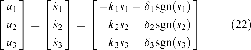
According to equations (18) and (22), the sliding mode control law can be designed as follows

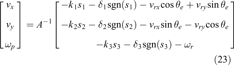
[\begin{matrix} v_{x} \\ v_{y} \\ ω_{p} \end{matrix}] = A^{- 1} [\begin{matrix} - k_{1} s_{1} - δ_{1} sgn (s_{1}) - v_{r x} cos θ_{e} + v_{r y} sin θ_{e} \\ - k_{2} s_{2} - δ_{2} sgn (s_{2}) - v_{r x} sin θ_{e} - v_{r y} cos θ_{e} \\ - k_{3} s_{3} - δ_{3} sgn (s_{3}) - ω_{r} \end{matrix}]

Calculating and simplifying equation (23) yields

\begin{matrix} v_{x} = & k_{1} s_{1} + δ_{1} sgn (s_{1}) + (ω_{r} + k_{3} s_{3} + δ_{3} sgn (s_{3})) y_{e} + v_{r x} cos θ_{e} - v_{r y} sin θ_{e} \\ v_{y} = & k_{2} s_{2} + δ_{2} sgn (s_{2}) - (ω_{r} + k_{3} s_{3} + δ_{3} sgn (s_{3})) x_{e} + v_{r x} sin θ_{e} + v_{r y} cos θ_{e} \\ ω_{p} = & ω_{r} + k_{3} s_{3} + δ_{3} sgn (s_{3}) \end{matrix}

After designing the sliding mode controller for the trajectory tracking for the robot, further stability analysis of the control system is proposed.

The Lyapunov function is

V_{1} = \frac{1}{2} s_{1}^{2} = \frac{1}{2} x_{e}^{2}

Then,

{\dot{V}}_{1} = s_{1} {\dot{s}}_{1} = - k_{1} s_{1}^{2} - δ_{1} | s_{1} | \leq - k_{1} s_{1}^{2} .

Similarly, the Lyapunov functions are taken for y_e and $θ_{e}$ . Then, ${\dot{V}}_{2} = s_{2} {\dot{s}}_{2} \leq - k_{2} s_{2}^{2}$ and ${\dot{V}}_{3} = s_{3} {\dot{s}}_{3} \leq - k_{3} s_{3}^{2}$ .

Therefore, the system satisfies the condition ${\dot{V}}_{i} = s_{i} {\dot{s}}_{i} \leq 0$ (i = 1, 2, 3). Under the action of the sliding mode controller, the system states can reach the sliding mode surface $s = 0$ in a limited time, that is, $x_{e} = y_{e} = θ_{e} = 0$ is the global asymptotically stable equilibrium point of the system.

Positioning controller design

The positioning controller is designed for the robot based on the extended Kalman filter algorithm.

Establishment and analysis of discrete models

(1) Discrete kinematics model of the robot

We assume that the state variable of the robot is $\hat{X} (k | k) = {[x (k), y (k), θ (k)]}^{T}$ .

The sampling time is T_s , we discretize equation (9), and we obtain the prior state estimate $\hat{X} (k + 1 | k)$

\hat{X} (k + 1 | k) = f (\hat{X} (k | k)) = [\begin{matrix} x (k) + v_{b x} (k) T_{s} \\ y (k) + v_{b y} (k) T_{s} \\ θ (k) + ω_{b p} (k) T_{s} \end{matrix}]

Then

\hat{X} (k + 1 | k) = [\begin{matrix} x (k) + T_{s} r \frac{(ω_{1} + ω_{2}) cos α sin θ - (ω_{2} - ω_{3}) sin α cos θ}{sin 2 α} \\ y (k) + T_{s} r \frac{(ω_{1} + ω_{2}) cos α cos θ + (ω_{2} - ω_{3}) sin α sin θ}{sin 2 α} \\ θ (k) + T_{s} r \frac{ω_{1} - ω_{3}}{2 L} \end{matrix}]

Next, the nonlinear model is locally linearized.

A priori estimate covariance matrix is $P (k + 1 | k)$

P (k + 1 | k) = Φ (k | k) P (k | k) Φ^{T} (k | k) + Q (k)

Here, $Φ (k | k)$ is the Jacobian matrix of $f (\hat{X} (k | k))$ and $Q (k)$ is the covariance matrix of the system model noise.

Then

Φ (k + 1) = \frac{\partial f}{\partial X} = [\begin{matrix} 1 & 0 & T_{s} r \frac{(ω_{1} + ω_{2}) cos α cos θ + (ω_{2} - ω_{3}) sin α sin θ}{sin 2 α} \\ 0 & 1 & - T_{s} r \frac{(ω_{1} + ω_{2}) cos α sin θ - (ω_{2} - ω_{3}) sin α cos θ}{sin 2 α} \\ 0 & 0 & 1 \end{matrix}]

(2) Discrete model of electronic compass

In order to observe the azimuth information of the mobile robot in the world coordinate system, an electronic compass is used to collect the data of the mobile robot. Its observation model can be described as

γ = arctan \frac{y}{x} + μ

Here, γ is the azimuth of the robot in the world coordinate system measured by the electronic compass. x and y represent the position of the robot in the world coordinate system. μ is the Gaussian white noise error present in the electronic compass sensor.

(3) Discrete model of ultrasonic sensor

In this article, eight ultrasonic sensors are used, and their distribution is shown in Figure 4. The ultrasonic sensors are mounted on the top cover of the robot. The laser scanner is installed at the geometric center of the mobile robot and the electronic compass is mounted directly under the lidar.

Figure 4.

Layout of multiple sensors on the robot.

According to the ultrasonic modeling method for mobile robot obstacle avoidance and path planning based on multi-sensor information fusion,^23,24 the coordinate system of the ultrasonic sensor is shown in Figure 5. We assume that the position of the ith ultrasonic sensor in the robot coordinate system is $(x_{m i}, y_{m i})$ , and the angle between the central axis of the ultrasonic sensor and the angle between the central axis of the ultrasonic sensor and the x_m -axis is $γ_{m i}$ . The angle of the ultrasonic wave emitted by the ultrasonic sensor is δ, and the vertical distance from the emission point of the ultrasonic sensor to the jth obstacle is d_j . We assume that the jth obstacle is shown in Figure 5. The angle between the line and the x-axis is $β_{j}$ , and the vertical distance from the obstacle to the origin is L_j . An observation model can be established as follows

\begin{array}{l} d_{j} = L_{j} - (x (k) + x_{m i} cos θ (k) - y_{m i} sin θ (k)) cos β_{j} \\ - (y (k) + x_{m i} sin θ (k) + y_{m i} cos θ (k)) sin β_{j} \end{array}

and $γ_{i} (k) - \frac{δ}{2} < β_{j} < γ_{i} (k) + \frac{δ}{2}$ .

(4) Discrete model of the lidar

Figure 5.

Coordinate diagram of the ultrasonic sensor.

According to the model for the lidar,^25,26 the coordinate system of the lidar is shown in Figure 6, where the lidar is located at point O_m of the robot coordinate system. We assume that there are two fixed points in the world coordinate system, shown as A and B in Figure 6. The distance and angle between the robot and the two fixed points can be observed with the lidar.

Figure 6.

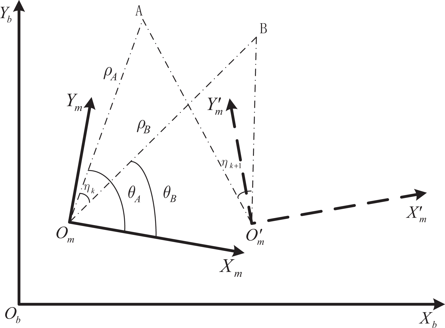
Coordinate system of the lidar.

We assume that the observation equation of the lidar is $Z_{2} (k) = cos η (k)$ . That is the cosine of the angle between the vector $O_{m} A$ and the vector $O_{m} B$ in the coordinates of the robot at that moment.

The observation model of the sensor is

cos η (k + 1) = \frac{e_{x A b} e_{x B b} + e_{y A b} e_{y B b}}{\sqrt{(e_{x A b}^{2} + e_{y A b}^{2}) (e_{x B b}^{2} + e_{y B b}^{2})}}

In which, $e_{x A b} = x (k + 1) - x_{A b}$ , $e_{x B b} = x (k + 1) - x_{B b}$ , $e_{y A b} = y (k + 1) - y_{A b}$ , and $e_{y B b} = y (k + 1) - y_{B b}$ .

The observation model of the sensor is

Z (k) = h (X (k)) + V (k)

Here, $h (X (k))$ is the observation function of each sensor, and $V (k)$ is the observation error of each sensor. We suppose that these observation errors have a zero mean Gaussian white noise error and the variance is $R (k)$ .

The observation models of the sensors are expressed as follows

\begin{array}{l} {\hat{Z}}_{1} (k + 1 | k) = arctan \frac{\hat{y} (k + 1 | k)}{\hat{x} (k + 1 | k)} \\ {\hat{Z}}_{2} (k + 1 | k) = \frac{{\hat{e}}_{x A b} {\hat{e}}_{x B b} + {\hat{e}}_{y A b} {\hat{e}}_{y B b}}{\sqrt{({\hat{e}}_{x A b}^{2} + {\hat{e}}_{y A b}^{2}) ({\hat{e}}_{x B b}^{2} + {\hat{e}}_{y B b}^{2})}} \\ {\hat{Z}}_{2+m} (k + 1 | k) = L_{j} - [x_{m i} cos \hat{θ} (k + 1 | k) - y_{m i} sin \hat{θ} (k + 1 | k) + \hat{x} (k + 1 | k)] cos β_{j} \\ - [x_{m i} sin \hat{θ} (k + 1 | k) + y_{m i} cos \hat{θ} (k + 1 | k) + \hat{y} (k + 1 | k)] sin β_{j} \end{array}

In which, ${\hat{e}}_{x A b} = x (k + 1 | k) - x_{A b}$ , ${\hat{e}}_{x B b} = x (k + 1 | k) - x_{B b}$ , ${\hat{e}}_{y A b} = y (k + 1 | k) - y_{A b}$ , and ${\hat{e}}_{y B b} = y (k + 1 | k) - y_{B b}$ .

Correction process of the extended Kalman filter

The actual observation of the robot through a variety of sensors is $Z (k + 1)$ , and the estimated value of the observation is $\hat{Z} (k + 1 | k)$ . The measured residual value $χ (k + 1 | k)$ can be expressed as

χ (k + 1 | k) = Z (k + 1) - \hat{Z} (k + 1 | k)

The residual value in equation (36) is also called a new interest and represents the difference between the predicted measured value and the actual measured value. The covariance matrix $S (k + 1 | k)$ is

S (k + 1 | k) = H (k + 1) P (k + 1 | k) H {(k + 1)}^{T} + R (k)

In the above formula, $H (k + 1)$ is the Jacobian matrix of $h (X (k + 1))$ .

H (k + 1) = \frac{\partial H (\hat{X} (k + 1 | k))}{\partial \hat{X} (k + 1 | k)}

By substituting equation (33) into equation (36), we obtain

H (k + 1) = [\begin{matrix} - \frac{y}{x^{2} + y^{2}} & \frac{x}{x^{2} + y^{2}} & 0 \\ f_{1} & f_{2} & 0 \\ - cos β_{j} & - sin β_{j} & x_{m i} sin (θ (k) - β_{j}) + y_{m i} cos (β_{j} - θ (k)) \end{matrix}]

$f_{1}, f_{2}$ can be expressed as follows:

{\begin{cases} f_{1} = \frac{2 x - x_{A b} - x_{B b}}{{(g_{1} g_{2})}^{1 / 2}} - \frac{(x - x_{A b}) g_{3}}{g_{1}^{3 / 2} g_{2}^{1 / 2}} - \frac{(x - x_{B b}) g_{3}}{g_{1}^{1 / 2} g_{2}^{3 / 2}} \\ f_{2} = \frac{2 y - y_{A b} - y_{B b}}{{(g_{1} g_{2})}^{1 / 2}} - \frac{(y - y_{A b}) g_{3}}{g_{1}^{3 / 2} g_{2}^{1 / 2}} - \frac{(y - y_{B b}) g_{3}}{g_{1}^{1 / 2} g_{2}^{3 / 2}} \end{cases}

In the above formulas, $(x_{A b}, y_{A b})$ and $(x_{B b}, y_{B b})$ are the coordinates of A and B, respectively, and the coordinates can be obtained by the observation value at the previous moment. g ₁, $g_{2}$ , and g ₃ are expressed as follows

{\begin{cases} g_{1} = {(x - x_{A b})}^{2} + {(y - y_{A b})}^{2} \\ g_{2} = {(x - x_{B b})}^{2} + {(y - y_{B b})}^{2} \\ g_{3} = (x - x_{A b}) (x - x_{B b}) + (y - y_{A b}) (y - y_{B b}) \end{cases}

The optimal Kalman gain matrix is $K (k + 1 | k)$ , and

K (k + 1 | k) = P (k + 1 | k) H {(k + 1)}^{T} S^{- 1} (k + 1 | k)

The Kalman gain in equation (38) is used to reduce the posteriori error covariance. After correcting the priori state estimate, the posterior state estimate is $\hat{X} (k + 1 | k + 1)$

\hat{X} (k + 1 | k + 1) = \hat{X} (k + 1 | k) + K (k + 1 | k) χ (k + 1 | k)

After correcting the priori estimate covariance matrix, the posterior estimation covariance matrix $P (k + 1)$ is updated as follows

P (k + 1 | k + 1) = [I - K (k + 1 | k) H (k + 1)] P (k + 1 | k)

Discussion

Remark 1

In this article, a new type of wheeled robot with a transformable chassis is proposed for the first time. It has a high rate of passage and a wide range of applications owing to its variable structure.

Remark 2

The chassises of the robots^1,3 are of fixed structure, meaning that the size of their chassis cannot be adjusted according to the requirements of the environment. That limits their scope of application. Furthermore, the robots are not suited for working in narrow environments. The variable structure wheeled robot proposed in this article can not only move in a wide environment but also perform tasks in narrow surroundings. No relevant studies about a robot with this type of variable structure characteristic have been found yet.

Remark 3

Higher control accuracy is obtained.¹⁷ However, the control algorithm proposed for the robot in this article has a lower computational complexity than the algorithm. Compared with related works,¹⁹ the control algorithm proposed has more parameters. The proposed algorithm in this article also has good control performance.

Computer simulation

Simulation of kinematics model

In order to verify the validity of the kinematics model, simulation experiments are proposed based on the Adams model. The simulation is carried out with the following parameters: L = 340 mm and α = 45°, and L = 390 mm and α = 60°. The virtual prototype built in Adams is shown in Figure 7. In Figure 7, the character marks on the right side of each wheel are the constraints added to each small roller of the wheels.

Figure 7.
Virtual prototype in Adams.

In situ rotation

When L = 340 mm and α = 45°, the angular velocities of the four wheels are shown in Table 1. The angular velocities of the wheels gradually increase from 0 to the given velocities. The angular velocity value $ω_{p}$ of the robot is plotted as shown in Figure 8.

Table 1.
The wheel velocities of the robot in situ rotation.

$ω_{1}$ $ω_{2}$ $ω_{3}$ $ω_{4}$

360 °/s −360 °/s −360 °/s 360 °/s

Figure 8.
The angular velocity of the robot in situ rotation 1.

When L = 390 mm and α = 60°, the angular velocities of the four wheels are shown in Table 1. The angular velocity $ω_{p}$ of the robot is plotted, as shown in Figure 9.

Figure 9.
The angular velocity of the robot in situ rotation 2.

Movement in the x direction

When L = 340 mm and α = 45°, the angular velocities of the four wheels are shown in Table 2. The angular velocities of the wheels gradually increase from 0 to the given value. The velocity v_x of the robot is plotted, as shown in Figure 10.

Table 2.
The wheel velocities of the robot in rectilinear motion.

$ω_{1}$ $ω_{2}$ $ω_{3}$ $ω_{4}$

−360 °/s 360 °/s −360 °/s 360 °/s

Figure 10.
The velocity of the robot in rectilinear motion 1.

When L = 390 mm and α = 60°, the angular velocities of the four wheels are shown in Table 2. The velocity of the robot moving in the x direction is plotted, as shown in Figure 11.

Figure 11.
The velocity of the robot in rectilinear motion 2.

It can be found that the theoretical results are consistent with the simulation results based on Adams. The simulation results verify the validity of both the kinematics model and the robot structure.

Simulation of trajectory tracking control

The reference inputs of the system are set as $v_{r x} = - ω_{r} sin θ_{r}, v_{r y} = ω_{r} cos θ_{r}, ω_{r} = π /10$ rad/s, and the desired trajectory in the world coordinate system can be described by the following three equations: $x_{r} = cos θ_{r}, y_{r} = sin θ_{r}, and θ_{r} = ω_{r} t$ . We let the initial pose of the mobile robot in the world coordinate system be $x (0) = 0.9$ m, $y (0) = - 0.1$ m, and $θ (0) = 0$ rad. Different controller parameters are used to obtain the best control effect.

The controller parameters are set as $k_{1} = k_{2} = k_{3} = 10,$ $δ_{1} = δ_{2} = δ_{3} = 2$ . The results of tracking the circular trajectory are shown in Figure 12.

Figure 12.
Trajectory tracking results of circular motion with the sliding mode controller 1. (a) Circular trajectory tracking. (b) Curves of the robot pose. (c) Curves of the trajectory tracking error. (d) Curves of the control variables. (e) Trajectory tracking error curves of the first 2 s.

As shown in Figure 12(a), the robot can track the trajectory from the initial position in a limited amount of time. The pose responses of the robot are shown in Figure 12(b). As shown in Figure 12(c), the error curves quickly converge to zeros. As shown in Figure 12(d), the control variables $(v_{x}, v_{y}, ω_{p})$ had violent tremors. The tracking errors of the first 2 s are shown in Figure 12(e).

When the controller parameters are set as $k_{1} = k_{2} = k_{3} = 20,$ $δ_{1} = δ_{2} = δ_{3} = 1$ , the results of the robot tracking the circular trajectory are shown in Figure 13.

Figure 13.
Trajectory tracking results of circular motion with the sliding mode controller 2. (a) Circular trajectory tracking. (b) Curves of the robot pose. (c) Curves of the trajectory tracking error. (d) Curves of the control variables. (e) Trajectory tracking error curves of the first 2 s.

As shown in Figure 13(a), the robot can track the trajectory from the initial position in a limited amount of time. However, the robot takes much more time to achieve trajectory tracking than that shown in Figure 12(a). The pose response of the robot is shown in Figure 13(b). As shown in Figure 13(c), the error curves converge to zero for a longer time than those shown in Figure 12(c). As shown in Figure 13(d), the tremors of the control variables $(v_{x}, v_{y}, ω_{p})$ were reduced. The tracking errors of the first 2 s are shown in Figure 13(e).

The controller based on the feedback linearization approach¹⁹ is designed for the variable structure robot as a contrast with the same initial position. To ensure a sufficient and fair comparison, two feedback linearization controllers with different parameters are presented. The first controller with its control parameters selected as $k_{1} = k_{2} = k_{3} = 10$ is compared with the corresponding sliding mode controller, which has the same parameters $k_{1}, k_{2}, k_{3}$ , as shown in Figure 12. Computer simulation results of the controller based on the feedback linearization design technique are shown in Figure 14(a) and (b). The tracking errors of the first 2 s are shown in Figure 14(c).

Figure 14.
Trajectory tracking simulation curves of circular motion with the feedback linearization controller 1. (a) Circular trajectory tracking. (b) Curves of the trajectory tracking error. (c) Trajectory tracking error curves of the first 2 s.

The experiment lasted for 20 s. Figure 14(a) and (b) shows the tracking performance of the feedback linearization controller and tracking errors, respectively. The feedback linearization controller exhibits a large transient tracking error.

The second controller with its control parameters selected as $k_{1} = k_{2} = k_{3} = 20$ is compared with the corresponding sliding mode controller, which has the same parameters $k_{1}, k_{2}, k_{3}$ , as shown in Figure 13. Computer simulation results of the controller based on the output feedback linearization design technique are shown in Figure 15(a) and (b). The tracking errors of the first 2 s are shown in Figure 15(c).

Figure 15.
Trajectory tracking simulation curves of circular motion with the feedback linearization controller 2. (a) Circular trajectory tracking. (b) Curves of the trajectory tracking error. (c) Trajectory tracking error curves of the first 2 s.

The experiment lasted for 20 s. Figure 15(a) and (b) shows the tracking performance of the feedback linearization controller and tracking errors, respectively. The feedback linearization controller exhibits a large transient tracking error.

The comparison shows that the sliding mode controller achieves better control performance than the feedback linearization controller. It can be concluded that the sign function of the sliding surface in sliding mode controller can effectively improve the control performance.

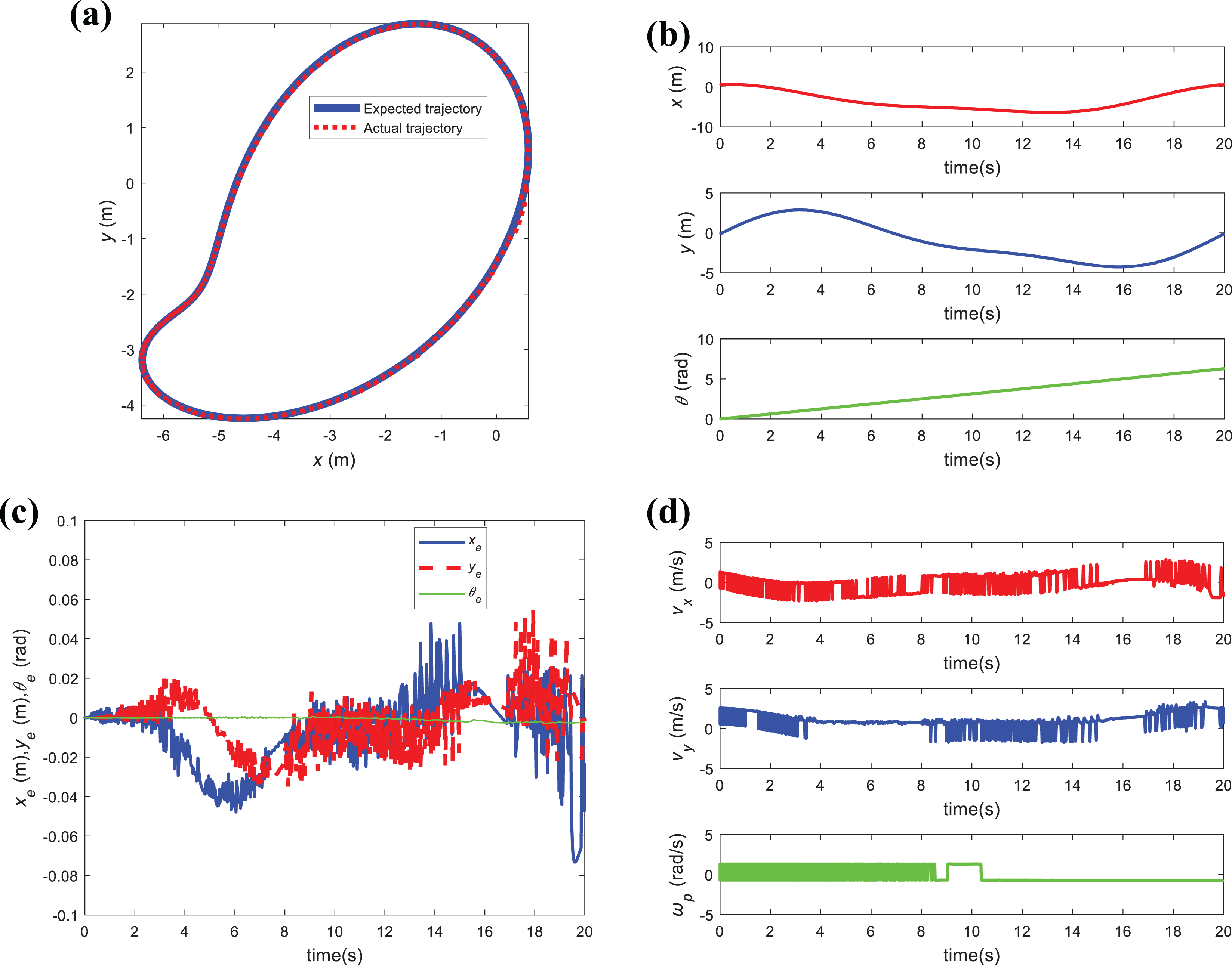
We conducted the simulation experiment of robot tracking irregular trajectory based on the sliding mode controller. We let the initial pose of the mobile robot in the world coordinate system be $x (0) = 0.5$ m, $y (0) = - 0.1$ m, and $θ (0) = 0$ rad. The controller parameters are set as $k_{1} = k_{2} = k_{3} = 20,$ $δ_{1} = δ_{2} = δ_{3} = 1$ . The results of the robot tracking the irregular trajectory are shown in Figure 16. As the robot in Figures 12 to 15 tracks the circular trajectory, the initial position of the robot is inside the circle. Therefore, the tracking error of the robot initially has a large value. However, when the robot tracks the irregular trajectory, the initial position of the robot is on the trajectory. Therefore, the tracking error of the robot is now relatively small initially. It can be seen from Figure 16 that the robot can track irregular trajectory well.

Figure 16.
Simulation curves of tracking irregular trajectory. (a) Irregular trajectory tracking. (b) Curves of the robot pose. (c) Curves of the trajectory tracking error. (d) Curves of the control variables.

The experiment lasted for 20 s. As shown in Figure 16(a), the robot can track the irregular trajectory in a finite time. The responses of the robot pose are shown in Figure 16(b). As shown in Figure 16(c), the error curves had violent tremors according to the irregular trajectory. As shown in Figure 16(d), the control variables $(v_{x}, v_{y}, ω_{p})$ had some tremors.

Simulation of robot positioning control

We assume that the initial pose of the robot is ${[x (k), y (k), θ (k)]}^{T} {=[2,2,0]}^{T}$ . Given the desired velocity, the robot moves in a straight line in the positive direction of the x-axis of the world coordinate system, that is, $v_{b x} = 0.1 m/s, v_{b y} = 0, ω_{b p} = 0$ .

We assume that the standard deviation of the process noise is 0.002, the standard deviation of the observation of the electronic compass is 0.04, the standard deviation of the observation of the ultrasonic sensor is 0.06, and the standard deviation of the observation of the laser scanner is 0.008. The parameters of the mobile robot are set as $α = π /4 rad, r = 0.05 m, L = 0.34 m$ . The sampling period of the robot is $T_{s} = 0.1 s$ . The state curves and error curves of the simulation results are shown in Figures 17 and 18, respectively.

Figure 17.
Curves of the robot. (a) Curves of the state-x. (b) Curves of the state-y. (c) Curves of the state-θ.

Figure 18.
Error curves of the robot. (a) Error curve of the state-x. (b) Error curve of the state-y. (c) Error curve of the state-θ.

The estimate for state x is almost the same as the expected value. In order to show the difference between the two curves, we applied 0.5 ordinate units of translation along the positive direction of Y axis to the green curve, as shown in Figure 17(a). The estimate of state y oscillates around the expected value in Figure 17(b), and its fluctuation range is within the range of $\pm 0.05$ m. The estimate of state θ converges to the expected value in Figure 17(c). As shown in Figure 18, the estimation errors of the three state variables converge to zero. The estimation errors of x and y are within the range of $\pm 0.05$ m, and the estimation of θ converges to zero.

Experiments

Physical prototype

The physical prototype of the robot is shown in Figure 19. The system diagram is shown in Figure 20. Figure 21 and Table 3 show the components of the prototype.

Figure 19.
The physical prototype of the robot. (a) The structure of the physical prototype. (b) Internal structure diagram of the physical prototype. 1. Lidar. 2. Microcontroller. 3. Omnidirectional wheel. 4. Servo motor of the wheel. 5. Gearbox. 6. Servo motor of the X-shaped rotary mechanism. 7. Battery. 8. Absolute encoder. 9. Servo motor of the telescopic mechanism. 10. Gear turntable. 11. Screw.

Figure 20.
Block diagram of the system.

Figure 21.
Physical devices of the system.

Table 3.
Devices used in the robot.

Device name Type Quantity

Controller STM32F407 1

Ultrasonic sensor HC-SR04 6

Infrared sensor E18-D80NK 4

Attitude sensor MPU6050 1

Lidar RPLIDAR A2 1

Bluetooth module ATK-HC05 1

DC brushless motor driver RM-C620 8

Brushless DC motor RM-M3508 P19 8

Motor controller STM32F427 2

Absolute encoder HAE28U5V12A1 4

Proximity switch LJ12A3-4-Z/BX 2

Motion experiments

According to the above kinematics model, we set L and α as constants and set a certain driving angular velocity for each wheel. We can collect data from sensors when the robot moves. We control the servo motor to achieve the angle α of the X-shaped mechanism to the desired angle. Based on the data of the absolute encoders, we can measure the angle α, which is shown in Figure 22. Through the data collected by the absolute encoders, we can know that the two angles $α_{1}$ and $α_{2}$ of the X-shaped mechanism in the final state of the robot are, respectively, −75.41° and −36.035°. α is the average of $α_{1}$ and $α_{2}$ , and is −55.72°.

Figure 22.
Real-time data of the absolute encoders.

Then we let α = 45° and L = 325 mm, the absolute value of the motor angular velocity for each wheel is given as 3500 r/min, and the reduction ratio of the motor is 19:1. According to the kinematics model formula and the above conditions, the trajectory of the robot should be a straight line, and the vehicle’s velocity can be obtained.

Figure 23 shows a group of screenshots from the experiment, in which the robot is moving in a straight line.

Figure 23.
The robot moving in a straight line.

While the robot moves in a straight line, we can get the position of the robot with the data obtained by the laser radar.

The radar data of the robot moving along a straight line are shown in Figure 24. The angle between the obstacle that is in front of the mobile robot and the positive direction of the radar is within 49–53°. From that, we can get the distance information of the robot. Based on the distance and time spent by the robot, we can obtain the average speed of the robot. The distance is 2 m. The robot covered the distance in 1.47 s. Therefore, the average speed is about 1.3605 m/s. According to the angular velocity we set for each wheel of the robot, we can calculate that the velocity of the robot is 1.3640 m/s based on the kinematics equation. It can be found that the theoretical calculation results are consistent with the experiment data.

Figure 24.
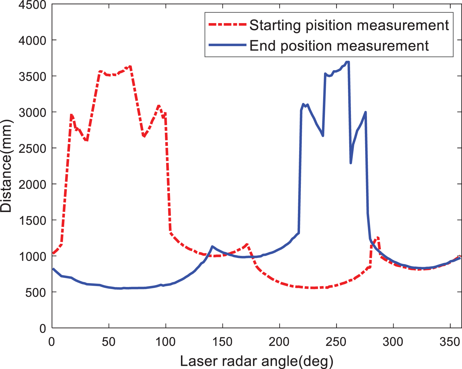
Lidar data for start and end states.

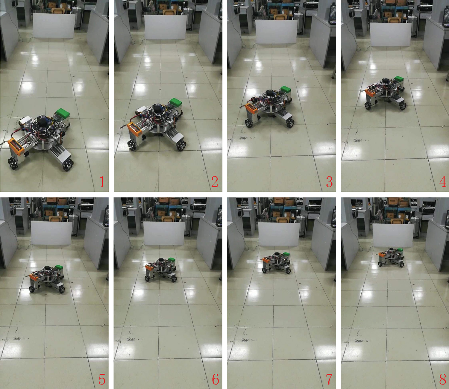
We conducted the experiment of the robot in a narrow environment. Although the robot can pass through a narrow environment, there is a minimum threshold of width. When the width of the narrow environment is larger than this threshold, the robot can pass through it smoothly; otherwise, it cannot pass. The threshold value is determined by the structure size of the robot. When the robot encounters a narrow environment that it is unable to pass due to its wide chassis, it will first detect whether the width is lower than the threshold that it can pass. If the width is higher than the threshold that the robot can pass through, the robot will change its shape and pass through the environment. Figure 25 shows a group of screenshots from the robot passing through the narrow environment.

Figure 25.
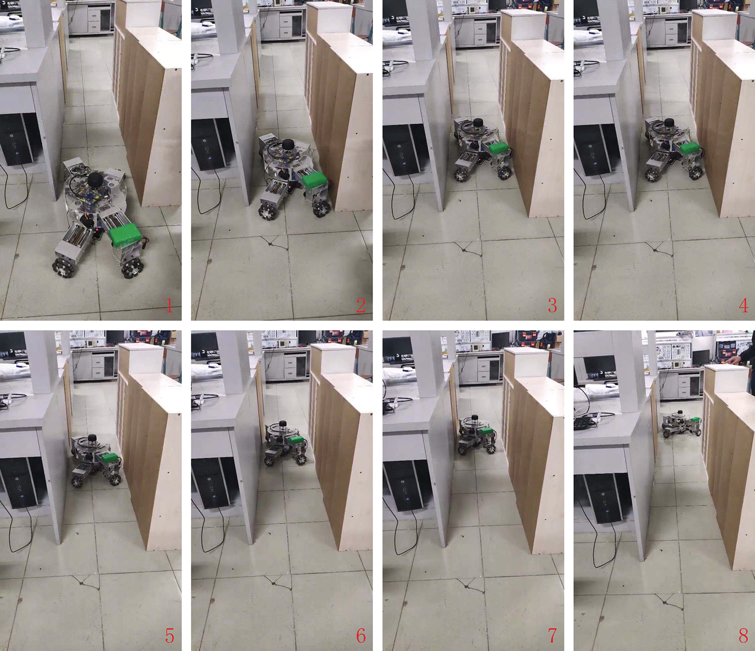
The robot passing through the narrow environment.

We have carried out the experiment of robot deformation. The transformable chassis of the robot can be divided into a telescopic mechanism and an X-shaped mechanism, moving mechanism. The telescopic mechanism is controlled with two motors to realize its translational telescopic motion respectively. Each motor controls two lead screws fixed on one line of the X-shaped mechanism to move synchronously. The X-shaped mechanism is driven by two motors to realize its rotational motion corporately. The angle of the X-shaped mechanism is controlled by those two motors. In other words, the angle between the two lines that constitute the X-shaped structure is $2 α$ .

A group of screenshots of the robot deformation experiment is shown in Figure 26. The robot extends the two lines of X first, then changes the angle between the two lines, and finally returns to the original state. It can be determined that the robot can realize the expansion and contractile motion of telescopic mechanism along the linear guide and that the angle of the X-shaped mechanism can be adjusted effectively. Figure 27 shows the data of the robot deformation experiment as well as the variation of the angles. The four angles are measured by four absolute angular encoders, respectively. Angles 1 and 2 are the rotation angles of the motors that drive the linear guides. Angles 3 and 4 are the rotation angles of the two motors that adjust the angle of the X-shaped mechanism.

Figure 26.
The states of the variable structure mode.

Figure 27.
Data of the absolute encoders.

Conclusion

A wheeled robot with a transformable chassis is proposed in this article. A kinematics model is established according to its motion characteristics and several special motion forms of the robot are analyzed. A trajectory tracking controller is designed based on sliding mode control. An extended Kalman filter algorithm is used to improve the positioning accuracy. The effectiveness of the work is verified by computer simulation. A real prototype of the robot is built. The robot is expected to find broad application in the indoor warehouse environments with flat floors.

$ω_{1}$	$ω_{2}$	$ω_{3}$	$ω_{4}$
360 °/s	−360 °/s	−360 °/s	360 °/s

$ω_{1}$	$ω_{2}$	$ω_{3}$	$ω_{4}$
−360 °/s	360 °/s	−360 °/s	360 °/s

Device name	Type	Quantity
Controller	STM32F407	1
Ultrasonic sensor	HC-SR04	6
Infrared sensor	E18-D80NK	4
Attitude sensor	MPU6050	1
Lidar	RPLIDAR A2	1
Bluetooth module	ATK-HC05	1
DC brushless motor driver	RM-C620	8
Brushless DC motor	RM-M3508 P19	8
Motor controller	STM32F427	2
Absolute encoder	HAE28U5V12A1	4
Proximity switch	LJ12A3-4-Z/BX	2

Footnotes

Declaration of conflicting interests

The author(s) declared no potential conflicts of interest with respect to the research, authorship, and/or publication of this article.

Funding

The author(s) disclosed receipt of the following financial support for the research, authorship, and/or publication of this article: This work was supported by the Natural Science Foundation of China (61105103).

ORCID iD

Lei Guo

Liang Zhao

References

Galasso

Lodi Rizzini

Oleari

, et al. Efficient calibration of four wheel industrial AGVS. Robot Comput Int Manuf 2019; 57: 116–128.

Lin

, et al. A master-slave separate parallel intelligent mobile robot used for autonomous pallet transportation. Appl Sci 2019; 9(3): 368.

Ren

Yang

, et al. Extended state observer-based sliding mode control of an omnidirectional mobile robot with friction compensation. IEEE Trans Indust Elect 2019; 66(12): 9480–9489.

Tun

Huang

Mohan

, et al. Four-wheel steering and driving mechanism for a reconfigurable floor cleaning robot. Automat Construct 2019; 2019: 106.

Boubezoula

Hassam

Boutalbi

. Robust-flatness controller design for a differentially driven wheeled mobile robot. Int J Control Autom Syst 2018; 16(4): 1895–1904.

Shang

Qiu

Yang

, et al. Structure design and performance analysis for locomotion system of the field exploration robot. WSEAS Trans Syst 2011; 10(10): 331–341.

Alipour

Robat

Tarvirdizadeh

. Dynamics modeling and sliding mode control of tractor-trailer wheeled mobile robots subject to wheels slip. Mechanism Mach Theory 2019; 138: 16–37.

Sun

Xiang

, et al. A transformable wheel-legged mobile robot: design, analysis and experiment. Robot Autonom Syst 2017; 98: 30–41.

Rout

Agrawal

Choudhury

. Modeling and control of a six-wheeled mobile robot. In: Proceedings of third international conference on ICTCS 2017, Udaipur, India, 16–17 December 2017, pp. 323–331. Singapore: Springer Nature Singapore Pte Ltd.

10.

Luo

Shang

Wei

, et al. A reconfigurable hybrid wheel- track mobile robot based on watt ii six-bar linkage. Mechanism Mach Theory 2018; 128: 16–32.

11.

Tadakuma

Maruyama

, et al. Armadillo-inspired wheel-leg retractable module. In: 2009 IEEE international conference on robotics and biomimetics (ROBIO), Guilin, Guangxi, China1, 19–13 December 2009, pp. 610–615.

12.

Peng

Wang

Shen

, et al. Cooperative attitude control for a wheel-legged robot. Peer Peer Netwk Appl 2019; 12(6): 1741–1752.

13.

Schwarz

Rodehutskors

Droeschel

, et al. Nimbro rescue: solving disaster-response tasks with the mobile manipulation robot Momaro. J Field Robot 2017; 34(2): 400–425.

14.

Schwarz

Beul

Droeschel

, et al. DRC team Nimbro rescue: Perception and control for centaur-like mobile manipulation robot Momaro. In: Spenko

Buerger

Iagnemma

(eds) The DARPA robotics challenge finals: Humanoid robots to the rescue. Springer tracts in advanced robotics. Vol 121. Cham: Springer, 2018, pp. 145–190.

15.

Panahandeh

Alipour

Tarvirdizadeh

, et al. A kinematic Lyapunov-based controller to posture stabilization of wheeled mobile robots. Mech Syst Signal Proc 2019; 134: 106319.

16.

Jin

Zou

, et al. Backstepping trajectory tracking based on fuzzy sliding mode control for differential mobile robots. J Intel Robot Syst 2019; 96(1): 109–121.

17.

Juman

Wong

Rajkumar

, et al. An incremental unsupervised learning based trajectory controller for a 4 wheeled skid steer mobile robot. Eng Appl Artif Intel 2019; 85: 385–392.

18.

Guo

Pan

. Composite learning robot control with friction compensation: a neural network-based approach. IEEE Trans Indust Elect 2019; 66(10): 7841–7851.

19.

Montoya-Villegas

Moreno-Valenzuela

Perez-Alcocer

. A feedback linearization-based motion controller for a UWMR with experimental evaluations. Robotica 2019; 37(6): 1073–1089.

20.

Korayem

Yousefzadeh

Susany

. Dynamic modeling and feedback linearization control of wheeled mobile cable-driven parallel robot considering cable sag. Arabian J Sci Eng 2017; 42(11): 4779–4788.

21.

Korayem

Yousefzadeh

Manteghi

. Dynamics and input–output feedback linearization control of a wheeled mobile cable-driven parallel robot. Mult Syst Dynam 2017; 40(1): 55–73.

22.

Yazdkhasti

Sasiadek

. Multi sensor fusion based on adaptive kalman filtering. In: Dołęga

Głębocki

Kordos

Żugaj

(eds) Advances in aerospace guidance, navigation and control. Cham: Springer, 2018, pp. 317–333.

23.

Fang

Dai

, et al. A new multisensor fusion slam approach for mobile robots. J Control Theory Appl 2009; 7(4): 389–394.

24.

Ruan

Liu

Ren

, et al. Accurate 2D localization for mobile robot by multi-sensor fusion. In: Proceedings of 2018 IEEE 4th information technology and mechatronics engineering conference, ITOEC, Chongqing, China, 14–16 December 2018, pp. 839–843. New York: IEEE.

25.

Morales

Martínez

, et al. Pure-pursuit reactive path tracking for nonholonomic mobile robots with a 2D laser scanner. EURASIP J Adv Signal Proc 2009; 2009: 1–10.

26.

Harik

EIHC

Korsaeth

. The heading weight function: a novel LiDAR-based local planner for nonholonomic mobile robots. Sensors 2019; 19(16): 3606.

Design and control of a variable structure robot

Abstract

Keywords

Introduction

Structure design

Kinematics analysis

Coordinate system establishment

Kinematics formula

Special forms of movement

Controller design

Trajectory tracking controller design

Mathematical model of trajectory tracking

Sliding mode controller design

Positioning controller design

Establishment and analysis of discrete models

Correction process of the extended Kalman filter

Discussion

Remark 1

Remark 2

Remark 3

Computer simulation

Simulation of kinematics model

In situ rotation

Movement in the x direction

Simulation of trajectory tracking control

Simulation of robot positioning control

Experiments

Physical prototype

Motion experiments

Conclusion

Footnotes

Declaration of conflicting interests

Funding

ORCID iD

References