Vehicle pose estimation algorithm for parking automated guided vehicle

Abstract

Parking automated guided vehicle is more and more widely used for efficient automatic parking and one of the tough challenges for parking automated guided vehicle is the problem of vehicle pose estimation. The traditional algorithms rely on the profile information of vehicle body and sensors are required to be mounted at the top of the vehicle. However, the sensors are always mounted at a lower place because the height of a parking automated guided vehicle is always beyond 0.2mm, where we can only get the vehicle wheel information and limited vehicle body information. In this article, a novel method is given based on the symmetry of wheel point clouds collected by 3-D lidar. Firstly, we combine cell-based method with support vector machine classifier to segment ground point clouds. Secondly, wheel point clouds are segmented from obstacle point clouds and their symmetry are corrected by iterative closest point algorithm. Then, we estimate the vehicle pose by the symmetry plane of wheel point clouds. Finally, we compare our method with registration method that combines sample consensus initial alignment algorithm and iterative closest point algorithm. The experiments have been carried out.

Introduction

Parking problem is becoming a major issue in urban development due to the increase in number of vehicles. Many smart parking systems have been developed in recent years, which mainly focus on parking safety ^1,2 and finding parking space. ³ For space-saving parking, stereo garage is one of the solutions. Parking automated guided vehicle (AGV) is a flexible robot that has been used for automatic parking in flat parking lots. Since there is no need to reserve space for opening vehicle doors, entering and exiting parking stall, the parking space is greatly saved. Besides, parking lot accidents are avoided due to automatic parking and multi-robot cooperations will make parking more efficient. ⁴

A typical parking AGV was designed and developed in 2014. ⁵ It is bigger and lower flexibility than most mobile robots. In 2017, two types of pallet parking AGVs with lidar ⁶ and vision navigation ⁷ were developed, respectively. Like most parking AGVs, an extra mechanical platform for transporting vehicle is primarily provided and users is required to park the vehicle on it accurately. Different from these parking AGVs, clamp-on parking AGV does not rely on the extra mechanical platform and is only required to park the vehicle to parking buffer zone, which effectively reduces security risks and improves user experience. So the vehicle pose estimation technology is required to be adopted. More than 10 years ago, many scholars have begun to research this topic in autonomous driving based on lidar data. In general, these methods can be roughly divided into two categories: feature-based ^{8 –11} and measurement model-based. ^{12 –15}

Since most vehicles are in the shape of a box, the partial profiles of them are like the letter L. Thus, L-shape feature can be used to represent them with a simple structure, which is widely used in feature-based methods. Gan et al. ⁸ and Kim et al. ⁹ proposed an efficient algorithm to fit a cluster of 2-D laser scan points with an L-shape and got the vehicle pose by this feature. Wang et al. ¹⁰ determined the interest area of vehicle point clouds based on L-shape feature, and used RANSAC (Random Sample Consensus) algorithm to fit straight line of points in interest region to calculate the orientation of vehicle. Mertz et al. ¹¹ used line fit and corner fit for features extraction of a segment to estimate vehicle pose. However, just as stated in Morris et al., ¹² feature-based methods are sensitive to noises and interferences.

In measurement model-based methods, vehicles are usually represented as some rectangles or cuboids, and sampling or optimization techniques are used to estimate the vehicle pose. Morris et al. ¹² proposed four-rectangles measurement model to represent vehicle point clouds and used gradient-based optimization method to obtain vehicle pose. Chen et al. ¹³ combined a likelihood-field-based model with scaling series algorithm to realize real-time vehicle pose estimation based on four-rectangles model. Three-rectangles measurement model is proposed by Petrovskaya et al. ¹⁴ and they used importance sampling technique to estimate vehicle pose. Wojke and Häselich ¹⁵ extended Petrovskaya’s method in unstructured environments and realized vehicle pose estimation and tracking in real time. However, the results obtained by measurement model-based methods may be locally optimal because of the inappropriate initial value.

Figure 1 shows a novel clamp-on parking AGV that was introduced in 2018, which is a heavy load smart mobile robot and its maximum load can reach 3 tons but the height of the parking AGV is only 0.125 m. It works by moving to the bottom of the target vehicle and sensors are required to be mounted at a lower height, which greatly limits sensors’ view. Besides, in order to save parking space, the distance between target vehicle and parking AGV is not large. Thus, when we use lidar to collect data, the number of lidar beams hitting on vehicle body would be small and the profile information of the whole vehicle body cannot be obtained. Since feature-based methods and measurement model-based methods rely on the profile information of vehicle body, they cannot be applied in this case.

Figure 1.

Clamp-on parking AGV. AGV: automated guided vehicle.

In 3-D point clouds processing, ground segmentation is very important, which is the precondition of other higher processes, such as obstacle detection, object classification, and recognition. Generally, approached of ground segmentation include cell-based methods ^{16 –19} and model-based methods. ^{20 –22}

Cell-based method was firstly proposed by Thrun et al. ¹⁶ They project 3-D point clouds to 2.5-D grids and segment the ground point clouds by calculating the maximum height difference of each cell, which was widely used in the 2007 DARPA Grand Challenge competition. ¹⁷ Because Thrun’s method relies on the minimum and maximum height of the points in the cell, it cannot segment the overhanging structures. Thus, Douillard et al. ¹⁸ proposed an improved cell-based method based on cell’s gradient. If the gradient is less than the given threshold, the cell is the ground cell. Based on gradient threshold, Vu et al. ¹⁹ combined adaptive break point detection with mean height evaluation to segment the ground point clouds. The algorithm obtains a better result in uneven and sparse regions than Douillard’s method. Because the cell-based methods only use the local information, they are sensitive to observation noises.

Model-based methods segment the ground by fitting geometric shape of point clouds. Himmelsbach et al. ²⁰ proposed a method for segmenting large-scale remote 3-D point clouds. The method divides the polar grid map into many segments and uses the line extraction algorithm to estimate local ground plane. Different from Himmelsbach’s method, Chen et al. ²¹ used Gaussian process regression to classify ground and obstacles for each segment in polar grid map. Because the point clouds are divided into independent segments, the continuity of the overall ground height cannot be guaranteed. Since the ground is flat in most cases, Lam et al. ²² used the plane RANSAC algorithm followed by the least square fitting on point cloud data to segment the ground point clouds. However, it will over-segment ground point clouds because the surface of some obstacles may be parallel to the ground.

In this article, we propose a vehicle pose estimation method based on the symmetry of wheel point clouds for the clamp-on parking AGV, which can be used to estimate vehicle pose when the mounting heights of sensors are very low. Before wheel point clouds segmentation, we combine Thrun’s cell-based method with support vector machine (SVM) classifier ²³ to segment ground point clouds. The global information and local features of point clouds are used. It has a good performance and is not sensitive to the observation noises.

The rest of this article is structured as follows. In the next section, we introduce the ground segmentation algorithm based on cell-based method and SVM classifier. The third section elaborates the steps of the vehicle pose estimation algorithm with 3-D lidar. The experiments and results are offered in the fourth section. Finally, we summarize this article in the fifth section.

Research on ground segmentation algorithm

Figure 2 is the procedures of ground segmentation. Firstly, we use cell-based method and pass-through filter to pre-segment some ground point clouds and obstacle point clouds, respectively. Then, the normal vectors and height features from pre-segmented point clouds are extracted. Next, these features will be trained as the training data of SVM classifier. Finally, we use the optimal model of SVM classifier to predict the ground and obstacle point clouds.

Figure 2.

Procedures of ground segmentation.

Ground and obstacle pre-segmentation

We take a W × W plane in xy plane and divide it into N × N cells, as shown in Figure 3. The point clouds are projected vertically to the cell plane. Thus, for a point p (x, y, z) in lidar coordinate system, the cell it belongs to is

$p\in C\left[x\cdot \frac{N}{W}+\frac{N}{2}\right]\left[y\cdot \frac{N}{W}+\frac{N}{2}\right]$

1

where W × W is the plane size and N × N is the number of cells. The first cell is the lower-right cell. The threshold is set to h and the maximum height difference △h of each cell is calculated. If △h ≥ h, the cell is set to a ground cell. All points in ground cell form the ground point clouds. The input point clouds and the ground pre-segmentation results are shown in Figure 4(a) and (b), respectively.

Figure 3.

Cell-based method.

Because the height of obstacle point clouds is higher than ground point clouds, a lower threshold of pass-through filter in z-axis direction that is larger than the average height of the ground point clouds segmented by cell-based method is given and the upper threshold is 2 m. Besides, the points far from the lidar center are filtered. Thus, we can get a part of obstacle point clouds, as shown in Figure 4(c).

Figure 4.

Point clouds pre-segmentation. (a) Input point clouds, (b) ground pre-segmentation by cell-based method, and (c) obstacles pre-segmentation by pass-through filter.

Ground and obstacle classification based on SVM classifier

Since the driving area is relatively flat, the normal vectors of ground point clouds will be approximately parallel to the z-axis of lidar coordinate system. Besides, the height of the ground is lower than the obstacles. Therefore, the normal vectors and the height of the points are extracted as the SVM training features.

For a point, its normal vector coincides with the normal of the tangent plane of the surface formed by this point and its neighbors. Thus, it can be obtained by principal component analysis method. ²⁴ Let the k-nearest points set of a point p is P = {p ₁, p ₂,…, p_k } and we can get the corresponding covariance matrix C as follows

$C=\frac{1}{k}{\left[\begin{array}{c}{p}_1-\overline{p}\\ \dots \\ p_k-\overline{p}\end{array}\right]}^T\left[\begin{array}{c}{p}_1-\overline{p}\\ \dots \\ p_k-\overline{p}\end{array}\right]$

2

where $\overline{P}$ is the center of gravity of P. Let λ ₁, λ ₂, and λ ₃ be the eigenvalues of the covariance matrix C, 0 ≤ λ ₁ ≤ λ ₂ ≤ λ ₃, and the eigenvectors corresponding to the eigenvalues are n ₁, n ₂, and n ₃

$C\cdot n_j={\lambda }_j\cdot n_j,j\in \left\{1,2,3\right\}$

3

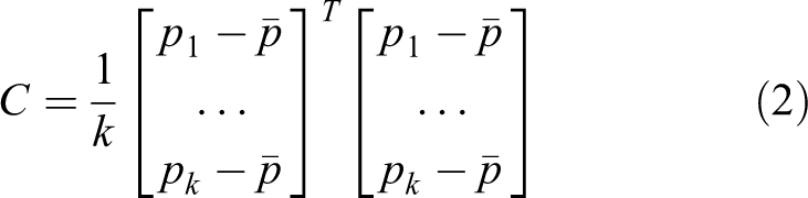
where n ₁ (n_x , n_y , n_z ) is the normal vector of p. The normal estimation result of point clouds is shown in Figure 5. Therefore, the feature vector of the point is n (n_x , n_y , n_z , h), where h is the height of the point.

Figure 5.

Normal estimation of point clouds.

After feature extraction, we can get the training data x

$x=\left[\begin{array}{cc}\begin{array}{cc}{n}_{x_1}& n_{y_1}\\ n_{x_2}& n_{y_2}\end{array}& \begin{array}{cc}{n}_{z_1}& h_1\\ n_{z_2}& h_2\end{array}\\ \begin{array}{cc}\dots & \dots \\ n_{x_N}& n_{y_N}\end{array}& \begin{array}{cc}\dots & \dots \\ n_{z_N}& h_N\end{array}\end{array}\right]$

4

where N is the number of pre-segmented point clouds. The ground point clouds are set to the positive samples and the obstacles point clouds are set to the negative samples. Thus, the training model is

$f\left(W\right)=\text{sign}\left(W^{T}x+b\right)$

5

The optimization function is

$\text{max margin}\left(W,b\right)=\text{max}\underset{W,b,x_i}{\text{min}}\frac{1}{\Vert W\Vert }\left|W^T{x}_i+b\right|$

6

After getting the optimal solution of W and b, we can use the model to predict whether a point is a ground point or an obstacle point. In order to avoid under-segmentation, the points below the average height of ground point clouds will eventually be filtered.

Vehicle pose estimation based on 3-D lidar

Wheel point clouds segmentation

Since the lidar is mounted at a very low height, when parking AGV is behind the vehicle, the vehicle point clouds collected by the lidar mainly consist of two parts: wheel point clouds and chassis point clouds. As shown in Figure 6, the shape of the vehicle point clouds is like the letter n and the wheel point clouds are segmented from obstacle point clouds based on this feature.

Figure 6.

Vehicle feature. (a) n-shape feature of vehicle and (b) n-shape feature of vehicle point clouds.

The minimum height of each cell can be calculated based on cell-based method. The vehicle cell is set to the suspended obstacle cell if the minimum height is greater than the given threshold. Because the distance between parking AGV and target vehicle is small, vehicle chassis point clouds contain more points than other suspended objects. We use Euclidean cluster algorithm ²⁵ to cluster the point clouds of suspended objects and select the largest cluster as the vehicle chassis point clouds. In Euclidean cluster algorithm, if the distance between two points is small, they belong to the same cluster.

As shown in Figure 7, the wheel point clouds is under the vehicle chassis point clouds. Thus, a sector region of interest based on vehicle chassis point clouds can be defined to segment wheel point clouds. The Gaussian distribution of horizontal azimuth ζ for each points is marked as follows

$\zeta \sim N\left(\mu , {\sigma }^2\right)$

7

Figure 7.

Vehicle chassis point clouds.

The angular range of sector region of interest is defined as [μ − 2σ, μ + 2σ] and the radius r of the sector is 4 m, as shown in Figure 8.

Figure 8.

Sector region of interest.

The points outside the sector region will be filtered. Then, the Euclidean cluster algorithm is used to cluster the nonsuspended point clouds and the two clusters with the largest number of points are the wheel clusters.

Correction of wheel symmetry

In theory, left and right wheels are strictly symmetrical. However, because the distances from lidar center to left and right wheels are always different, when using lidar to collect point cloud data, the number of points in left and right wheel point clouds will probably be different, which causes the symmetry errors of the wheel point clouds. Thus, it is necessary to correct the wheel point clouds before obtaining its symmetry plane. In this article, the symmetry of the wheel point clouds is corrected by registration algorithm.

To improve the registration accuracy, number of the left and right wheel point clouds should be balanced. The vertical angle ω of each point p(x, y, z) can be calculated as follows

$\omega =a\text{tan}\left(\frac{z}{\sqrt{x^2+y^2}}\right)$

8

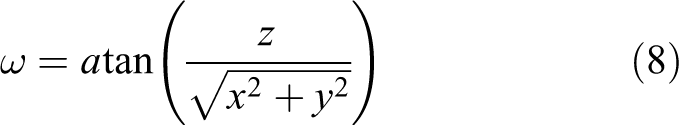
The points are classified into the same category with the same vertical angle. If the proportion that the number of points belong to the same wheel point clouds is small, the category will be filtered.

Assuming that the residual wheel point clouds C is {p ₁, p ₂,…, p_n } and p_i is a point, the center of gravity of the point clouds C is given by

$W_g=\frac{1}{n}\sum _{i=1}^n{p}_i=\frac{1}{2}\left(L_g+R_g\right)$

9

where L_g (x_lg , y_lg , z_lg ) and R_g (x_rg , y_rg , z_rg ) are the center of gravity of the left and right wheel point clouds, respectively.

Let W_g be (x_wg , y_wg , z_wg ) and we can get the normal vector of the symmetry plane

$n_p=\left(A,B,C\right)=\left(x_{rg}-x_{lg},y_{rg}-y_{lg},z_{rg}-z_{lg}\right)$

10

Therefore, the symmetry plane equation is

$Ax+By+Cz-\left(A{x}_{wg}+B{y}_{wg}+C{z}_{wg}\right)=0$

11

The symmetry point $p_i^{\prime }$ of p_i (x_i , y_i , z_i ) with respect to the symmetry plane is

$\left[\begin{array}{c}{x}_i^{\text{′}}\\ y_i^{\text{′}}\\ z_i^{\text{′}}\end{array}\right]=-\left(\frac{A{x}_i+B{y}_i+C{z}_i+D}{A^2+B^2+C^2}\right)\cdot \left[\begin{array}{c}A\\ B\\ C\end{array}\right]+\left[\begin{array}{c}{x}_i\\ y_i\\ z_i\end{array}\right]$

12

where D is $A{x}_{wg}+B{y}_{wg}+C{z}_{wg}$ .

The symmetry point is calculated for each point in left wheel point clouds and we can get the symmetry point clouds L′ of the left wheel point clouds L. Let the right wheel point clouds S be [p ₁, p ₂,…, p_n ] and the symmetry point clouds L′ be $[p_1^{\prime },p_2^{\prime },\dots ,p_m^{\prime }]$ .

We assume the Euclidean Transformation T from L′ to S is (R, t). The iterative closest point (ICP) algorithm minimizes the distances between points in S and L′. ²⁶ In each iteration, ICP computes the correspondences between S and L′, and then (R, t) is calculated to minimize the objective function

$\underset{R,t}{\text{min}}J=\sum _{i=1}^n\sum _{j=1}^m{\omega }_{i,j}{\Vert p_i-\left(R{p}_i^{\text{'}}+t\right)\Vert }^2$

13

where ω_i,j is the weight of correspondence. The maximum matching threshold d _max of point pairs is given before registration. If the distance between a point pair is greater than d _max, ω_i,j = 0. Otherwise, ω_i,j = 1. After ICP registration, we can get the aligned point clouds. The aligned point clouds and the left wheel point clouds form the new wheel point clouds.

Vehicle pose estimation based on wheel symmetry

The homogeneous coordinates of a point in 3-D space can be represented as p = [x y z 1] ^T . After ICP registration, we can get the new wheel point clouds H ₁

$H_1=\left[\begin{array}{cc}L& T\cdot L^{\prime }\end{array}\right] =\left[\begin{array}{cc}\begin{array}{ccc}{x}_1& \dots & \begin{array}{cc}{x}_m& \dots \end{array}\\ y_1& \dots & \begin{array}{cc}{y}_m& \dots \end{array}\\ z_1& \dots & \begin{array}{cc}{z}_m& \dots \end{array}\end{array}& \begin{array}{c}{x}_{m+n}\\ y_{m+n}\\ z_{m+n}\end{array}\\ \begin{array}{ccc} 1& \dots & \begin{array}{cc}1& \dots \end{array}\end{array}& 1\end{array}\right]$

14

Thus, the normal vector of symmetry plane P ₁ of point clouds H ₁ is n ₁ = [a ₁ b ₁ c ₁] ^T , where c ₁ > 0. The angle α between P ₁ and xy plane is

$\alpha =-\frac{b_1}{\Vert b_1\Vert }\cdot {\text{cos}}^{-1}\left(\frac{c_1}{\sqrt{a_1{}^2+b_1{}^2+c_1{}^2}}\right)$

15

In order to reduce the influence of unevenness on the ground, we rotate the wheel point clouds H ₁ α around the x-axis and we can get

$H_2=\left[\begin{array}{cc}\begin{array}{cc}1& 0\\ 0& \text{cos}\hspace{0.17em}\alpha \end{array}& \begin{array}{cc}0& 0\\ -\text{sin}\hspace{0.17em}\alpha & 0\end{array}\\ \begin{array}{cc}0& \text{sin}\hspace{0.17em}\alpha \\ 0& 0\end{array}& \begin{array}{cc}\text{cos}\hspace{0.17em}\alpha & 0\\ 0& 1\end{array}\end{array}\right]\cdot H_1$

16

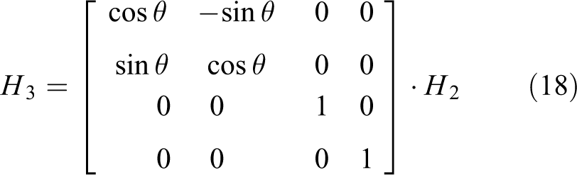
The symmetry plane P ₂ of point clouds H ₂ is perpendicular to xy plane. Assuming that the normal vector of P ₂ is n ₂ = [a ₂ b ₂ c ₂] ^T , where b ₂ > 0, the horizontal azimuth of the target vehicle with respect to the lidar is given by

$\text{θ}=-\frac{a_2}{\Vert a_2\Vert }\cdot {\text{cos}}^{-1}\left(\frac{b_2}{\sqrt{a_2{}^2+b_2{}^2+c_2{}^2}}\right)$

17

We rotate the wheel point clouds H ₂ θ around the z-axis of the lidar coordinate system and we can get the new wheel point clouds H ₃ is

$H_3=\left[\begin{array}{cc}\begin{array}{cc}\text{cos}\hspace{0.17em}\theta & -\text{sin}\hspace{0.17em}\theta \\ \text{sin}\hspace{0.17em}\theta & \text{cos}\hspace{0.17em}\theta \end{array}& \begin{array}{cc}0& 0\\ 0& 0\end{array}\\ \begin{array}{cc}0& 0\\ 0& 0\end{array}& \begin{array}{cc}1& 0\\ 0& 1\end{array}\end{array}\right]\cdot H_2$

18

The symmetry plane of H ₃ is parallel to xz plane. Thus, the distance in y-direction between vehicle center and lidar center is

$\text{Δ}y=\frac{1}{m+n}\left(\text{sin}\hspace{0.17em}\theta \sum _{i=1}^{m+n}{x}_i+\text{cos}\hspace{0.17em}\alpha \hspace{0.17em}\text{cos}\hspace{0.17em}\theta \sum _{i=1}^{m+n}{y}_i-\text{sin}\hspace{0.17em}\alpha \hspace{0.17em}\text{cos}\hspace{0.17em}\theta \sum _{i=1}^{m+n}{z}_i\right)$

19

We translate H ₃ to Δy and we can get the final wheel point clouds. In theory, the symmetry plane of final wheel point clouds is coincident with xz plane. We suppose the xz plane of lidar coordinate system is coincident with the bilateral symmetry plane of parking AGV. Thus, in order to align to the target vehicle, the adjustment of parking AGV is

$P={\left[\begin{array}{cc}-\text{Δ}y& -\theta \end{array}\right]}^T$

20

where Δy is the traverse displacement and θ is the rotation angle.

Registration method combing SAC-IA and ICP algorithms

If we have the source point clouds at the origin location, the object pose can be obtained by registration method. ²⁷ In ICP algorithm, the maximum matching threshold d _max should be given to get the correspondent points. If the distance between two point clouds is large, d _max should also be large. However, large matching threshold will cause incorrect correspondences, which will make registration failed. Thus, initial transformation should be calculated by rough registration if there is no overlap between two point clouds.

Point feature histograms (PFH) is a 3-D feature descriptor, which represents the surface model properties of a point. Fast point feature histograms (FPFH) is a simplified form of PFH and its computation is more time-saving than PFH. ²⁸ We assume the neighbors of point p is N = {p ₁,…, p_n }, where points in N are in the sphere. Sphere’s radius is r and p is the center. For each pair of points p and p_k in N, we calculate their normal vectors n and n_k . The angular variation of n and n_k is

$\left[\begin{array}{c}\alpha \\ \beta \\ \theta \end{array}\right]=\left[\begin{array}{c}v\cdot n_k\\ \left(u\cdot \left(p_k-p\right)\right)/\Vert p_k-p\Vert \\ {\text{tan}}^{-1}\left(w\cdot n_k,u\cdot n_k\right)\end{array}\right]$

21

where u = n, v = (p − p_k ) × u, w = u × v. The angular variations of each point pair consist of the simplified point feature histograms (SPFH). Thus, the FPFH of point p is

$\text{FPFH}\left(p\right)=\text{SPFH}\left(p\right)+\frac{1}{k}\sum _{i=1}^k\frac{1}{{\omega }_k}\cdot \text{SPFH}\left(p_k\right)$

22

where k is the k neighbors of point p and ω_k is the distance between point p and point p_k .

After getting the FPFH features of the whole point clouds, we use sample consensus initial alignment (SAC-IA) algorithm ²⁸ to register the point clouds. Different from ICP algorithm, SAC-IA algorithm finds the correspondence of a point by FPFH features and the rigid transformation $T_i^{\prime }$ for each point pair will be calculated. The performance of $T_i^{\prime }$ is evaluated by

$J=\sum _{i=1}^{n}H\left(e_i\right)$

23

where H(e_i ) is a Huber penalty measure

$H\left(e_i\right)=\left\{\begin{array}{c}0.5e_i{}^2\\ 0.5t_e\left(2\Vert e_i\Vert -t_e\right)\end{array}\begin{array}{c}\Vert e_i\Vert \le t_e\\ \Vert e_i\Vert >t_e\end{array}\right.$

24

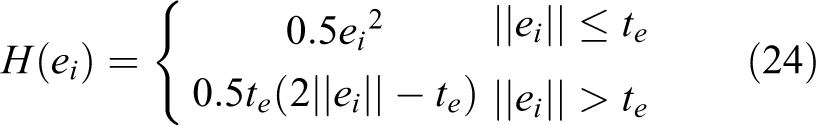
where t_e is a given threshold and e_i is the distance between the target point clouds and the aligned point clouds transformed by the transformation of the ith matching point pair. Finally, we find the best transformation from all transformations to minimize J.

After SAC-IA registration, we can get the initial transformation T ₁ and the aligned point clouds $H_1^{\prime }$ . Then, we use ICP algorithm to register point clouds $H_1^{\prime }$ to the target point clouds and we can get the transformation T ₂. Thus, the transformation T′ from original point clouds to target point clouds is T ₂ T _1. If the target point clouds are the wheel point clouds whose symmetry plane is coincident with the xz plane of lidar coordinate system, the adjustment of parking AGV is

$P^{\prime }={\left[\begin{array}{cc}-\text{Δ}{y}^{\prime }& -{\theta }^{\text{'}}\end{array}\right]}^T={\left[\begin{array}{cc}-{\text{sin}}^{-1}\left(T^{\prime }\left[0\right]\left[1\right]\right)& T^{\prime }\left[1\right]\left[3\right]\end{array}\right]}^T$

25

Experiments and results

The lidar used in this article is Velodyne VLP-16 and the experimental platform is shown in Figure 9. In order to get the vehicle point clouds from the obstacle point clouds, the ground point clouds should be segmented first. Figure 10 shows the ground segmentation results. It can be seen that the ground point clouds below the vehicle are erroneously segmented to obstacles by cell-based method but there are almost no ground point clouds in obstacle point clouds by our method. Our method can get a better result.

Figure 9.

Experimental platform.

Figure 10.

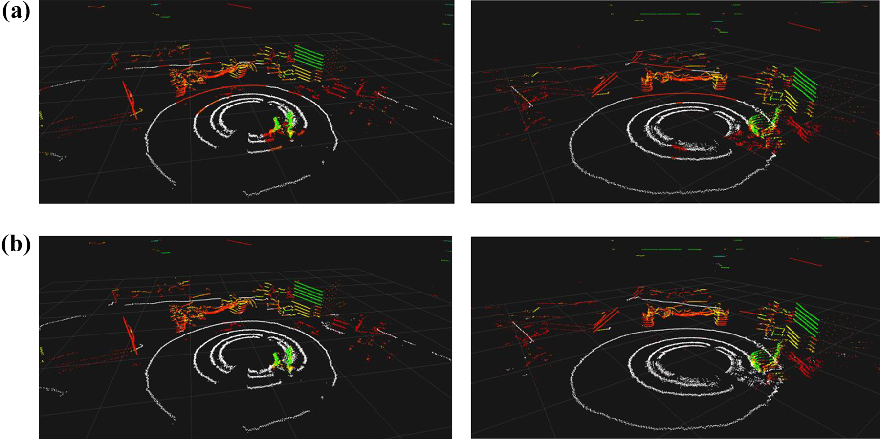
Results of ground segmentation. (a) Results of ground segmentation by cell-based method and (b) results of ground segmentation by our method.

Figure 11 is the results of vehicle segmentation. The vehicle chassis point clouds can be segmented effectively by suspended object extraction and Euclidean cluster algorithm, as shown in Figure 11(a). After that, the wheel point clouds are extracted as the nonsuspended objects from the sector region of interest, as shown in Figure 11(b).

Figure 11.

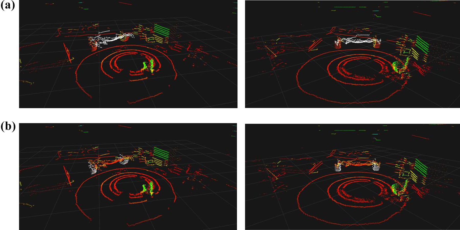
Results of vehicle segmentation. (a) Results of vehicle chassis segmentation and (b) results of vehicle wheel segmentation.

Because the point clouds of the left and right wheels are not strictly symmetrical, the symmetry of the wheel point clouds should be corrected. Figure 12 shows the correction results. In Figure 12(a), white point clouds are the symmetry point clouds of the left wheel with respect to the symmetry plane of the wheel point clouds. We can find that the symmetry point clouds are not coincident with the right wheel point clouds and there are symmetry errors in wheel point clouds. After registration, the coincidence degrees of the wheel point clouds increase and the symmetry errors decrease, as shown in Figure 12(b).

Figure 12.

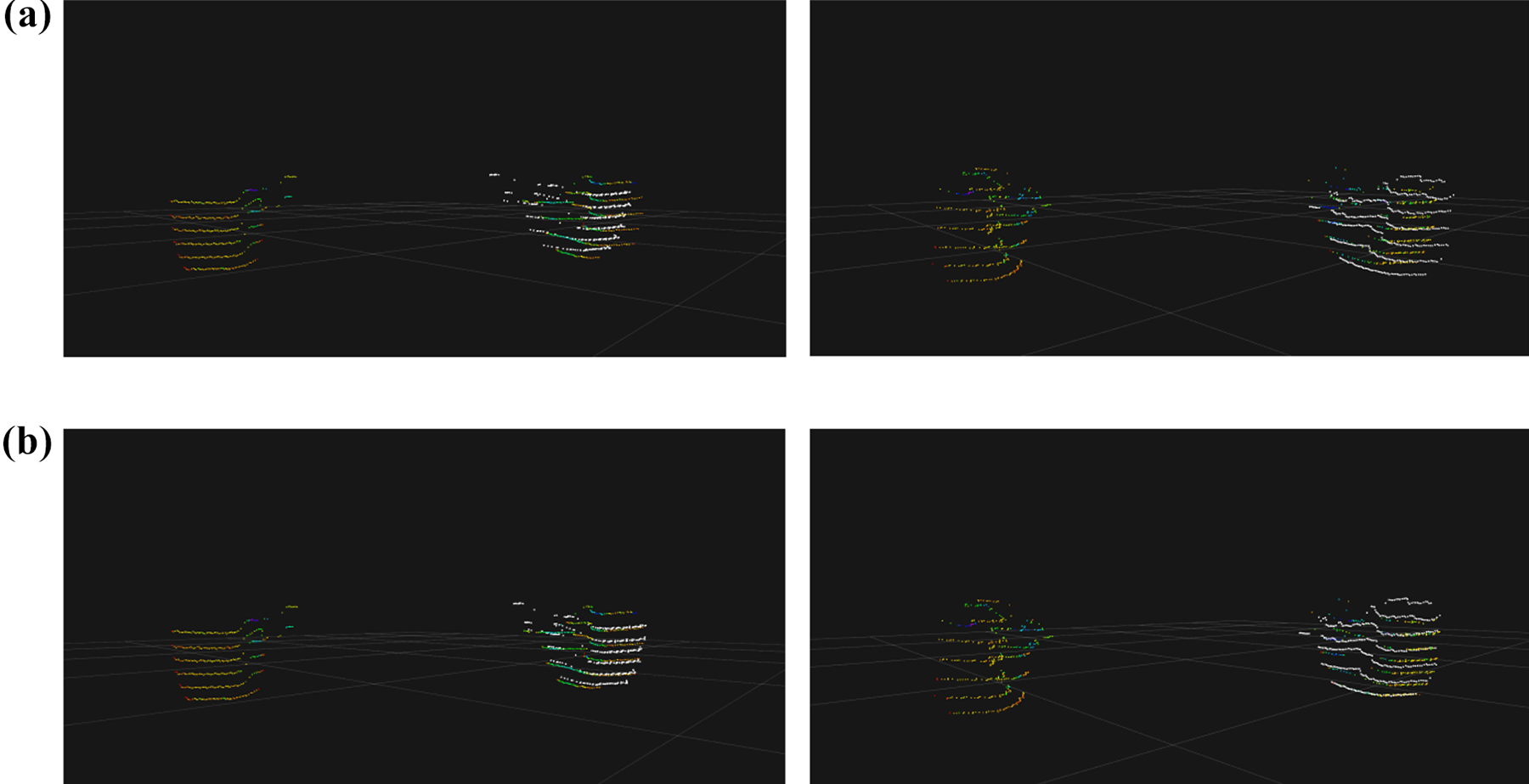
Correction results of wheel symmetry. (a) Wheel point clouds before registration and (b) wheel point clouds after registration.

To get the vehicle pose, the corrected wheel point clouds are transformed. Figure 13 shows the transformed results of wheel point clouds (white point clouds) by the vehicle pose estimation algorithm. It can be seen that the symmetry planes (white plane) of wheel point clouds are coincident with the xz plane. In this case, lidar on parking AGV has aligned to the target vehicle. For comparison, we combine SAC-IA algorithm with ICP algorithm to register the wheel point clouds. The target point clouds are the wheel point clouds sampled by the lidar when the xz plane is coincident with the symmetry plane of the vehicle. The original point clouds are the current wheel point clouds segmented by our algorithm. As shown in Figure 14, the original point clouds are coincident with the target point clouds after registration.

Figure 13.

Vehicle pose estimation by transforming wheel point clouds.

Figure 14.

Vehicle pose estimation by registration method combining SAC-IA algorithm with ICP algorithm. SAC-IA: sample consensus initial alignment; ICP: iterative closest point.

In order to evaluate the precision of the vehicle pose estimation algorithm proposed in this article, we rotated and moved the lidar to different places. The lidar data were recorded by robot operating system (ROS) and we took out 100 scans from it to calculate the vehicle pose respectively. Figure 15 is the estimation results of horizontal azimuth and Figure 16 is the estimation results of distance in y-direction. It can be seen that the results of our method are basically coincident with the registration method. Figure 17 is the Euclidean fitness scores of registration method, which are the sum of squared distances from aligned point clouds to target point clouds. The lower Euclidean fitness scores mean the better registration results and the vehicle pose estimation results are more accurate. From Figure 17, we can find that the Euclidean fitness scores are very low. Thus, the registration precision is high.

Figure 15.

Estimation results of horizontal azimuth.

Figure 16.

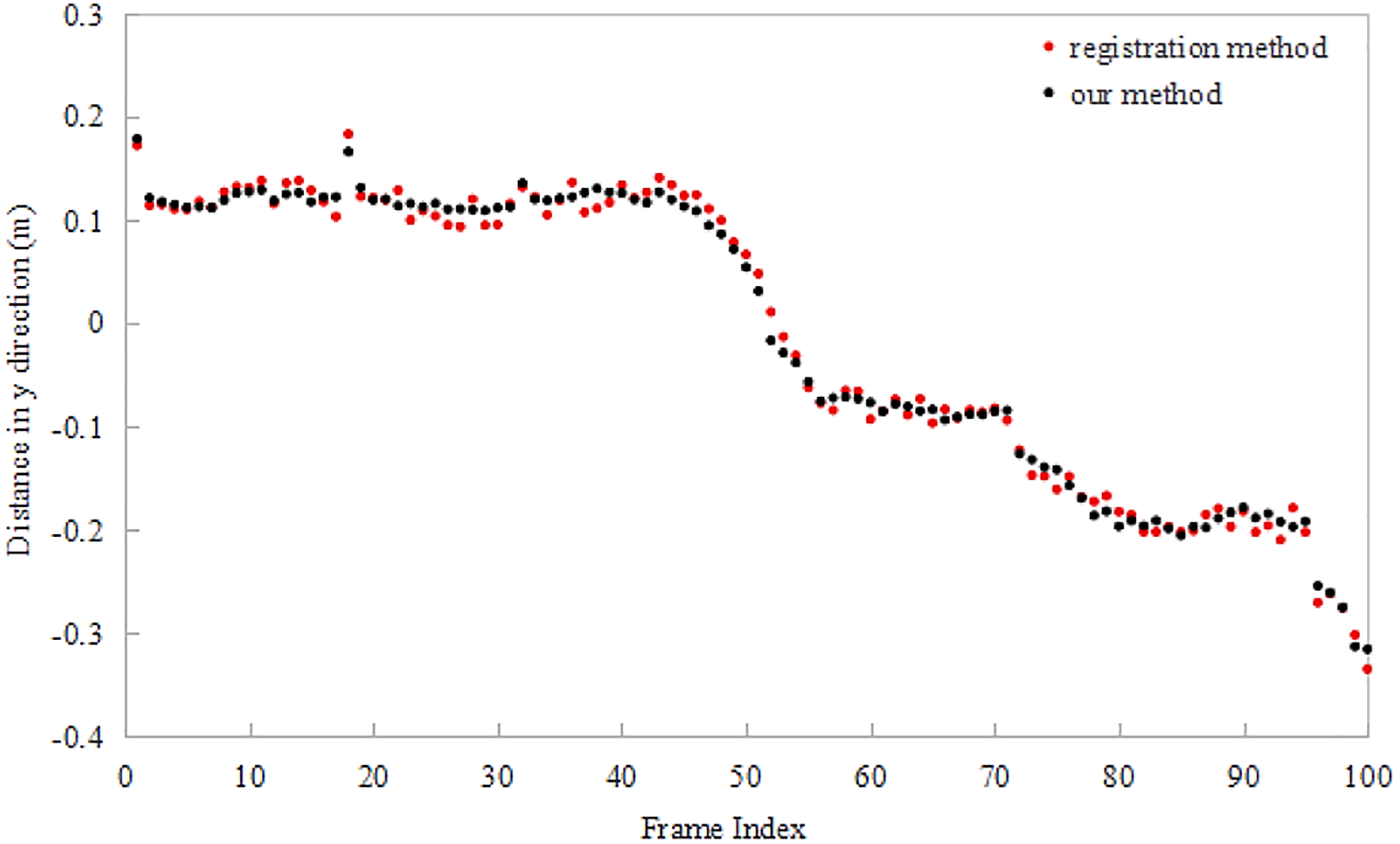
Estimation results of distance in y-direction.

Figure 17.

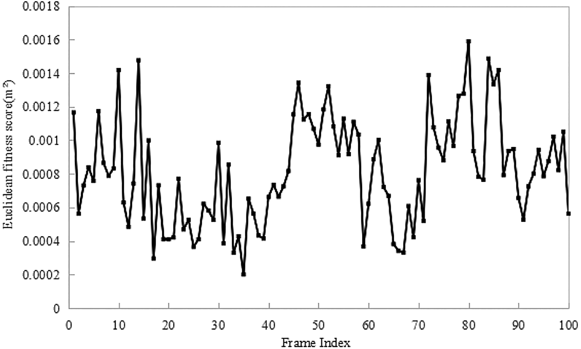
Euclidean fitness score of registration method.

The processor used in this article is a standard laptop (Intel Core-i5-3749 CPU 3.2GHZ, 8G RAM) and the algorithm is run in ROS environment (C++). Figure 18 shows the processing time of vehicle pose estimation algorithm. It can be seen that the processing speed of our method is faster than registration method. The processing time consumption of our method is mainly in SVM classifier training and ICP registration.

Figure 18.

Processing time of vehicle pose estimation algorithm.

Conclusions

By combining cell-based method with SVM classifier, the preparation procedure of training data is simplified and the results of ground segmentation are more exactly. The method by extracting the symmetry plane of the wheel point clouds solves the vehicle pose estimation problem in the case where the vehicle body information cannot be obtained. The registration method is given to provide a reference of vehicle pose because the registration accuracy is high according to the Euclidean fitness scores. The vehicle pose estimation results of our method are basically coincident with registration method and more time-saving. Besides, our method can estimate the pose of different vehicle models but registration method needs to build a database of different wheel point clouds models to provide the target registration point clouds. Experimental results indicate that the vehicle pose estimation method in this article is feasible and it has a high precision, which can be used on parking AGV.

In the future, we will consider data fusion of vision and lidar. Vehicle wheels recognition and regions of interest determination are implemented by vision, and then the vehicle pose is estimated based on lidar data. Besides, real-time performance of the algorithm should be improved for providing real-time feedback to the robot, which would probably improve the robustness and precision of the algorithm.