Sage Journals: Discover world-class research

Abstract

The article deals with design issues of a system for regulating and controlling of the pendulum amplitude using an inertial system and a stepper motor. Basis of the solution is the pendulum theory and its mathematical model, respectively mathematical modeling of the pendulum trajectory. The aim is to derive the mathematical equation of the pendulum, calculate its oscillation period, and plot the oscillation of the pendulum model with damping or actuating in real time on a case study, as proposed by the authors. Following is the description of the inertial system, which is represented by an accelerometer and an angle sensor. Information about the velocity, acceleration, and position of the pendulum are acquired by mathematical derivations. The proposed hardware model and amplitude control algorithm for the microcontroller together with a brief description of the concluded experiments, which were focused on the accuracy of measurement and evaluation of all acquired data, is described next. The obtained results can be applied in the field of robotics, mainly due to its accuracy of trajectory calculation and plotting but also by reverse validation control of the movement of the monitored robot effectors.

Keywords

Sensors actuator power drive pendulum microcontroller robot

Introduction

In industrial and automation control systems, control or evaluation circuits, consisting of a sensor and a measuring member, are often used. Such a connection is called a measurement chain, which serves either for measurement purposes or is also involved in feedback control or regulation. The measured variables in this case are motion variables such as path, acceleration rate, or direction of motion. Evaluation of such parameters requires application of a motion model with known motion ratios.

Robotics and automation have a significant supporting role in the manufacturing industry nowadays, sensors are an inseparable part of this role, due to their ability to obtain control data for robotic and automation systems. Many problems occur during sensors application, for example, measurement, calibration, data collection, data processing, filtering data errors, and so on. The article is therefore focused on dealing with issues of regulation and control system of a pendulum mass of bob oscillation in laboratory conditions.

A good example for the application of the proposed model could be the self-balancing mobile robotic system—the Segway. In recent years, the two-wheeler has been widely used for its benefits such as energy saving, environmental protection, simple structure, flexible operation, and so on. Research in the field of robotics has great potential, theoretical significance, and practical application. In 1986, Yamato Gaoqiao, Professor of Tokyo Electric Communication University, designed a dual coaxial and stand-alone mobile robot at first. In 2002, the first two-wheeled self-balancing vehicle, the Segway human transporter, was produced, by which the design of a micro-electro-mechanical systems (MEMS)-based two-wheeled self-supporting electric vehicle was improved. On the other hand, many researchers^1–8 have focused their analysis on the stability and design of a control system of two-wheeled self-balancing robots. In the area of control, Ravichandran and Mahindrakar presented a design of a controller and used a strategy that combined Lyapunov’s redesign and time scaling. They verified the methodology by using it in a two-wheeled robot, thus applying robust stabilization for the area of insufficient mechanical systems by using the time scaling. The Lyapunov’s controller for self-balancing two-wheeled vehicles has examined the design and validation of the controller for the inertial two-wheeled vehicle using the Lyapunov feedback control technique, which is applied and implemented in this article, which addresses the more precise control of the pendulum oscillation in such way, that the initial, set oscillation was still maintained by a control variable and did not fall below a predetermined value. The predetermined value is with minimal tolerances, ensuring a more enjoyable use of the self-balancing mobile robotic system—the Segway.

Theoretical and practical basics

Inertial system

The basis of an inertial system is the first and second Newton’s law of motion (equation (1))

a = \frac{F}{m} (m \cdot s^{- 2})

where a is a vector of acceleration, F is a vector of power, and m weight of the body.

Inertial sensors include gyroscopes and accelerometers, which are required to calculate the direction and movement of a body in space in an own inertial coordinate system. Navigation based on an inertial system is completely independent of external devices, but a disadvantage in the form of error incrementation in time still exists.

Each free object in space has six degrees of freedom, therefore an inertial navigation system (INS) consists of three gyroscopes and three accelerometers (one gyroscope and one accelerometer for each axis x, y, z).^9

–12

INS implemented on a pendulum in robotics

The application of INS in robotics aims to measure the relative movement in a robotic system, where the position of the robotic arm (speed and orientation in the robot workstation), with a known initial position, should continuously be determined.¹³

The magnitude and direction of acceleration action and angular speed of the robot effector in relation to the initial value is determined, followed by a double integration by time to acquire precise information of the relative robot movement in accordance to its programmed trajectory. Integration of parameters impacts the measurement error and creates a deviation of the calculated position from the actual one.¹⁴ Even with utilization of sensors with very high error correction, the measurement error cannot be eliminated.

Case study

Mathematical model

Pendulum

The pendulum is characteristic by the oscillating motion around its equilibrium position.¹⁵ The repetitive conversion of positional energy to kinetic and vice versa is applied when the pendulum moves. The physical parameters of the pendulum include the moment of inertia, determined by the mass and geometric shape of the pendulum, the torque moment, determined as a product of a distance from the pivot (swing radius) and the force that is perpendicular to the pendulum arm.^16,17 The angular oscillation, velocity, and acceleration of the pendulum are considered vital for the purposes of this article.

The greatest potential energy of a pendulum bob can be achieved in the most extreme position of pendulum oscillation and the smallest in its most vertical position (equilibrium position), on the other hand the greatest kinetic energy of a pendulum bob can be achieved during the transition through its vertical position and the smallest in its most extreme position of oscillation.^11,18

By ignoring the friction forces and resistance of the environment, a pendulum should oscillate without lowering its amplitude of oscillation.¹⁹ Under 5° oscillation, the pendulum swings in relation to time in a sinus movement, the oscillation period is determined by the length of the hinge and the size of the gravity acceleration (equation (2))

T = 2 π \sqrt{\frac{l}{g}}

Above 5° oscillation, the oscillation period is exponentially dependent on the amplitude size (see Figure 1).

Figure 1.

Dependence of the oscillation period on the amplitude size.

Equation of motion

For the purpose of this article, a case study dealing with control of pendulum oscillation aimed to preserve the initial swing angle by implementation of a stepper motor with an attached cart to deliver the required control variable change was chosen. Figure 2 illustrates the pendulum with an attached cart used in this case study.

Figure 2.

Pendulum with an attached cart.

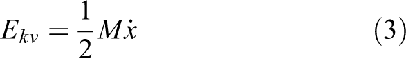
Kinetic energy of the cart E_kv can be calculated as follows (equation (3))

E_{k v} = \frac{1}{2} M \dot{x}

Calculation of the kinetic power of the pendulum requires the expression of the pendulum position by x_k and y_k coordinates (a shift caused by the position of the cart occurs for the x_k ) (equation (4))

k = l s i n φ + x y_{k} = l c o s φ

Derivation with respect to time yields (equation (5))

v_{k x} = l c o s \dot{φ} c o s φ + \dot{x} v_{k y} = - l s i n \dot{φ} s i n φ

The square root for pendulum speed v_k can be defined as (equation (6))

| \vec{v_{k}} |^{2} = v_{k x}^{2} + v_{k y}^{2} = l^{2} \dot{φ} + \dot{x} + l \dot{y} \dot{x} c o s φ

which translates to (equation (7))

E_{k k} = \frac{1}{2} m l^{2} {\dot{φ}}^{2} + \frac{1}{2} m \dot{x} + m l \dot{φ} \dot{x} c o s φ

The total kinetic energy of the system is defined as (equation (8))

E_{k} = E_{k k} + E_{k v} = \frac{1}{2} (M + m) {\dot{x}}^{2} + \frac{1}{2} m l^{2} {\dot{φ}}^{2} + m \dot{φ} \dot{x} c o s φ

Kinetic energy calculated from individual acceleration speeds cannot be determined in a similar fashion. The nonlinear character of pendulum and cart movements causes the Lagrange equation of the second type to not be independent. The variable $m l \dot{φ} \dot{x} c o s φ$ needs to be determined. Potential energy of the cart is constant, its equation for the pendulum is defined as (equation (9))

E_{p k} = - m g l c o s φ

The equation for the Lagrange function for the designed system (equation (10))

L = E_{k} - E_{p}

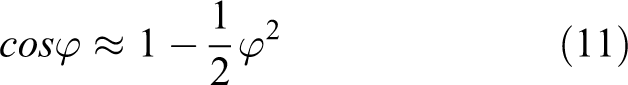
Taylor series (equation (11)) is utilized to address small deflections and speeds of oscillation by modifying the Lagrange function for potential energy of pendulum (equation (12))

c o s φ \approx 1 - \frac{1}{2} φ^{2}

\bar{L} = \frac{1}{2} (M + m) {\dot{x}}^{2} + \frac{1}{2} m l^{2} {\dot{φ}}^{2} + m l φ \dot{x} - \frac{1}{2} m g l φ^{2}

Lagrange equation of the second type (equation (13))

\frac{d}{d t (\frac{\partial L}{\partial \dot{q_{j}}})} - (\frac{\partial L}{\partial q_{j}}) = 0

for j = 1, 2…n, where q_j is the jth general coordinate and L is a Lagrange function.

After implementation of the aforementioned formulas, approximations and derivations, the equation for linear harmonic oscillator with angular frequency ω (equation (14)). Generalization produces the coordinate φ (equation (15))

ω = \sqrt{\frac{M + m}{M}} \sqrt{\frac{g}{l}}

φ = A c o s (\sqrt{\frac{M + m}{M}} \sqrt{\frac{g}{l}} t + φ 0)

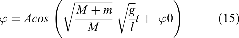
The aforementioned formula determines the period of swing of the pendulum bob, which can be used to determine the time period of the cart motion. The formula was altered for the purpose of these calculations (equation (16)), derived and used in equation (17) to produce equation (18)

φ = A c o s (ω t + φ 0)

\ddot{χ} = - \frac{m}{M + m} l \ddot{φ}

χ = ω^{2} \frac{m}{M + m} l A c o s (ω t + φ 0)

Substitution of ω and derivation generates (equation (19))

x = - \frac{m}{M + m} l A c o s (\sqrt{\frac{M + m}{M}} \sqrt{\frac{g}{l}} t + φ 0) v_{0 t} + x_{0}

where v ₀ and are the integration constants and represent the initial speed and the initial position with respect to the coordinate x. The negative value of the first member of the equation addresses the opposite direction of the cart movement in relation to the pendulum. Solving the given function produced the equations for cart and pendulum position (equations (19) and (20))

φ = A c o s (\sqrt{\frac{M + m}{M}} \sqrt{\frac{g}{l}} t + φ 0)

Hardware model

For the purpose of this case study, a physical pendulum was chosen as a model, a rotary movement sensor was mechanically fixed to the pivot point of the pendulum to collect data. Determination of the direction of rotation was achieved by an incremental motion sensor.

A block diagram of the hardware system used in this case study can be seen in the Figure 3, it consists from these modules: Accelerometer (AM), Operational Amplifier (OA), Microcontroller (MC), Bridge Driver (BD), Stepper Motor (SM), USB to UART Converter (C), and Personal Computer (PC).

Figure 3.

Block diagram of module interconnection.

Accelerometer

An accelerometer is a compact device designed to measure nongravitational acceleration. The accelerometer proposed in this design is based on the MEMS technology, it is an integrated circuit consisting of three-axis analog accelerometer with an excellent heat stability. The accelerometer is capable of static gravity acceleration, dynamic acceleration, impact and vibration measurements by utilizing microscopic crystals, which go under stress during vibrations and therefore generate voltage to create a reading on any acceleration.^20,21

Its input range is ±3 g and for an input voltage of 3.6 V is equal to an output voltage of 360 mV/g. The user defines the width of the transmission band with three capacitors C_x, C_y, C_z , connected to the individual outputs of the accelerometer X _out , Y _out , Z _out. These capacitors must be connected if a LOWPASS filter for antialiasing and noise reduction is being utilized. The implementation of accelerometer and the direction of gravitation effect toward the accelerometer is shown in the Figures 4 and 5, respectively.

Figure 4.

Gyroscope an accelerometer implementation into INS. INS: inertial navigation system.

Figure 5.

Gravitation effect toward axes of an accelerometer.

Microcontroller

Processing of the analogue signal in the microcontroller requires its conversion into a digital form. The proposed microcontroller already contains an A/D converter to deal with the conversion along with an UART interface (used for sending data to a computer) and several digital input–output interfaces to control the stepper motor to modify the pendulum amplitude.

The process of analogue signal sampling was utilized by applying the Nyquist–Shannon theorem, which defines the minimum sampling frequency f_vz by considering the x(t) signal to be twice as high as the highest frequency f_x _max, which is included in the signal. Equation (21) is used to calculate of the output digital value for the A/D converter

A D C = \frac{V_{in} × 2^{n}}{V_{ref}}

where V _in is the input voltage, V _ref is the reference voltage, and n represents the converter resolution.

Situation of ±1 g gravitational force was considered. In this situation, the x-axis was only gravitationally accelerated by +1 g, the output voltage changed to 1.93 V (1.57 V + 0.36 V) in this direction and to 1.21 V (1.57 V − 0.36 V) in the opposite one (−1 g). The subtraction of these voltages is 0.72 V (1.93 V − 1.21 V).

The A/D converter utilizes a 10-bit resolution, but the input signal transmits only 8-bit values, therefore a division by 4 is required for the input values. The analogue signal needs to be modified to reflect a state, where gravitational force +1 g is equal to a voltage of 5 V, −1 g is equal to a voltage of 0 V, and 0 g is equal to a voltage of 2.5 V.

The proposed modification of input signal allows the microcontroller to perform conversion into its digital form, where the total number of 256 bits is halved. The first 128 bits correspond to a movement caused by the +1 g gravitational force, the second 128 bits correspond to movement in the opposite direction (−1 g gravitational force), which is reflected in ADC _min/max value (equation (22))

A D C = \frac{1024}{4} = 256 bit

To optimize processing speed, sampling was performed every 15 ms, therefore the total number of samples during 1 s was 66 (1/0.015). The period of pendulum oscillation was 0.88 s, which produced 58 samples for each pendulum oscillation, which translates to 29 samples for each (positive and negative) direction of pendulum oscillation.

USB to UART converter

Since the incremental sensor cannot be directly connected to a personal computer, an integrated circuit was used, to process sensor signals by utilizing an application developed specifically for this purpose. The microcomputer is also connected to the communication input–output units such as digital display or serial data interface for PC communication.

The analogue voltage from an accelerometer is enhanced and modified by the operational amplifier to allow for measurement by the microcontroller. The voltage is then converted into a digital form using the A/D converter of the microcontroller and at the same time sent to the computer using a USB to UART converter.

The converter converts and sends serial data from UART microcontroller interface by a USB connection to a PC. The received data are processed and used to plot the movement of the accelerometer utilizing an application developed for this purpose. Parallelly, digital data are processed by a microcontroller and the error value is evaluated, subsequently the movement of the stepper motor is driven by a full bridge driver to deliver the control variable change.

Software model

Base position

The first step for the software realization of this case study was to move the cart of the pendulum to its designated base position. The position in question is located approximately in the center of linear shift trajectory of the cart.

The algorithm utilizes a photoelectric sensor located on the left side of the shift trajectory of the pendulum cart, which represents its left most extreme position. The stepper motor moves the cart to the left, until the desired extreme position is reached by the cart (the cart must be blocking the beam of the photoelectric sensor). Upon reaching this destination, the cart is automatically moved in the opposite direction until it reaches its base position (the number of steps for the stepper motor to reach this position is known in advance).

Automatic oscillation

The next stage for the algorithm was the initial swing of pendulum, which was done by programming an automatic initial oscillation. The first condition states, that a stepper motor will run four steps to move the cart, if no interruption of a steady light beam has been recorded by a photoelectric sensor. After 300 ms, another four steps in the opposite direction will be performed. This cycle is repeated four times in a row.

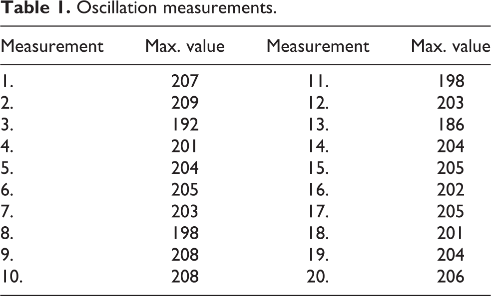
The number of the steps of a stepper motor determines the size of the initial amplitude of the pendulum. To compare, the similarity of the initial oscillation, 20 experiments (Table 1) were performed, each one was measured from the equilibrium position of the pendulum.

Table 1.

Oscillation measurements.

Measurement	Max. value	Measurement	Max. value
1.	207	11.	198
2.	209	12.	203
3.	192	13.	186
4.	201	14.	204
5.	204	15.	205
6.	205	16.	202
7.	203	17.	205
8.	198	18.	201
9.	208	19.	204
10.	208	20.	206

Detection of position

Detection of the position is used to direct the movement of the cart (based on the value of a bit named direction) to increase the amplitude. The opposite movement of the cart (in relation to the pendulum) would decrease the amplitude. The tracking deviates from the initial oscillation of the pendulum (immediately after the automatic oscillation).

The utilization of the y-axis for measurement has an advantage in a steady and strong signal but also a disadvantage in the form of a double signal period and a minimum signal value for both extreme positions, so the exact position of the pendulum could not be exactly determined.

To cope with this issue, a function for position detection was implemented, where the algorithm initially detects the transition of pendulum bob through the equilibrium position and the direction in which it moves to change the bit direction accordingly. The value of direction will its value to 1 if it is moving to the left or 0 if it is moving to the right. The main loop of the algorithm changes the value of the bit direction between 1 (if the movement of the pendulum bob is to the left) and 0 (if the movement of the pendulum bob is to the right) only if the pendulum bob is passing through the equilibrium position.

Maximum value

The largest and smallest value measured from the accelerometer (the largest and lowest amplitude) are recorded by the algorithm after the automatic oscillation takes place. One hundred measurements were performed to determine the largest and smallest one, these two are stored in two variables and serve only for a comparison with the currently measured values. The largest stored value is used as a reference for evaluation of the error value.

Another function has been programmed to record the current maximum measured value to reflect the decrease/increase of the amplitude. Subsequently, the function compares the current maximum measured value with the highest referenced one. If the currently measured maximum value is less than a reference maximum value reduced by 11 (value determined during the testing phase of the hardware model), an error variable is generated with a value equal to the difference calculated. The stepper motor will react to the error value and behave as a control variable moving the pendulum to a side according to the value of the direction bit. The diagram of the software model algorithm is depicted in Figure 6.

Figure 6.

Diagram of the software model algorithm.

Graphical application

The pendulum oscillation is displayed in a graphical application developed in Visual Studio 2013. The application receives data from a serial port of the microcontroller to plot the movement of the pendulum. An example of plotting the movement of pendulum bob in the developed application with indicated its left and right extreme positions and transition of equilibrium position is shown in Figure 7.

Figure 7.

Example of the movement of pendulum bob.

Experiments concluded

After the development of the mathematical, hardware and software aspect of the model, various experiments were concluded to study the movement characteristics of the proposed model. Figure 8 shows the first movement of the pendulum from its stable position until the end of automatic oscillation. This procedure lasted approximately 10 s. The signal is disturbed only at the bottom of the amplitude, which represents the extreme positions of pendulum movement. The distortion is caused by the stepper motor that has started to move in the opposite direction before reaching the extreme position.

Figure 8.

Pendulum movement until the end of automatic oscillation.

The impact of control variable change on the pendulum movement (Figure 9) was another characteristic to study. The sinus movement characteristic of pendulum was disrupted by the movement of the stepper motor, which occurs if the value of the control variable changes.

Figure 9.

Detail of control variable change impact on pendulum movement.

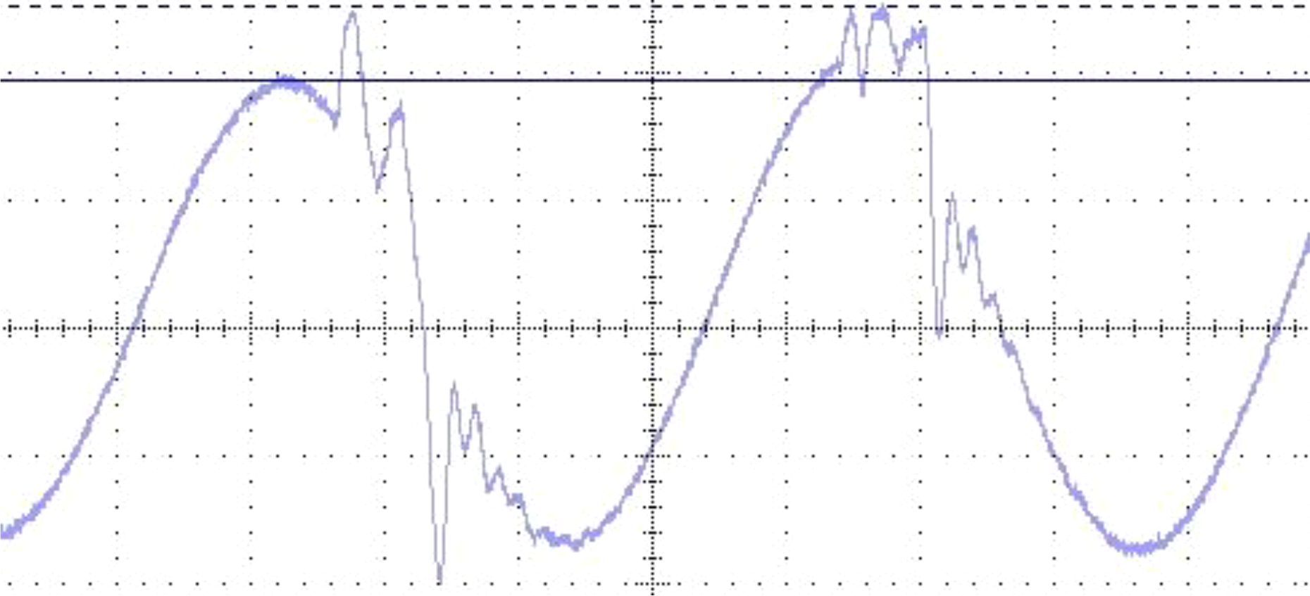
Figure 10 shows the movement characteristic of pendulum before (left half of the raster) and after a change in value of a control variable took place (right half of the raster). The amplitude of the voltage before the change was 3.50 V, after the change has occurred, the value has risen to 3.68 V. If the desired angle value of oscillation setpoint was 35° for the 3.68 V, then one degree of oscillation has a value of 0.105 V (3.68/35).

Figure 10.

Movement characteristic of pendulum before and after a change in value of a control variable.

The oscillation period for two different angles of deflection (35° and 10°) was measured to study if a change in value of a control variable has the same constant effect on the amplitude change (Figures 11 and 12). Twenty measurements were performed, from which an evaluation of the amplitude value change before and after the value of a control variable has changed (shown in Table 2).

Figure 11.

Signal measured for period with 10° oscillation.

Figure 12.

Signal measured for period with 35° oscillation.

Table 2.

Measurements of Δ amplitude value change.

Measurement	Δ Amplitude (mV)	Measurement	Δ Amplitude (mV)
1.	160	11.	80
2.	220	12.	160
3.	160	13.	160
4.	80	14.	80
5.	60	15.	160
6.	200	16.	160
7.	80	17.	160
8.	80	18.	160
9.	140	19.	160
10.	140	20.	160

The concluded experiments show in some cases considerable differences in the measured data. Sometimes the cart moves only once in one of the directions, which corresponds to a small change in the amplitude, but on other occasions moves more than once in both directions, which corresponds to a big change in the amplitude.

This behavior can be greatly influenced by a nonstandard signal generated during the change of value of a control variable, which leads to the stepper motor moving the cart as a reaction to the error value. The cart motion may interfere with the information from the A/D converter, where several measurements with a low measured voltage will take place. The measurements can be evaluated as a reason for another change of the control variable value, which is subsequently realized. Figure 13 shows a detail of such a signal, where the green signal indicates the desired behavior of the signal and the red signal indicates the location of the undesired voltage drop.

Figure 13.

Detail of a nonstandard signal.

Conclusion

In the described research, nonlinear modeling of reduced dynamics, control, and automatic excitation—balancing of the adjusted amplitude of the oscillation was presented. The authors have chosen a case study dealing with control of pendulum oscillation aimed to preserve the initial swing angle by implementation of a stepper motor with an attached cart to deliver the required control variable change. A physical pendulum was chosen with a rotary movement sensor mechanically fixed to the pivot point of the pendulum to collect data. Determination of the direction of rotation was achieved by an incremental motion sensor. Equation of motion of the pendulum bob was derived and calculated together with the oscillation period. Information about the velocity, acceleration, and position of the pendulum were acquired by mathematical derivations. For positioning constraints, limitation was included directly into the motion equations. Obviously, the external force model is suitable for the description of the examined type of pendulum limitation.

The obtained results can be applied in the field of robotics, mainly due to its accuracy of trajectory calculation and plotting but also by reverse validation control of the movement of the monitored robot effectors. The proposed model is applicable for simulating a two-wheeled self-balancing mobile robotic system or other unstable robotic transport means with parallel wheel arrangement from a physics perspective. Robotic devices belonging to this category of robotic systems require a certain degree of intelligence (autonomous behavior), which is called mobile service robots. A convenient addition for the exact regulation and control of mobile service robots is the implementation of an inertial navigation that provides reverse validation and reverse control, for example, for a tilting system of a two-wheeled self-balancing mobile robotic system.

Footnotes

Declaration of conflicting interests

The author(s) declared no potential conflicts of interest with respect to the research, authorship, and/or publication of this article.

Funding

The author(s) disclosed receipt of the following financial support for the research, authorship, and/or publication of this article: The contribution is sponsored by the project 015STU-4/2018. Specialized laboratory supported by multimedia textbook for subject “Production systems design and operation” for STU Bratislava and by the project 013TUKE-4/2019: Modern educational tools and methods for forming creativity and increasing practical skills and habits for graduates of technical university study programs. This publication has been written thanks to support of the Operational Program Research and Innovation for the project: “Výskum pokročilých metód inteligentného spracovania informácií”, ITMS code: NFP313010T570 co-financed by the European Regional Development Found.

References

Nemec

Janota

Gregor

, et al. Control of the mobile robot by hand movement measured by inertial sensors. Electr Eng 2017; 99(4): 1161–1168.

Pirník

Hruboš

Nemec

, et al. Integration of inertial sensor data into control of the mobile platform. Adv Intell Syst 2015; 511: 271–282.

Pivarčiová

Božek

Turygin

, et al. Analysis of control and correction options of mobile robot trajectory by an inertial navigation system. Int J Adv Robot Syst 2008; 15(1): 1–15.

Soták

. Application of wavelet analysis to inertial measurements. Sci Mil J 2008; 2. SPP–852_08-RO02_RU21-240, http://www.novatel.com/assets/Documents/Bulletins/APN064.pdf (accessed 15 April 2017).

Madgwick

. Oscillatory motion tracking with x-IMU, https://github.com/xioTechnologies/Oscillatory-MotionTracking-With-x-IMU (2013, accessed 27 April 2017).

Lim

JLA

Daud

, et al. Development of real-time control system for single-wheeled inverted pendulum platform. In: 2011 IEEE 5th international conference on robotics, automation and mechatronics (RAM), Qingdao, China, September 2011, pp. 131–136. Qingdao: IEEE.

Hehn

D’Andrea

. A flying inverted pendulum. In: 2011 IEEE international conference on robotics and automation, Shanghai, China, May 2011, pp. 763–770. Shanghai: ICRA.

Ionica

Modreanu

Morega

, et al. Design and modeling of a hybrid stepper motor. In: 2017 10th international symposium on advanced topics in electrical engineering (ATEE), Bucharest, Romania, March 2017, pp. 192–195. Romania: ATEE.

Wang

Liang

, et al. Vision-aided inertial navigation for small unmanned aerial vehicles in GPS-denied environments. Int J Adv Robot Syst 2013; 10(6): 276–288.

10.

Qazizada

Pivarčiová

. Mobile robot controlling possibilities of inertial navigation system. Procedia Eng 2016; 149:404–413.

11.

Pivarčiová

Božek

Turygin

, et al. Analysis of control and correction options of mobile robot trajectory by an inertial navigation system. Int J Adv Robot Syst 2018; 15(1): 20–35.

12.

Lobo

Lucas

Dias

, et al. Inertial navigation system for mobile land vehicles. In: Proceedings of the IEEE international symposium on industrial electronics, ISIE’95, Athens, Greece, 10–14 July 1995, pp. 843–848.

13.

Turygin

Božek

Nikitin

, et al. Enhancing the reliability of mobile robots control process via reverse validation. Int J Adv Robot Syst 2016; 13(6): 1–8.

14.

Božek

Pokorný

Svetlík

, et al. The calculations of Jordan curves trajectory of the robot movement. Int J Adv Robot Syst 2016; 13(5): 7.

15.

Qassem

Abuhadrous

Elaydi

. Modeling and simulation of 5 DOF educational robot arm. In: 2nd IEEE international conference on advanced computer control, ICACC, vol. 5, Shenyang, China, March 2010, pp. 569–574.

16.

Rajan

Kumar

Kavitha

. Robust control methods for swing-up and stabilization of a rotary inverted pendulum. In: 2016 international conference on emerging technological trends (ICETT), India, October 2016, pp. 1–6. India: ICETT.

17.

Oltean

. Swing-up and stabilization of the rotational inverted pendulum using PD and fuzzy-PD controllers. Proc Tech 2014; 12: 57–64.

18.

Navin

Koteswara

. Swing up and stabilization control of a rotary inverted pendulum. In: 10th IFAC international symposium on dynamics and control of process systems 2013; 46(32): 654–659.

19.

Kumagai

Ochiai

. Development of a robot balancing on a ball. In: 2008 international conference on control, automation and systems, Seoul, Korea, October 2008, pp. 433–438. Seoul: ICCAS.

20.

Bezák

Božek

Nikitin

Advanced robotic grasping system using deep learning. In: Procedia Engineering: The 6th international conference on modelling of mechanical and mechatronic systems, MMaMS 2014, Vysoké Tatry, Slovakia, 25–27 November 2014, pp. 10–20.

21.

Kim

Jeong

, et al. Kernel ridge regression with lagged-dependent variable: applications to prediction of internal bond strength in a medium density fiberboard process. IEEE T Syst Sci Cyb 2012; 42(6): 1011–1020.

Measurement	Max. value	Measurement	Max. value
1.	207	11.	198
2.	209	12.	203
3.	192	13.	186
4.	201	14.	204
5.	204	15.	205
6.	205	16.	202
7.	203	17.	205
8.	198	18.	201
9.	208	19.	204
10.	208	20.	206

Measurement	Δ Amplitude (mV)	Measurement	Δ Amplitude (mV)
1.	160	11.	80
2.	220	12.	160
3.	160	13.	160
4.	80	14.	80
5.	60	15.	160
6.	200	16.	160
7.	80	17.	160
8.	80	18.	160
9.	140	19.	160
10.	140	20.	160

Measurement	Max. value	Measurement	Max. value
1.	207	11.	198
2.	209	12.	203
3.	192	13.	186
4.	201	14.	204
5.	204	15.	205
6.	205	16.	202
7.	203	17.	205
8.	198	18.	201
9.	208	19.	204
10.	208	20.	206

Measurement	Δ Amplitude (mV)	Measurement	Δ Amplitude (mV)
1.	160	11.	80
2.	220	12.	160
3.	160	13.	160
4.	80	14.	80
5.	60	15.	160
6.	200	16.	160
7.	80	17.	160
8.	80	18.	160
9.	140	19.	160
10.	140	20.	160

Nonlinear modeling of the arm dynamics for the manipulators with reverse sensory validation

Abstract

Keywords

Introduction

Theoretical and practical basics

Inertial system

INS implemented on a pendulum in robotics

Case study

Mathematical model

Pendulum

Equation of motion

Hardware model

Accelerometer

Microcontroller

USB to UART converter

Software model

Base position

Automatic oscillation

Detection of position

Maximum value

Graphical application

Experiments concluded

Conclusion

Footnotes

Declaration of conflicting interests

Funding

References

Measurement	Max. value	Measurement	Max. value
1.	207	11.	198
2.	209	12.	203
3.	192	13.	186
4.	201	14.	204
5.	204	15.	205
6.	205	16.	202
7.	203	17.	205
8.	198	18.	201
9.	208	19.	204
10.	208	20.	206

Measurement	Δ Amplitude (mV)	Measurement	Δ Amplitude (mV)
1.	160	11.	80
2.	220	12.	160
3.	160	13.	160
4.	80	14.	80
5.	60	15.	160
6.	200	16.	160
7.	80	17.	160
8.	80	18.	160
9.	140	19.	160
10.	140	20.	160