
Abstract
This article presents a new control algorithm for the omnidirectional motion of a legged robot on uneven terrain based on an analytical kinematic solution without the use of Jacobians. In order to control the robot easily and efficiently in all situations, a simplified circle-based workspace approximation has been introduced. Foot trajectories for legged robot movement were generated on concentric circular paths around an analytically computed common centre of motion. This systematic motion model, together with new gait control variables that can be changed during legged robot motion, enabled the implementation of a new adaptive gait phase control algorithm, as well as the addition of algorithms for ground-level adaptation, 3-dimensional map-based step adjustment and fusion of all corrections to establish and/or maintain foot contact with the ground. The method being applicable to different legged robot designs was performed and tested on the laboratory prototype of a hexagonal hexapod robot, and the results of the experiments showed the practical value of the proposed adaptive yaw control method (available also as a video supplement).
Introduction
The phenomenon of walking has been the subject of research for decades, focusing on two-legged (birds, kangaroos, humans), four-legged (amphibians, reptiles, mammals), six-legged (insects), eight-legged (spiders, scorpions, crabs) and multi-legged (centipedes) living beings. Compared to walking on flat terrain, walking on uneven terrain brings into play unexpected balance perturbations, loss of footholds, abrupt changes of site view and blockage of legs, which when combined create a handful of new technical challenges. 1 –6
It is known that the periodicity of fixed gaits becomes a drawback on uneven terrain. The way around this is to use free gaits which would enable direction-driven motion. 7 –9 A very specific and most demanding problem is keeping a desired direction of motion on uneven terrain without losing pace and stability. In many cases, the posture of a robot is also significant for fulfilling a given task. 10,11 This leads to a general problem of omnidirectional motion on uneven terrain, that is, efficient yaw control in three dimensions. 12 –14 Numerous researchers have been tackling this problem in different ways. As stated in the study by Wettergreen and Thorpe, 15 control, behavioural, rule-based and constraint-based approaches to gait generation are most often met in practice. 16 –21 The phase sequence of the gait is also affected by the robot’s legs coming into contact with the ground earlier or later, which depends on the local relief and can be considered to occur randomly. In the study by Dunlop and Fielding, 12 the concept of restrictedness was adopted, where restrictedness is a parameter of a nonlinear (exponential) function affecting a free gait. The value of restrictedness is closely related to the motion constraints due to the size of the workspace and the portion of the workspace remaining to complete the current phase of the gait (restrictedness close to the edge of the workspace is the highest).
In the study by Johnson, 14 omnidirectional walking and posture control using differential rotations and translations of the body is proposed. For the control of turns at a fixed gait, the robot’s turning radius will depend on the amplitude of a desired yaw velocity. For a given linear velocity, the larger the yaw velocity, the shorter the radius of the turn would be. For more dynamically demanding turning manoeuvres, kinematic add-ons such as actuated tails can be used. 22,23
The developers of the LAURON V hexapod robot solved the problem of posture control during motion over steep inclines and large obstacles by applying reactive posture behaviours. 24,25 In the study by Bjelonic et al., 26 the authors addressed the topic of hexapod robot navigation on uneven terrain using impedance control without the use of 3-dimensional (3D) maps or separate foot tip sensors. In the extension of their work, they introduced stereo vision for terrain roughness estimation and stiffness adaptation of the joints. 27 The creators of the RHex hexapod robot 28 have inspired further simplifications of hexapod robot construction where only two motors and six compliant, mechanically coordinated legs are sufficient to provide free gait locomotion over natural terrain. 29
Besides using control laws, switchable behaviours, heuristics or constraints, there is a lot of complexity remaining in calculations of free gait motion. The complexity of simultaneous processing of all information sources and tackling their influence on omnidirectional motion control has inspired researchers to search for effective optimization methods which would provide motion on uneven terrain without affecting the stability of walking, as well as the speed and natural appearance of a walking gait. 30 –32 Usually, optimization requires derivation of an analytical description of a control problem that leads to a corresponding cost function to be minimized. 33
Contribution
In this article, we present a new method for controlling the omnidirectional motion of a legged robot on uneven terrain – one that is simple enough to avoid the need for optimization and to enable real-time robot control while maintaining the robot’s stability and keeping direction variations at minimum. The authors consider the contributions of the presented work to be threefold. First, the workspaces of the robot’s legs are approximated with circles which change their radius dynamically depending on the current position of the robot. Prevention of collisions between adjacent legs is guaranteed if the corresponding circles do not overlap. Second, we show that the trajectories for synchronized n-legged motion are the set of concentric circular trajectories calculated for each leg around a common motion centre. This enables trajectory generation to be performed in a completely analytical way, becoming simple enough to be computed online on standard control hardware. Third, gait synchronization is realized by introducing new gait control variables which can be easily adjusted even while the legged robot is in motion, also in a purely analytical way.
The above-mentioned contributions have lowered the computing effort required and thus enabled implementation of additional robot control features, such as adjustment to ground-level variations, posture adjustment and balancing (fusion) of all computed corrections to establish and/or maintain foot contact with the ground. A new analytically based motion control concept implemented on the hexagonal hexapod robot platform used in experiments enabled the effective use of a 3D map of terrain created by a Light Detection and Ranging (LIDAR) sensor to enable proactive adaptation of robot steps w.r.t. terrain relief. Experiments with a hexapod platform and the accompanying video demonstrated that the robot was able to maintain the desired yaw angle for a certain yaw velocity while moving on uneven terrain with excellent manoeuvring and control characteristics.
Organization of the article
The article is structured in the following way. First, we describe the design of a six-legged robot control system and the emphasis is put on explaining a robot kinematics solution without Jacobians and on circular approximation of the legs’ workspaces as a basis for coordinated trajectory generation for all robot legs. Then, we discuss the characteristics of the proposed adaptive gait phase control and the robot step design. Next, we describe adaptation to uneven terrain achieved as a compound control solution composed of step height estimation, reaction to early foot landing, ground-level adaptation, robot posture control, map of terrain-based step adjustment and, finally, balancing of all corrections to maintain contact with the ground. Further, we show some experiments made with the robot prototype available also in the accompanying video supplement. We conclude the article with comments on the results obtained and present a few ideas for future work.
Robot control design
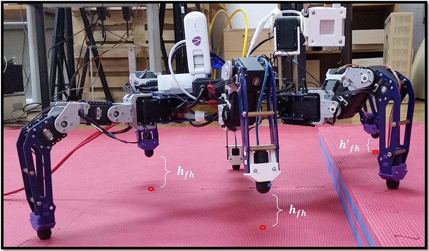
Compared to similar robot designs (e.g. the PhantomX Mark II hexapod robot from Trossen Robotics), the presented hexapod robot structure shown in Figure 1 is modular both component-wise and control-wise. The robot is designed and intended to execute remote commands from an operator, its speed, direction and posture are commanded through a joystick interface, and accordingly, the operator is actively participating in all robot missions. On the other hand, the developed walking algorithm supports the following actions of the robot prototype without any intervention on the part of the operator: Stand-up procedure (e.g. on algorithm start-up). Gait dependant home (reset) procedure in case no instructions for walking are set. While walking, the algorithm respects a preset walking gait while simultaneously making fine adjustments on the gait (e.g. in case of early foot landing due to unexpected ground height). Body roll and pitch control on rough terrain. Local body translation (e.g. for centre of mass correction). Step height and expected ground height correction using a 3D terrain map.

The laboratory prototype of a hexapod robot.
Kinematics
The hexapod robot depicted in Figure 1 belongs to the class of omnidirectional robotic platforms with independent motion of each leg. The robot has six mechanically identical legs

where

Referring to Figure 2 again, the foot frame {Ci} rotates about the z-axis of the knee frame {Ki}, then {Ki} rotates about the z-axis of the hip frame {Hi2}, followed by rotation of the hip frame
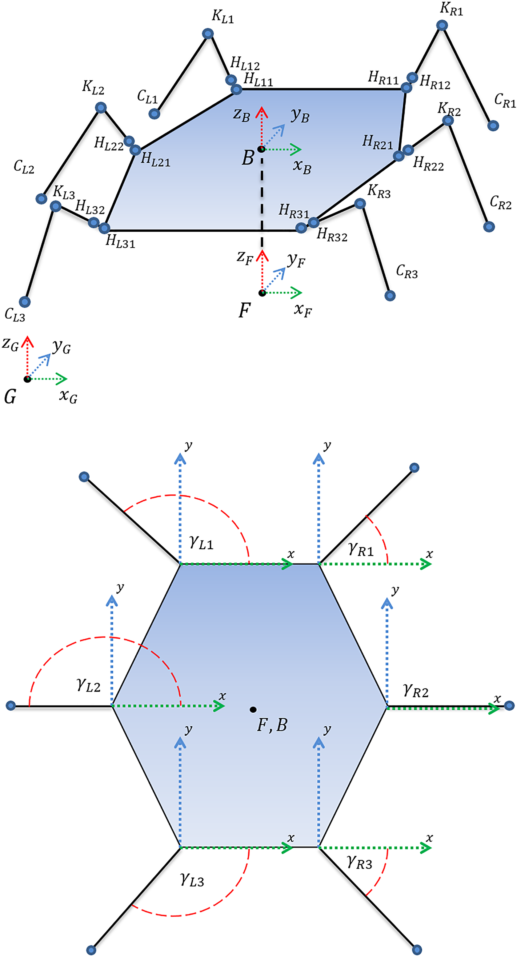
Coordinate systems of a hexapod robot.

Homogeneous transformations used for derivation of a robot kinematics solution.
As all of the robot’s legs have been designed as three-degrees of freedom (3-DOF) mechanisms, they all have the same configuration (i.e. Denavit–Hartenberg parameters) but the distribution of the legs in a hexagonal shape dictates the use of different angular offsets γ i (see Figure 2 and refer to Appendix 2).
The components of the robot’s COB configuration vector

In order to get the values of

where
Each robot leg configuration is identical from the
Circular approximation of robot leg workspaces
Bearing in mind the ultimate objective of conquering uneven terrains, it should be taken into account that very often different legs come into contact with the ground at different heights, directly affecting the sizes of the legs’ respective workspaces and making the trajectory generation problem for each leg much more computationally demanding. In order to effectively cope with the dynamic changes of a leg’s workspace in real time, some simplification of the workspace description becomes a necessity. This workspace description should guarantee no collisions between adjacent legs and should allow for effective trajectory generation in real time. After considering a number of options, we decided upon a circular description.
As shown in Figure 4, by decreasing/increasing the height of the COB, the workspace diameter dwi will become larger/smaller, while the centre cwi will shift further/closer to the origin of frame {F}. Both motion on uneven terrain and motion on even terrain with controlled changes of Circular approximation of robot leg workspace with variations of robot leg workspace in case of different COB heights.

Then, knowing the hip’s angular offset γi for each leg, the values of the centre

Being analytical, the circular approximation provides computationally efficient framework for real-time generation of multiple-leg motion on any type of terrain. This selection of circular workspace approximation will slightly reduce the manoeuvrability of the robot legs, but it is a trade-off necessary for reaching simplicity and computation efficiency in the hexapod robot control system.
Trajectory generation
Solving a trajectory generation problem means needing to resolve how each leg has to move for a given posture of the robot on unpredictable terrain in order to achieve a desired direction of motion. In general, robot motion is determined by a desired longitudinal speed
Figure 5 shows (in green) projections of the robot’s legs’ trajectories onto their circular workspaces for three different manoeuvres executed during the stance phase: moving straight (

Leg trajectory projections (in green) on the leg’s workspaces for moving straight (top left), moving straight-right at
Definition 1
Let a walking robot have n legs in a formation that allows unconstrained motion in the x–y plane. Then, any desired robot motion is composed of equal angular displacements

Interpretation of hexapod robot motion as a composition of individual leg movements along the accompanying circles.
In that sense, the straight motion is a composition of movements of all grounded robot legs along circles of a very large radius. The direction of motion is related to the direction of the centre with respect to {F}. Any other motion along a path with arbitrary curvature can be described, as stated in Definition 1, by composition of individual leg movements along the corresponding circles of finite radii.
Knowing the reference trajectory variables
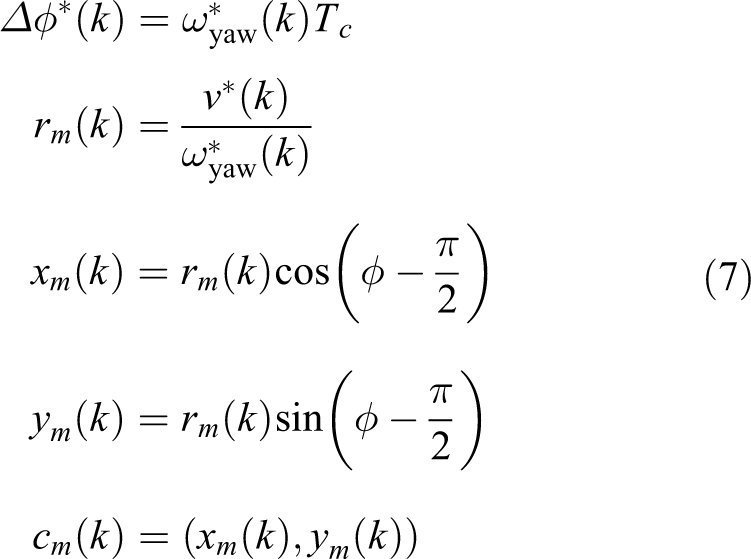
where
Recalling Definition 1, if the grounded legs move on concentric circular trajectories according to the rule
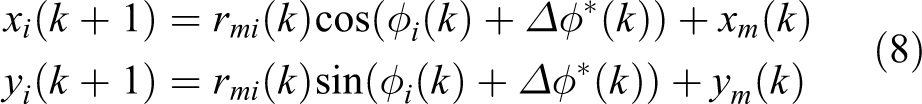
a new desired robot position in the x–y plane with respect to {F} is updated in every control interval Tc as follows

In this way, the trajectory generation problem is redefined as a problem of determining the motion centre
Please note that the described way of calculating individual leg trajectories is applicable to different n-legged designs as stated in Definition 1.
It is obvious that robot motion primarily depends on the legs that are in contact with the ground and which by pushing against the ground contribute simultaneously to translation and rotation of the robot’s COB. In other words, by solving inverse kinematics for each robot leg, generated trajectories for the robot feet along the concentric circles with radii rmj (green curves presented in Figures 5 and 6) are obtained and transformed into required hip and knee movements.
We assume that the stance phase of the robot’s leg stops at the edge of the circular workspace usually referred to as the posterior extreme position (PEP) point. From that position, legs enter into the swing phase and continue moving above the ground in an incremental fashion until reaching the anterior extreme position (AEP) point, that is, touching the ground again (Figure 7) Constraint of stride length by workspace size which varies with footprint position Ci.
As already remarked, the size of the workspace varies in time based on the current footprint position of the robot leg (see Figure 4). Very often robot motion on uneven terrain will cause all legs to have different workspace sizes. This can be countered by always checking the workspace of each robot leg against its present limits.
Mathematically, this can be resolved by knowing the intersection points of the projected trajectory (green curve) and the actual workspace. As shown in Figure 8, the stance and swing intersection points

Check of current leg position on the projected path against stride length limits during robot motion.
Gait control
Executing a certain gait means coordinating all robot legs at the same time. If the hexapod robot is moving on flat terrain, then it can use a tripod gait, ripple gait, wave gait or some modification such as a modified tripod gait. When motion on uneven terrain is considered, the gait control problem becomes more complex. Besides following a given sequence of leg movements in a selected gait, trajectories of each leg must provide smooth motion, including the liftoff and touchdown events. In addition, all legs in the swing phase must be orchestrated in order to be in the right position over the foothold at the right time. As the aim is to have full control of a robot, immediate response must be provided to changes of direction under different translational and rotational speeds. Taking into consideration that the robot could be caught in any posture with its legs poorly positioned for executing a change of walking direction, this is not a trivial planning problem.
Adaptive gait phase control
As mentioned above, movement on uneven terrain will cause legs to land earlier or later than anticipated, thus disturbing the phase sequence of a selected gait, potentially causing the robot to start moving in the wrong direction.
In order to properly tackle this problem, we introduce two new variables,
Regardless of the situation that may occur, we need to know for each leg
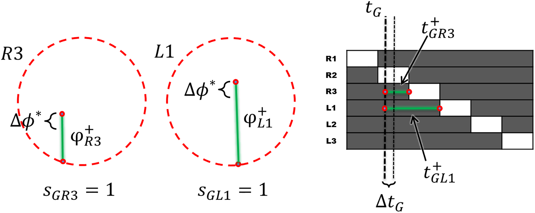
Gait control variables for the wave gait and respective robot legs
Synchronization of legs for a given yaw angle increment
For this purpose, we calculate the ratio between the remaining available workspace (

The obtained number
Step design (introduction of z-component)
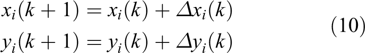
For a given robot motion, the projection of a 3D trajectory on the x–y plane for a grounded leg will always be the same, with only speed and direction along these paths changing. Simultaneously, the legs in the air move incrementally over the x–y plane as defined by equation (10). In order to complete the step design, the leg motion along the z-axis remains to be determined.
One step of a robot leg (see Figure 10) can be divided in three phases: first pushing against the ground (motion from the AEP point ‘1’ to the PEP point ‘2’) corresponding to

Three main phases of a leg step: (1) pushing from the AEP point ‘1’ to the PEP point ‘2’, (2) lifting from the PEP point ‘2’ to the aerial AEP point ‘3’, (3) lowering from the aerial AEP point ‘3’ to the AEP point ‘1’. AEP: anterior extreme position; PEP: posterior extreme position.
Starting with the assumption that the ground is flat, pushing against the ground (the stance phase) occurs at
Stance phase
For a leg in the stance phase, the above-mentioned variable

followed by solving inverse kinematics for each robot leg.
In the case of sudden changes of control variables
Swing phase
For a leg finding itself in an unwanted position in the swing phase, the most important thing is to reach a new AEP point
The displacement of legs in the swing phase is calculated as follows

where
Actual foot coordinates

where PT1 denotes a first-order low-pass filter function.
Once the foot has reached the aerial AEP point straight above the AEP point
Adaptation to uneven terrain
In the previous section, we described the way in which the step of a hexapod robot is designed in order to be able to cope with variations of terrain configuration in a simple way. In the discussion that follows we shall treat different situations the robot may face on uneven terrain as separate control problems to be solved.
Early foot landing
Adaptation to uneven terrain is the robot’s ability to promptly respond to condition
Adaptation of gait execution for the studied situation results in appropriate change of gait variables
Figure 11 shows the example of gait adaptation for early foot landing. Point ‘1’ indicates earlier contact with the ground. The dotted and solid green curves depict a regular step and a step adapted for the case of earlier stepping on the ground, respectively. It should be pointed out that any change of the foot contact height will cause changes in the gait, but the ultimate goal is to get back into the normal gait cycle as soon as the reasons for the step adaptation have ceased to exist. In other words, after one gait cycle

An example of gait adaptation for earlier foot landing.
Ground-level adaptation
Once the leg has landed on the ground, further corrections can be made in addition to the gait adaptation described in the previous subsection. For example, force sensors in the robot’s feet can signal that some of legs are less loaded than others due to uneven terrain, prompting the height of the legs to be adjusted so that force sensor readings of all legs in contact with the ground become equal (see Figure 12). Feet load imbalance may also come from dynamic changes of terrain characteristics in a steady leg contact point

Illustration of ground height estimate
On the other hand, from the implementation point of view, this means that the adjustment algorithm tackles six leg height corrections in the z-direction denoted as
Control of robot body
The described global yaw control can be combined with local robot body control so that a robot can effectively execute its mission. The control goal is to decrease roll and pitch control errors The pitch adjustment relationship of a surf plane, ground surface and a robot.

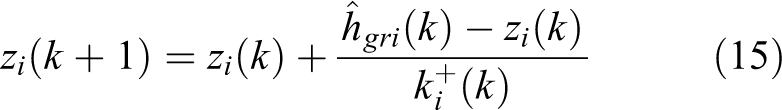
The corrections of z-components (16) are used to update the expected value of ground height

where
Map of terrain-based step adjustment
The described step and posture adaptation of a hexapod robot is retroactive in nature as it relies on acquired feedback information. On the other hand, a proactive approach to step and posture adaptation could be possible if there were to exist a precise 3D map of the environment provided either offline or online before each step is made. Knowing a position in the mapped environment, the robot control system can analyse the terrain and design the next steps of all legs in the desired direction. The trajectories of robot legs can be calculated with respect to the local reference frame {F} which moves along with the robot. The problem to be solved in each control interval is to determine the next foothold location in {F} for the expected robot movement. Figure 14 shows details of how this movement is interpreted and how the prediction of the next foothold position in the x–y plane is made. One can see that while a grounded leg moves towards the next AEP point

Prediction of next foothold position

With the known
Figure 15 shows the side view of foothold height correction from the local reference frame {F} and the respective global reference frame {G}. Care must be taken about the kinematical constraints of the robot which dictate the maximal allowable correction of the foothold height.

View of a foothold height correction with the map of the environment from the local coordinate frame {F} and the respective global coordinate frame {G}.
Balancing the corrections
As most of the corrections of the expected ground height
An example will allow the problem to be explained in more detail. While moving on flat terrain, expected foothold corrections should be close to zero. Supposing now that the expected ground height

An example of balancing the expected ground height adjustments for all robot legs.
Experiments with hexapod robot platform
The described analytically based algorithm for yaw control with all adjustments that allow adaptation of walking gaits on uneven terrains was implemented in the Robot Operating System environment and tested on the hexagonal hexapod robot platform shown in Figure 1. As already mentioned, the driving idea is that the operator issues commands (speed of motion, robot heading and changes of robot posture) to move the robot without thinking over much about the quality of the terrain. For direct locomotion control, the PlayStation 3 DualShock six-axis controller is used, while the Hardkernel WiFi module 3 is used for communication with the computer. The control interval Tc was set to 33 ms.
The robot legs have three electrical actuators, two Dynamixel AX-12A and one Dynamixel AX-18A. The main control unit is an Odroid U3 microcontroller, while a MultiWii MicroWii ATmega32U4 microcontroller executes some auxiliary control functions and acquires force sensor inputs. The Odroid U3 control unit runs on Linux OS. The platform is powered by a Zippy Compact Li-ion battery containing three 3.7 V cells.
Interlink Electronics 0.2″ Circular FSR strain gauges are used for force measurements on all the robot’s legs. Roll and pitch motion of the robot body are measured with an inertial measurement unit InvenSense MPU-6050 (IMU). To be able to add a 3D map of the environment as additional information for adaptive yaw control, a Hokuyo URG-04LX LIDAR sensor is used. The aim of all installed sensors is to enable the robot to walk on varying terrain configurations while keeping its orientation and attitude barely affected.
Laboratory tests showing the hexapod robot in motion are included in the accompanying video supplement.
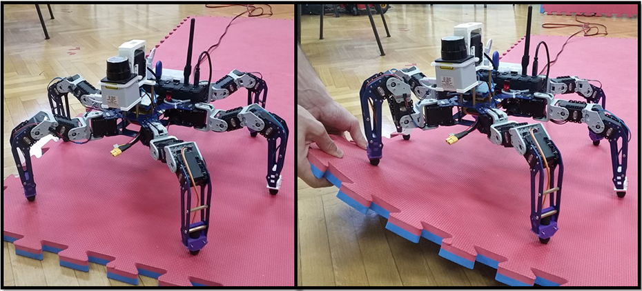
Body control under external disturbances
The robot body control system was tested in a simple way as shown in Figure 17, where the robot was placed standing on the top of a box with constant COB orientation and exposed to manually generated orientation disturbances. The inclusion of the correction algorithm (17) helped the robot to successfully recover a given COB orientation (Figure 18).

Manually generated COB orientation disturbances during testing of the correction algorithm (17).

The responses of the COB roll and pitch control loops under orientation disturbances shown in Figure 17.
Posture adjustment to terrain variations
The robot’s ability to move on uneven terrain is much worse without any adjustment algorithms. For example, the situation with two pairs of robot legs on the ground and one pair in the air may easily cause a tilting effect in case of an imbalance of the robot’s mass. Controlling the yaw angle in this situation is practically impossible. Therefore, the goal of the implemented adjustment is to prevent robot legs staying in the air when they are supposed to be on the ground, resulting in stabilized robot motion as shown in Figure 19. Although the robot does not have perception of the surrounding terrain, by engaging an IMU sensor and the force sensors on its feet it successfully conquers all ground height variations within an expected range of a step height. Even if the robot starts to fall down, it will immediately react to stabilize itself. At the same time, the robot will automatically adjust its posture to sudden variations in terrain configuration as shown in Figure 20.

Stabilized motion of a hexapod robot on the given uneven terrain.
Automatic adjustments of robot posture to sudden variations of terrain configuration.
Control with a 3D map of terrain
It is clear that the quality of robot locomotion on uneven terrain could be much better if a 3D map of terrain was available in advance or acquired online using sensors such as Red-Green-Blue-Depth (RGB-D) cameras and laser sensors. 34,35 Let us now analyse the effects of adding a 3D map with the goal of enabling proactive robot motion planning using acquired information about the terrain on which the robot is moving. For this purpose, a computationally inexpensive Lidar Odometry and Mapping algorithm was implemented. 36
Using the method for predicting the next foothold position (18), the robot becomes capable of accounting for the height of the terrain while adjusting the step heights required to continue walking freely. As shown in Figure 21, knowing the environment enables advance updates of the expected ground height
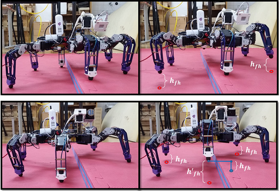
Two examples of advance leg step height planning based on the acquired 3D map of terrain. 3D: three-dimensional.
Another case shown in the lower part of Figure 21 shows that the step heights of legs
Figure 22 shows the leg heights obtained by fusion of 3D map-based and force sensors-based compensations. The former compensation method was active during the swing phase, while the latter came into effect in the stance phase. Both corrections contributed to maintaining the robot’s posture on uneven terrain. This was further enhanced by continuous compensation using equation (17), which led to complete fusion of all compensation mechanisms.

Leg heights obtained after adjustments made by fusion of all compensation algorithms using a 3D map. 3D: three-dimensional.
If we analyse the situation of facing the 4 cm high obstacle without using a map, that is, by using the IMU and force sensors only, then as shown in Figure 23, not being aware of its environment, the robot lifted all its legs equally, touching the ground with its leg

Leg heights during walking over the 4 cm high obstacle without knowledge of the terrain ahead (using only IMU and force sensors). IMU: inertial measurement unit.
The resulting step heights of the robot’s legs during walking on uneven terrain without using a 3D map. 3D: three-dimensional.
The heights of legs shown in Figure 23 are the result of several adjustments going on in parallel. Here it is convenient to analyse the responses of expected ground heights

The expected ground heights for robot legs during walking over the 4 cm high obstacle without knowledge of the terrain ahead (using only IMU and force sensors). IMU: inertial measurement unit.
Besides the main algorithm, also active here is a slower compensation mechanism responsible for balancing expected ground height corrections. This becomes noticeable every time an earlier landing of a leg occurred. In those moments, the average ground height of all legs gets higher, and balancing tends to decrease this average value to zero. This balancing effect (lowering the leg heights) can be clearly seen in the responses of leg heights shown in Figure 23 and expected ground height in Figure 25.
Walking over the 4 cm high obstacle without a map noticeably affects the robot’s orientation. One can see in Figure 26 that the correction algorithm (17) successfully compensated these disturbances and reduced roll and pitch angle deviations to zero.

Compensation of COB orientation disturbances while overcoming a 4 cm high obstacle without knowledge of the terrain ahead (using only IMU and force sensors). IMU: inertial measurement unit.
Conclusion
The analytically founded adaptive yaw control algorithm devised in this work enables a legged robot to continuously adapt its walk on uneven terrain. The circular approximation of leg workspace makes control of a robot easier and computationally more efficient in all situations. Regarding the method of motion generation for the robot legs, the original concept of calculating concentric circular trajectories around an analytically determined motion centre is proposed. This systematic motion model allowed easy generation of smooth, synchronized motions for all robot legs. The gait synchronization is realized by introducing new adaptable gait control variables related to the detected moments of leg liftoff and touchdown. With this new analytically based adaptive gait control it became possible to change the gait during robot motion, and fuse and balance a number of additional corrections that adapt the legged robot locomotion to the ground.
Although the proposed control algorithm was developed to the point where the robot could overcome the basic unevenness of terrain and was able to keep direction, there is a lot of potential for further improvement. One of the most effective enhancements would be adding compliance to robot motion, as well as more agile walking and running gaits, which will certainly bring new control issues and further progress in these directions. Future tests performed on natural terrains will help to fully objectively evaluate this new walking gait control method. Comparative analysis of the proposed analytically based adaptive yaw control method to other control approaches in literature will provide answers regarding the method’s applicative value. Also, we plan to test the practical applicability of the method to other types of walking robots. Quadruped robots that are less stable than hexapod robots are seen as prime candidates for the implementation of the proposed control approach. 37 –39
Footnotes
Acknowledgments
The authors want to acknowledge contributions of Luka’s colleagues Antun and Josip Vukičević during the design and experimental phases presented in this work.
Declaration of conflicting interests
The author(s) declared no potential conflicts of interest with respect to the research, authorship, and/or publication of this article.
Funding
The author(s) received no financial support for the research, authorship, and/or publication of this article.
Appendix A
Homogeneous transformation from the hip frame {Hi1} to the local reference frame {F}.
where Cx = cosx, Sx = sin x.
Appendix 2
Hexapod robot dimensions and D-H kinematic parameters of a robot leg (a1 = 5.2 cm, a2 = 6.56 cm, a3 = 13.81 cm) (Figure 2A).
Appendix 3
Inverse kinematics of a hexapod robot leg
where a1, a2, and a3 denote lengths of the legs’ links and x, y, and z represent coordinates of {Ci} expressed in {Hi1}.
References
Supplementary Material
Please find the following supplemental material available below.
For Open Access articles published under a Creative Commons License, all supplemental material carries the same license as the article it is associated with.
For non-Open Access articles published, all supplemental material carries a non-exclusive license, and permission requests for re-use of supplemental material or any part of supplemental material shall be sent directly to the copyright owner as specified in the copyright notice associated with the article.