Sage Journals: Discover world-class research

Abstract

Nowadays, the usage of autonomous mobile robots that fulfill various activities in enormous number of applications without human’s interference in a dynamic environment are thriving. A dynamic environment is the robot’s environment which is comprised of some static obstacles as well as several movable obstacles that their quantity and location change randomly through the time. Efficient path planning is one the significant necessities of these kind of robots to do their tasks effectively. Mobile robot path planning in a dynamic environment is finding a shortest possible path from an arbitrary starting point toward a desired goal point which needs to be safe (obstacle avoidance) and smooth as well as possible. To achieve this target, simultaneously satisfying a collection of certain constraints including the shortest, smooth, and collision free path is required. Therefore, this issue can be considered as an optimization problem, consequently solved via optimization algorithms. In this article, a new method based on cuckoo optimization algorithm is proposed for solving the mobile robot path planning problem in a dynamic environment. Furthermore, to diminish the computational complexity, the feature vector is also optimized (i.e. reduced in dimension) via a new proposed technique. The simulation results show the performance of proposed algorithm in finding a short, safe, smooth, and collision free path in different environment conditions.

Keywords

Autonomous mobile robot path planning cuckoo optimization algorithm dynamic environment

Introduction

In the modern era, a variety of different aspects of human life have been involved in using intelligent machines that are able to do various activities in dynamic environments. Among them, autonomous mobile robots have been taken into consideration by researchers in last decades. These robots are used in plenty of various activities including human assistant in daily life, working in high-level dangerous environments, fulfilling impossible tasks for human (e.g. exploration in space and discovery operations). Therefore, they need to directly extract information from their surroundings without human interferes, move within the environment, make decision, and finally perform their tasks safely, meaningfully, and independently using the knowledge they already gained. In addition, moving through the environment is the most crucial and fundamental feature they need to possess. Hence, finding an optimum (the shortest, safe and smooth) path from an arbitrary starting point toward the goal point is considered as one of their basic requirements.^1,2

In the autonomous mobile robot path planning research field, there are three kinds of different environments: static environment with fixed obstacles, dynamic environment with movable obstacles, and also dynamic environment with movable obstacles and the target point simultaneously. Dynamic environment is an unknown environment which has several portable obstacles that move at the same time with robot all around the space with random direction, velocity, and speed. It also might include some static obstacles as well (e.g. walls, doors, furniture, etc.).³

Mobile robots path planning research field commenced in the middle of 1960s. At the beginning, researchers worked on static environments and used statistical and mathematical methods such as Artificial Potential Field^1–5 and Visibility Graph to solve the problem. Although these kinds of methods were able to find sufficient paths, they had some natural drawbacks including getting stuck into local minimum, lack of enough margin from obstacles, oscillations in the face of obstacles and narrow passages.

Recently, research on artificial intelligence has flourished rapidly, and many intelligent algorithms have been applied to the mobile robot path planning problem such as artificial neural network (ANN), fuzzy logic (FL), genetic algorithms (GA), particle swarm optimization (PSO), ant colony optimization (ACO), bee colony optimization (BCO), and also hybrid methods. Pandey et al. introduced the literature survey of the various algorithms used for mobile robot navigation.⁴ They classified the algorithms for solving the mobile robot navigation problem into three categories: (1) deterministic algorithms (fuzzy logic, neural network, neuro fuzzy), (2) nondeterministic algorithms (GA, PSO, Simulated Annealing (SA), ANT colony), and (3) evolutionary algorithms (fuzzy + nondeterministic algorithm, neural network + nondeterministic algorithm). In Table 1, we summarize a number of different methods used by researchers to solve the mobile robot path planning problem.

Table 1.

Summary of different methods developed in path planning problem.

	Environment
		Dynamic
Method	Static	Only obstacles	Target and obstacles
Artificial potential fields
Khatib,⁵	▄	▄
Sharir,⁶	▄	▄
Hou and Zheng,⁷	▄
Conkur,⁸	▄
Malone et al.⁹	▄	▄
ANN
Christopher Kazakiewicz, Masakazu	▄
Glasius et al.¹⁰	▄	▄
Yang and Meng,¹¹	▄	▄	▄
Bin et al.¹²	▄	▄
Willms and Simon,¹³	▄	▄	▄
Qu et al.¹⁴	▄	▄	▄
FS
Surmann et al.¹⁵	▄
Lei and Li,¹⁶	▄	▄
Woo and Polisetty,¹⁷	▄		▄
Mobadersany et al.¹⁸	▄	▄
Sun and Yu,¹⁹	▄
Pandey and Parhi,²⁰	▄	▄
ACO
Fan et al.²¹
Tan et al.²²	▄
WooLee et al.²³	▄
Brand et al.²⁴	▄
Zhang et al.²⁵	▄	▄
PSO
Nasrollahy and Javadi,²⁶	▄	▄	▄
Zhao and Zu,²⁷	▄	▄
Masehian and Sedighizadeh,²⁸	▄	▄
Shakiba et al.²⁹	▄	▄	▄
Lee et al.³⁰	▄
Artificial bee colony
Saffari and Mahjoob,³¹	▄
Ma and Lei,³²	▄	▄
Goel and Singh,³³	▄	▄
Mansury et al.³⁴	▄	▄	▄
Darwish et al.³⁵	▄	▄
GA
Sedighi et al.³	▄	▄
Shi and Cui,³⁶	▄	▄
Chuan-Ling et al.³⁷	▄	▄
Tsai et al.³⁸	▄
Roberge et al.³⁹	▄
Hybrid methods
Juidette and Youlal,⁴⁰ (GA + FS)	▄	▄
Aydin and Temeltas,⁴¹ (DE + FS)	▄
Xin et al.⁴² (GA + NN)	▄
Porta García et al.⁴³ (ACO + fuzzy fitness function)	▄	▄
Jaradat et al.⁴⁴ (fuzzy potential field)	▄	▄	▄
Xue and Jian-Qiao,⁴⁵ (multi-objective evolutionary algorithm)	▄

ANN: artificial neural network; GA: genetic algorithm; ACO: ant colony optimization; FS: fuzzy system; PSO: particle swarm optimization; DE: Differential Evolution.

In this article, we introduce an algorithm for solving the mobile robot path planning problem. The objective of this research is to find a short, safe, and smooth path collision avoidance for mobile robot path planning in dynamic environment and diminish the computational complexity.

Cuckoo optimization algorithm

Cuckoo optimization algorithm (COA)⁴⁶ was introduced for solving nonlinear optimization problems in continuous space by Ramin Rajabioun which is inspired by cuckoo’s life style. Cuckoos, on the contrary of other birds, don’t make nest for themselves and always use other bird’s nest to reproduce. Similar to any population-based algorithms, COA starts with an initial population of mature cuckoos. This population, lay some eggs in different nests. Those eggs that have more similarities to the host bird’s eggs have more chance to grow and become a mature cuckoo, whereas, the rest of them that are identified by the host birds will be obliterated. Afterward, the rate of the grown eggs reveals the proper nests for laying among all areas. In other word, the more grown eggs in an area, the more suitable conditions for laying eggs there. When the eggs grow up and become mature cuckoos, they make several societies and each society has its own habitat region. Then, the best habitat region among these societies is considered as the other cuckoo’s destination for immigration; they immigrate and reside in a place near the best habitat region. Afterward, cuckoos start laying in random nests that are located in their laying radius. This process continues until the best area is found. Figure 1 shows the COA flowchart.

Figure 1.

COA flowchart.⁴⁶ COA: cuckoo optimization algorithm.

Assumptions

In this article, a new approach is presented to solve the dynamic path planning problem for autonomous mobile robots. Since finding a path in a dynamic environment requires satisfying several distinct and certain constraints, the problem is considered as an optimization problem. Afterward, for solving this optimization problem a new method based on COA is defined. There are several assumptions that are considered as follows:

The robot works in a 2-D environment, which is represented by a 2-D matrix.

Obstacles in environment are defined as polygon shapes. The number and size of obstacles are randomly generated inside the environment.

The size of the robot is equivalent to one grid network cell.

The robot and obstacles move in every possible direction in the grid network—eight possible directions.

The velocity of robot is constant and equals to exactly one cell per step in any eight possible direction. Therefore, the average speed of robot is one cell per step.

The speed of obstacles is random and based on the equation (1), which is always either 0 or 1 cell per step (i.e. equal or smaller than the speed of the robot).

Speed (x) = {\begin{cases} 0, | x < 0.5 \\ 1, | x \geq 0.5 \end{cases}

where x is a random number based on uniform probability distribution. It is worthy of emphasize: x is separately generated for any single individual obstacle at any step and, consequently, the speed function is run for determining any obstacle’s speed independently.

Proposed algorithm

According to the dynamic environment, the proposed algorithm is executed step-by-step and online. The shortest path between two arbitrary points, presumably, is the straight line between these two points. Therefore, our algorithm picks this line (i.e. the straight line between the start and the goal points) as the reference line (L _R). Then, some points are dynamically chosen on this line and considered as feature vector (optimization variables). Afterward, in each step, the COA is run once and the best-found solution is known as the best path for the current step. After that, the robot moves toward the first point (P ₁) in the calculated path, after the robot reaches P ₁, this point is considered as the new starting point (P _s). Thereupon, this operation continues until the robot reaches the goal point (P _g). In other words, when P _s = P _g, the robot reached the goal point and the algorithm will stop. Flowchart of the proposed algorithm is shown in Figure 2, and the algorithm itself is presented as Algorithm 1.

Figure 2.

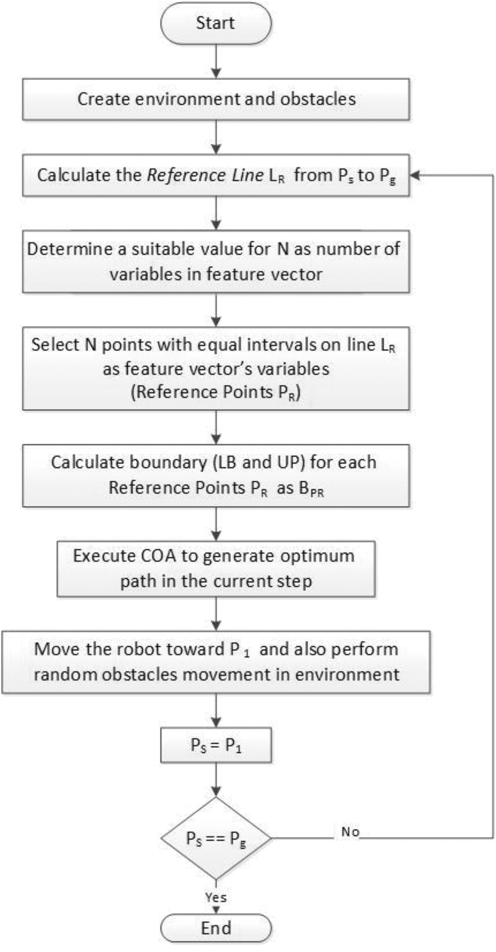
Proposed algorithm flowchart. COA: cuckoo optimization algorithm.

Algorithm 1.

Proposed algorithm.

Calculate the straight line between the start and the goal points, named reference line as L _R.

Choose a suitable number of points (N) on L _R as the total number of variables in feature vector.

Select N points with equal intervals on L _R as feature vector that is shown via P _R as reference points.

Calculate upper and lower bound for all points in P _R and keep them in reference points Boundary matrix showed by BP _R.

Execute COA in order to find optimum path in the current step.

Move robot toward the first point (P ₁) in calculated optimum path.

Replace the start point with the first point that robot has just moved there (P _s = P ₁).

If P _s ≠ P _g then, move the obstacles randomly and go to I; otherwise stop the algorithm.

Reference line (L _R)

The reference line (L _R) is the straight line between P _s and P _g. In fact, L _R is ideally the shortest possible path between P _s and P _g. Moreover, the optimal path is aimed to be generated as much as near the L _R. Therefore, in the best case (no obstacle collides the L _R), the optimal path is the L _R itself as it is shown in Figure 3.

Figure 3.

Reference line L _R and reference points P _R.

Feature vector

Given the definition of problem, the aim of the algorithm is to find a set of consecutive points in a 2-D space and make a path between two arbitrary points by connecting these points together; therefore, these points are considered as the feature vector. Moreover, due to the inevitable impact of the number of feature vector’s variables (N) on algorithm’s performance, it needs to be calculated dynamically. Selecting a constant value for N, instead, leads to ignore the environment’s dynamic condition (e.g. the number of obstacles, the length of L _R and obstacles’ distance through L _R) which eventually affects the algorithm’s performance in the converge speed and accuracy as well. In the proposed algorithm, the value of N is calculated dynamically based on the environment’s conditions as shown in equation (2).

N = (\frac{d}{4}) + (C_{N} \times 2)

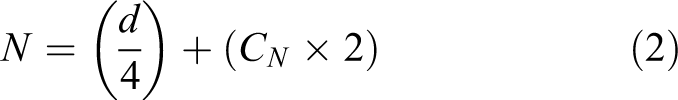
where d denotes the Euclidean distance between the start and the goal points, and C_N is the number of obstacles that L _R crosses them. After choosing a suitable value for N, the idea is to find a set of N consecutive points (i.e. starting from P _s and finishing at P _g) and link them together to generate a path. In this article, a new technique is proposed for reducing the search space dimension. In our technique, 2-D feature vector is mapped to 1-D; as a result, the search space is circumscribed. Consequently, by reducing the search space as well as the feature vector’s dimension, not only the computational complexity will be reduced but also the execution time will meaningfully be improved. In our approach, instead of using 2-D coordinate of points $P_{i} = [\begin{matrix} X_{i} \\ Y_{i} \end{matrix}]$ , the perpendicular distance of these points from reference points (P _R) is used as feature vector. Reference points (P _R) are composed of N consecutive points with equal intervals on L _R as shown in Figure 3.

As a result, the perpendicular distance of each points from their corresponding reference points $S, P_{R 1}, P_{R 2}, \dots, G$ are considered as the feature vector rather than the coordinates of points $S, P_{1}, P_{2}, \dots, G$ . Note that all points ( $P_{1}, P_{2}, \dots, P_{N}$ ) can only be located on perpendicular line on their corresponding reference points; therefore, the distance between points P_i and its corresponding reference point $P_{R i}$ is equal to perpendicular distance on L _R at point $P_{R i}$ . Figure 4 demonstrates the process carefully.

Figure 4.

Calculating distance between points P_i and $P_{R i}$ on $L_{R}$ .

The feature vector of the path in Figure 4 is explained in Table 2 that are only the perpendicular distance of each points to their corresponding P _R on L _R. This feature vector, afterward, fed to COA as a habitat.

Table 2.

An example of a 1-D feature vector based on Figure 4.

$P_{R}$	$P_{R 1}$	$P_{R 2}$	$P_{R 3}$	$P_{R 4}$	$P_{R 5}$	$P_{R 6}$	$P_{R 7}$	$P_{R 8}$	$P_{R 9}$	$P_{R 10}$	$P_{R 11}$
Values	4.5	∞	6	−1.5	∞	−6.5	3	2	2.5	−1	−3

Execute COA

The proposed algorithm uses COA to optimize the mentioned distances by considering the upper and lower bound of each reference points. Bear in mind, the value ∞ shows that there is no point on the perpendicular line on the reference point $P_{R i}$ , and this point will be omitted practically from the path. Consequently, to generate the path, the previous point $P_{R i - 1}$ is connected to the next point $P_{R i + 1}$ . It happens when an unacceptable value for the point is generated (i.e. the value is out of the range of [UB LB] for $P_{R i}$ ) during either migration or laying process in the COA. For example, as shown in Figure 4, there is no point on perpendicular line on reference point $P_{R 2}$ , so the point P ₁ is directly connected to the point P ₃. Note that, in our approach of dimensional reduction, a large part of search space is not reachable at each step. Therefore, the robot cannot explore those areas. But given the fact that the robot always decides for the next step at any time, after moving toward P ₁ and replacing this point with $P_{s}$ , a new reference line—with a different line slope—is generated. As a result, a different part of search area is explored.

Fitness function

Given the fact that the mobile robot path planning problem is considered as a minimization problem, first, the cost function and, then the fitness function is defined. Since the optimal path should be short, smooth, safe, and also obstacle avoidance, the cost function is composed of four subfunctions as below. Bear in mind, in all following subfunctions, N represents the number of points that forms the whole path (the whole path is formed by $n - 1$ subpath).

1. Smoothness subfunction:

A smooth path is a path that the angle between any two consecutive sublines (which formed a part of the path) be high enough not to force the robot to change its movement suddenly with a steep angle. Equation (3) shows the smoothness subfunction

f_{s} = \sum_{i = 1}^{N - 1} α (l_{i}, l_{i + 1})

where $α (l_{i}, l_{i + 1})$ is the angle between lines l_i and $l_{i + 1}$ and also $f_{s}$ represents the degree of the smoothness.

2. Length subfunction:

The length subfunction is calculated by equation (4) based on Euclidean distance method

f_{l} = \sum_{i = 1}^{N - 1} \sqrt{{(x_{i + 1} - x_{i})}^{2} + {(y_{i + 1} - y_{i})}^{2}}

where x_i and y_i represent the coordinate of point i.

3. Safety subfunction:

A safe path is as far as possible from the obstacles. In other word, the path would be generated with a safe distance from obstacles. Equation (5) demonstrates the safety subfunction.

f_{r} = \sum_{i = 1}^{N - 1} D_{L i}

where $D_{L i}$ denotes the minimum distance of line L_i (ith subpath) from all obstacles in environment.

4. Collision-free subfunction:

This subfunction is designed to detect and punish unreachable (infeasible) path that has at least one collision and is defined by equation (6)

f_{c} = \sum_{i = 1}^{n - 1} C_{L i}

where $C_{L_{i}}$ represents the number of collisions of ith subpath.

Finally, the cost function is defined as shown in equation (7)

F_{cost} = (\frac{w_{1}}{f_{s}}) + (w_{2} \times f_{l}) + (\frac{w_{3}}{f_{r}}) + (w_{4} \times f_{c})

where w ₁, w ₂, w ₃, and w ₄ are the coefficients of smoothness, length, safety, and collision-free subfunctions, respectively. The way that these coefficients are multiplied to their related subfunctions shows that the smoothness sub-function, as well as the safety subfunction, ought to be maximized; on the other hand, the length and collision-free subfunctions should be minimized. Therefore, different coefficients will generate different paths (e.g. if the safety coefficient (w3) is considered too high, then the safest path will be generated instead of the shortest one). Afterward, the fitness function for COA in the proposed algorithm is defined as equation (8)

Profit = - F_{cost} = - [(\frac{w_{1}}{f_{s}}) + (w_{2} \times f_{l}) + (\frac{w_{3}}{f_{r}}) + (w_{4} \times f_{c})]

Furthermore, from the time complexity perspective, the complex cost function of the proposed algorithm—that is presented in equation (7)—needs to get optimized through a fast optimization algorithm. Therefore, among all the novel optimization algorithms (e.g. GA, BCO, ACO, and PSO) the COA was chosen due to its great ability of finding better solutions in fewer iterations than GA and PSO, as described in the simulation results of the original article of the COA.⁴⁶

Movement modeling

COA is executed for finding the best path in each step, after finding one, the robot moves toward the first point (P ₁) in the generated path. To calculate the exact coordinate of point P ₁, first of all, the value of $P_{R 1}$ —which represents the perpendicular distance between point P ₁ and the reference point $P_{R 1}$ on line $L_{R}$ —is calculated. Then, the coordinate of $P_{1} = [\begin{matrix} X_{1} \\ Y_{1} \end{matrix}]$ is extracted using the reference line ( $L_{R}$ ), the perpendicular line on $L_{R}$ at reference point $P_{R 1}$ , points $P_{R 1}$ , $P_{s}$ , $P_{g}$ , and also, the distance between point P ₁ and point $P_{R 1}$ . The procedure of calculating the exact coordinate of point P ₁ is shown in Figure 5.

Figure 5.

Calculating the exact coordinate of point P ₁.

After calculating the exact coordinate of point P ₁, the robot moves toward it while all obstacles move with random speed and directions simultaneously. In this circumstance, there is a probability of collision between the robot and obstacles. To prevent this unwilling accident, first, the number of required step points for robot to reach the point P ₁ is calculated, then, the exact coordinate of each step-points is obtained. Finally, if and only if there is no obstacle in the unicellular radius from the first step-point exists, then robot performs the first step; otherwise, robot cannot accept the collision risk and rejects the path (i.e. COA runs again for finding another feasible path). This process continues for each step-points until robot reaches the point $P_{1}$ . Note that, in case of rejecting the path, robot’s current position is considered as new $P_{s}$ .Figure 6 shows this process.

Figure 6.

Moving the robot toward point P ₁.

Although, theoretically, in a crowded environment, the robot might have collision while moving toward P ₁, the simulation results has shown the probability of this collision is substantially low. Moreover, another subfunction can be defined in the cost function to prevent any possible collisions through robot movement toward point P_i , which leads to increase the computational cost.

Simulation results

The simulation results show the performance and the power of proposed algorithm to find a short, safe, collision free (as far as possible from obstacles) path. Bear in mind, any changes in corresponding coefficients of four subfunctions in fitness function in equation (7) will affect the algorithm’s performance and how the path is generated (i.e. described in “Feature vector” section). All experimental results are based on coefficients shown in Table 3, which is obtained by trial and error manner, in which the collision-free subfunction is more important than the length subfunction. In the following, the result of the proposed algorithm is shown in small, medium, and large environments, in which their size is 20 × 20 cm², 100 × 100 cm², and 200 × 200 cm², respectively. Figures 7 and 8 represent the generated path in small environment with two and four dynamic obstacles, respectively. Furthermore, Figures 9 and 10 show the generated path in medium environment that is comprised of 10 and 20 dynamic obstacles, respectively. Finally, Figure 11 shows the algorithm’s performance to find the optimum path in large environment with 20 dynamic obstacles.

Table 3.

Value of coefficients of fitness function’s subfunctions in simulation.

Coefficient	Value	Description
w ₁	2	Smoothness subfunction
w ₂	8	Length subfunction
w ₃	2	Safety subfunction
w ₄	16	Collision-free subfunction

Figure 7.

Result of proposed algorithm in the small environment with two dynamic obstacles: (a) initialize setting; (b) roughly 1/3 of the generated path; (c) roughly 2/3 of the generated path; and (d) the whole generated path.

Figure 8.

Result of proposed algorithm in the small environment including four dynamic obstacles: (a) initialize setting; (b) roughly 1/3 of the generated path; (c) roughly 2/3 of the generated path; and (d) the whole generated path.

Figure 9.

Result of proposed algorithm in the medium environment comprised of 10 dynamic obstacles: (a) initialize setting; (b) roughly 1/3 of the generated path; (c) roughly 2/3 of the generated path; and (d) the whole generated path.

Figure 10.

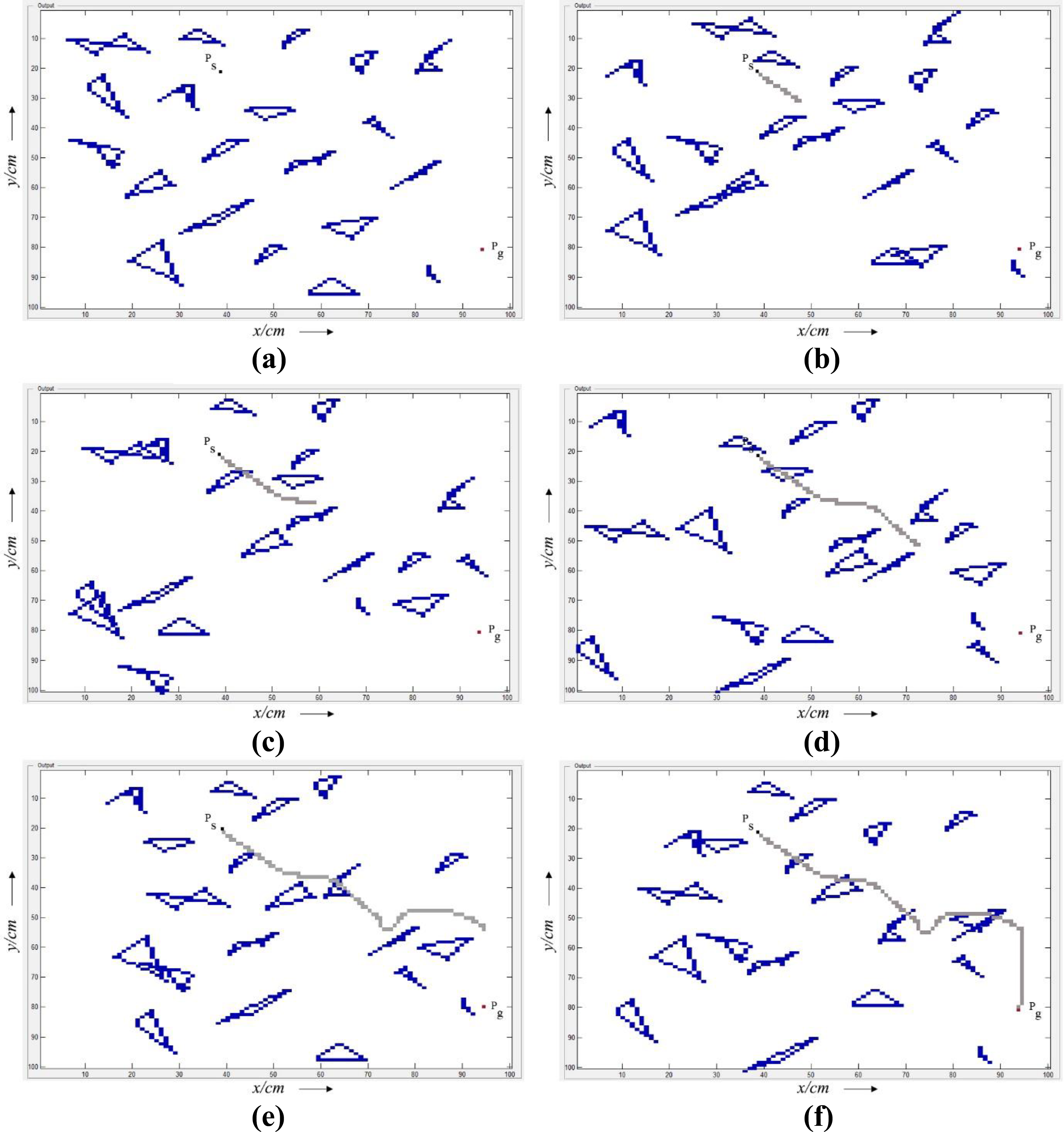
Result of proposed algorithm in the medium environment with 20 dynamic obstacles: (a) initialize setting; (b) roughly 1/5 of the generated path; (c) roughly 2/5 of the generated path; (d) roughly 3/5 of the generated path; (e) roughly 4/5 of the generated path; and (f) the whole generated path.

Figure 11.

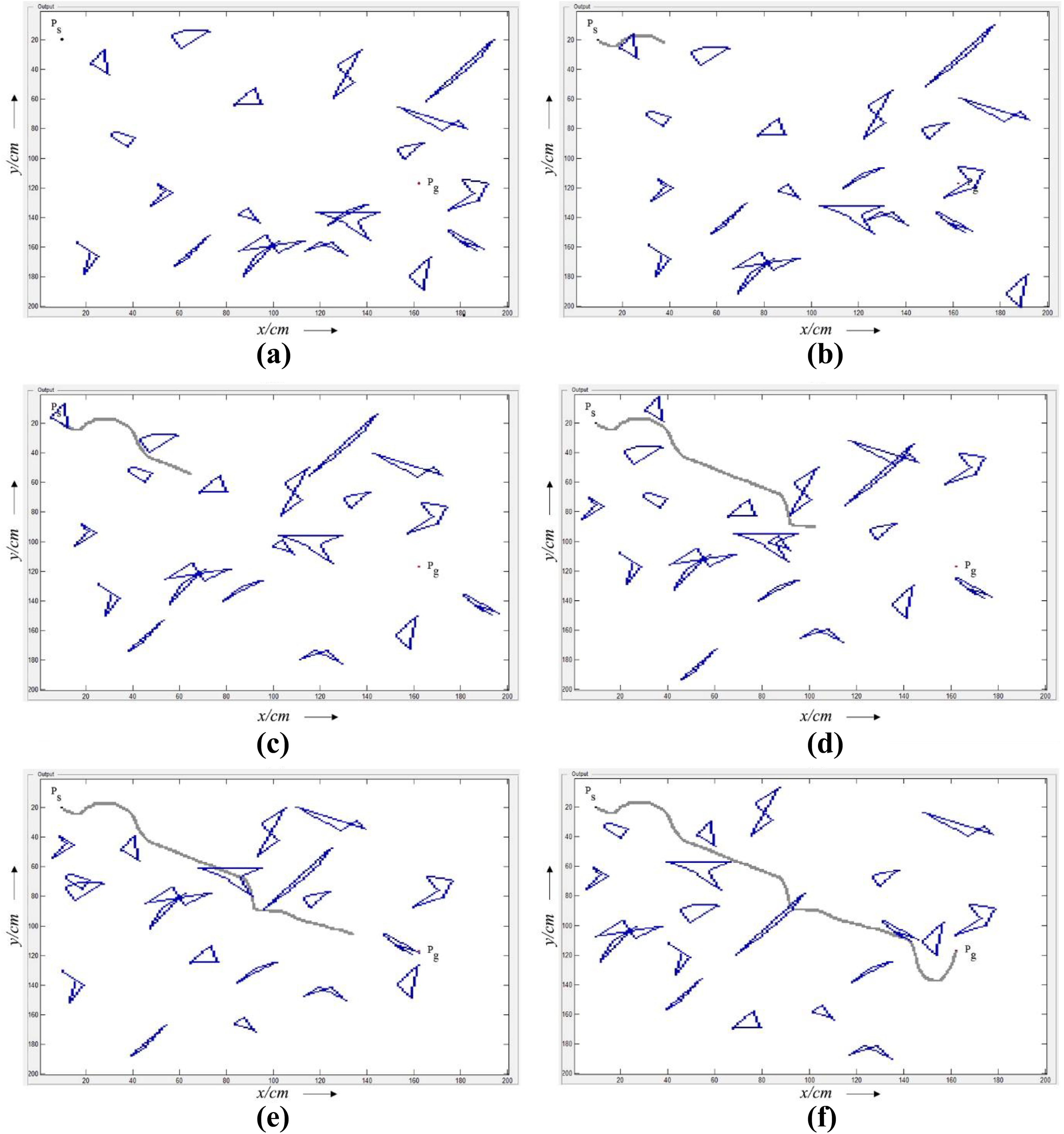
Result of proposed algorithm in the large environment which has 20 dynamic obstacles: (a) initialize setting; (b) roughly 1/5 of the generated path; (c) roughly 2/5 of the generated path; (d) roughly 3/5 of the generated path; (e) roughly 4/5 of the generated path; (f) the whole generated path.

Note that, in the following figures, the black, red, blue, and gray cells are the start point, goal point, obstacles, and robot path by the time, respectively.

Conclusion

In the modern era, autonomous mobile robots, which work in a dynamic environment that is composed of several static and movable obstacles, play a vital rule in many aspects of daily life from industry to human-aid usage. The foundation of fulfilling their tasks is to find the efficient path between two arbitrary points to move through the dynamic environment effectively. Therefore, mobile robot path planning is to finding a shortest possible path between two points, which also needs to be safe (i.e. no collision with any obstacle) and smooth as well. In this article, a new method based on COA has been formed for solving the mobile robot path planning problem in a dynamic environment—comprised of several static and movable obstacles in different random polygon shapes. Plus, a new technique has been proposed to reduce the feature vector’s dimension (i.e. mapping 2-D matrix to 1-D vector) to overcome the overall computational complexity. The simulation results show the performance and power of proposed algorithm in generating a short, safe, smooth, and collision-free path in different environmental conditions. For our future trend, we will extend our method in a dynamic environment with a movable goal point, which is considered as complex as the real-world environment.

Footnotes

Declaration of conflicting interests

The author(s) declared no potential conflicts of interest with respect to the research, authorship, and/or publication of this article.

Funding

The author(s) received no financial support for the research, authorship, and/or publication of this article.

ORCID iD

Chitra Dadkhah

References

Katić

Vukobratović

. Survey of intelligent control techniques for humanoid robots. J Intell Robot Syst 2003; 37(2): 117–141.

Goodrich

Schultz

. Human–robot interaction: a survey. Found Trends® Hum Comput Interact 2008; 1(3): 203–275.

Sedighi

Ashenayi

Manikas

. Autonomous local path planning for a mobile robot using a genetic algorithm. In: Congress on evolutionary computation, 2004. CEC2004, Portland, OR, USA, 19–23 June 2004.

Pandey

. Mobile robot navigation and obstacle avoidance techniques: a review. Int Robot Autom J 2017; 2(3): 00022.

Khatib

. Real-time obstacle avoidance for manipulators and mobile robots. Int J Robot Res 1986; 5(1): 90–98.

Sharir

. Algorithmic motion planning in robotics. Computer 1989; 22(3): 9–19.

Hou

Zheng

. Mobile robot path planning based on hierarchical hexagonal decomposition and artificial potential fields. J Robotic Syst 1994; 11(7): 605–614.

Conkur

. Path planning using potential fields for highly redundant manipulators. Robot Auton Syst 2005; 52(2): 209–228.

Malone

Chiang

H-T

Lesser

. Hybrid dynamic moving obstacle avoidance using a stochastic reachable set-based potential field. IEEE Trans Robot 2017; 33(5): 1124–1138.

10.

Glasius

Komoda

Gielen

. Neural network dynamics for path planning and obstacle avoidance. Neural Networks 1995; 8(1): 125–133.

11.

Yang

Meng

. Real-time collision-free path planning of robot manipulators using neural network approaches. Auton Robot 2000; 9(1): 27–39.

12.

Bin

Xiong

Liming

. Recurrent neural network for robot path planning. Lect Notes Comput Sci 2005; 3320: 188–191.

13.

Willms

Simon

. Real-time robot path planning via a distance-propagating dynamic system with obstacle clearance. IEEE Trans Syst Man Cybern B 2008; 38(3): 884–893.

14.

Yang

Willms

. Real-time robot path planning based on a modified pulse-coupled neural network model. IEEE Trans Neural Netw 2009; 20(11): 1724–1739.

15.

Surmann

Huser

Wehking

. Path planning far a fuzzy controlled autonomous mobile robot. In: Proceedings of the fifth IEEE international conference on Fuzzy Systems, 1996, New Orleans, LA, 8–11 September 1996.

16.

Lei

. A fuzzy behaviours fusion algorithm for mobile robot real-time path planning in unknown environment. In: IEEE international conference on integration technology, 2007. ICIT ‘07, Shenzhen, 20–24 March 2007.

17.

Woo

P-Y

Polisetty

. ANFIS generated dynamic path planning for a mobile robot to track a randomly. In: 2010 IEEE international conference on fuzzy systems (FUZZ), Barcelona, 18–23 July 2010.

18.

Mobadersany

Khanmohammadi

Ghaemi

. An efficient fuzzy method for path planning a robot in complex environments. In: 21st Iranian conference on electrical engineering (ICEE), 2013, Mashhad, 14–16 May 2013.

19.

Sun

. Tracking control for a cushion robot based on fuzzy path planning with safe angular velocity. IEEE/CAA J Automatica Sinica 2017; 4(4): 610–619.

20.

Pandey

Parhi

. Optimum path planning of mobile robot in unknown static and dynamic environments using Fuzzy-Wind Driven Optimization algorithm. Def Technol 2017; 13(1): 47–58.

21.

Fan

Luo

. Optimal path planning for mobile robots based on intensified ant colony optimization algorithm. In: IEEE international conference on robotics, intelligent systems and signal processing, 2003, Changsha, Hunan, China, 8–13 October 2003.

22.

Tan

Huan

Aaron

. Ant colony system algorithm for real-time globally optimal path planning of mobile robots. Acta Automatica Sinica 2007; 33(3): 279–285.

23.

WooLee

JungKim

SukChoi

. Improved ant colony optimization algorithm by potential field concept for optimal path planning. In: 8th IEEE-RAS international conference on humanoid robots, 2008. Humanoids 2008, Daejeon, 1–3 December 2008.

24.

Brand

Masuda

Wehner

. Ant colony optimization algorithm for robot path planning. In: 2010 International conference on computer design and applications (ICCDA), Qinhuangdao, 25–27 June 2010.

25.

Zhang

Gong

Han

. An improved ant colony algorithm for path planning in one scenic area with many spots. IEEE Access 2017; 5: 13260–13269.

26.

Nasrollahy

Javadi

HHS

. Using particle swarm optimization for robot path planning in dynamic environments with moving obstacles and target. In: Third UKSim European symposium on computer modeling and simulation, 2009. EMS ‘09, Athens, 25–27 November 2009.

27.

Zhao

. Real-time obstacle avoidance method for mobile robots based on a modified particle swarm optimization. In: International joint conference on computational sciences and optimization, 2009. CSO 2009, Sanya, Hainan, 24–26 April 2009.

28.

Masehian

Sedighizadeh

. A multi-objective PSO-based algorithm for robot path planning. In: 2010 IEEE international conference on industrial technology (ICIT), Vi a del, 14–17 Mar 2010.

29.

Shakiba

Najafipour

Salehi

. An improved PSO-based path planning algorithm for humanoid soccer playing robots. In: 2013 3rd Joint conference of AI & Robotics and 5th RoboCup Iran open international symposium (RIOS), Tehran, 8 April 2013.

30.

Lee

K-B

Myung

Kim

J-H

. Online multiobjective evolutionary approach for navigation of humanoid robots. IEEE Trans Ind Electron 2015; 62(9): 5586–5597.

31.

Saffari

Mahjoob

. Bee colony algorithm for real-time optimal path planning of mobile robots. In: Fifth international conference on soft computing, computing with words and perceptions in system analysis, decision and control, 2009. ICSCCW 2009, Famagusta, 2009.

32.

Lei

. Dynamic path planning of mobile robots based on ABC algorithm. Lect Notes Artif Int 2010; 6320: 267–274.

33.

Goel

Singh

. An improved ABC algorithm for optimal path planning. Int J Sci Res (IJSR) 2013; 2(6): 261–264.

34.

Mansury

Nikookar

Salehe

. Artificial bee colony optimization of ferguson splines for soccer robot path planning. In: 2013 First RSI/ISM international conference on robotics and mechatronics (ICRoM), Tehran, 2013.

35.

Haj Darwish

Abdulkader

Kashkash

. Using the bees algorithm for wheeled mobile robot path planning in an indoor dynamic environment. Cogent Eng 2018; 1(5): 1426539.

36.

Shi

Cui

. Dynamic path planning for mobile robot based on genetic algorithm in unknown environment. In: Control and decision conference (CCDC), Xuzhou, 2010.

37.

Chuan-Ling

Ming-Hua

Jing Yu

. An improved quantum genetic algorithm and its application. In: 2010 International conference on computer application and system modeling (ICCASM 2010), Taiyuan, China, 22–24 October 2010.

38.

Tsai

Huang

Chan

. Parallel elite genetic algorithm and its application to global path planning for autonomous robot navigation. IEEE Trans Ind Electron 2011; 58(10): 4813–4821.

39.

Roberge

Tarbouchi

Gilles

. Comparison of parallel genetic algorithm and particle swarm optimization for real-time UAV path planning. IEEE Trans Ind Inform 2013; 9(1): 132–141.

40.

Juidette

Youlal

. Fuzzy dynamic path planning using genetic algorithms. Electron Lett 2000; 36(4): 374–376.

41.

Aydin

Temeltas

. Fuzzy-differential evolution algorithm for planning time-optimal trajectories of a unicycle mobile robot on a predefined path. Adv Robot 2004; 18(7): 725–748.

42.

Xin

Hua-hua

Wei-kang

. Neural network and genetic algorithm based global path planning in a static environment. J Zhejiang Univ Sci 2005; 6A(6): 549–554.

43.

Porta Garcia

Montiel

Castillo

. Path planning for autonomous mobile robot navigation with ant colony optimization and fuzzy cost function evaluation. Appl Soft Comput 2009; 9(3): 1102–1110.

44.

Jaradat

MAK

Garibeh

Feilat

. Autonomous mobile robot dynamic motion planning using hybrid fuzzy potential field. Soft Comput 2012; 16: 153–164.

45.

Xue

Jian-Qiao

. Solving the path planning problem in mobile robotics with the multi-objective evolutionary algorithm. Applied Sciences 2018; 9(8): 1425.

46.

Rajabioun

. Cuckoo optimization algorithm. Adv Soft Comp 2011; 11(8): 5508–5518.