Sage Journals: Discover world-class research

Abstract

The article proposes a new path planning method for a multi-robot system for transportation with various loading conditions. For a given system, one needs to distribute given pickup and delivery jobs to the robots and find a path for each robot while minimizing the sum of travel costs. The system has multiple robots with different payloads. Each job has a different required minimum payload, and as a result, job distribution in this situation must take into account the difference in payload capacities of robots. By reflecting job handling restrictions and job accomplishment costs in travel costs, the problem is formulated as a multiple heterogeneous asymmetric Hamiltonian path problem and a primal-dual based heuristic is developed to solve the problem. The heuristic produces a feasible solution in relatively short amount of time and verified by the implementation results.

Keywords

Multi-robot path planning pickup and delivery job assignment transportation robot system functional heterogeneity

Introduction

For automation of transportation, the choice of the right automated material handling system is critical for its efficiency. Since the modern production design departed from conveyor systems to avoid its limitation in mobility, mobile robots, including automated guided vehicles, are one of the popular material delivery systems that have been utilized by the factories. Compare to other systems, mobile robots are preferred for the environments that require frequent changes in equipment layout or transfer of heavyweight components, because it is highly mobile and its payload is bounded solely by its actuator’s power specifications. As a result, using heterogeneous robots—for instance, mixing low-cost low-payload robots and high-cost high-payload robots—can reduce setup costs for manufacturing processes. However, there is a research gap in developing path planning algorithms that produce a good quality of suboptimal solutions for operation of heterogeneous robots in a time-sensitive manner. For efficient path planning, one needs to consider: (1) dispatching, which assigns the jobs to robots and find an optimal sequence; (2) routing, which finds an optimal path for each robot with a given sequence; and (3) scheduling, which determines arrival and departure time of robots at each node in the workspace. In this article, we focus on dispatching and routing of robots having different payloads, because differences in payload increase the complexity of the arrangements. We assumed that scheduling could be considered after dispatching and routing is completed, because these are the two factors that most significantly affect optimality.

In this study, we expand on the solutions suggested in the current literature¹ and address the problem of dispatching and routing involving multiple transportation robots with different loading conditions, which is a common issue that arises in manufacturing and warehouse applications. Our approach has a strong advantage in computation time while producing good solutions, because it is a greedy algorithm based on the primal-dual technique. To focus on the issue of addressing difference in payloads, we assume that there is no structural heterogeneity between the robots. We also assume that each job cannot be interrupted, once it is started. Given a set of robots located in distinct initial locations with distinctive payloads, a set of jobs (pickup and delivery locations and required payloads) and a defined cost of travel between any two locations for each robot, we aim to find a path for each robot so that: (1) each job is completed by one of the robots, (2) all robots finish their routes at the last job delivery location, and (3) the sum of travel costs of all the robots is minimized.

If we reflect the pickup and delivery costs in the travel costs and only consider the operation of one robot, which is the simplest case, the problem becomes asymmetric Hamiltonian path problem (HPP). Thus, the problem addressed in this article is a generalization of traveling salesman problem (TSP) and NP-Hard.² Because we are dealing with a system with multiple robots having different payloads that originate from distinctive depots, the problem can be considered as a multiple depot heterogeneous asymmetric HPP. There is lack of literature that addresses multiple HPP that considers functional heterogeneity of vehicles (which is different payloads in this article) and asymmetric travel costs at the same time. Only few articles considered functional heterogeneity for vehicle routing problems. Sundar and Rathinam³ and Yadlapalli et al.⁴ addressed functional heterogeneity for multiple HPPs. Both articles attempted to resolve the issue of functional heterogeneity by assigning specified targets to each vehicle and forbidding other vehicles from visiting these preassigned targets. However, we are more interested in the case that each job has a distinctive set of available vehicles, which happens more often in real applications. Ma et al. dealt a specific routing problem of transportation robots, the package-exchange robot routing (PERR) problem, where each robot carries one package, any two robots in adjacent locations can exchange their packages, and each package needs to be delivered to a given destination.⁵ Auction-based method is one of the popular ways of solving multiple robot routing and studied in various forms.^6
–8 When the vehicles are homogeneous and costs are symmetric, there are 2-approximation algorithms for variants of the multiple vehicle routing problem available in the literature.^9,10 Specifically, Rathinam and Sengupta presented a 2-approximation algorithm for the multiple depot multiple terminal HPP.¹⁰ There are also some heuristics for variants of the multiple heterogeneous asymmetric TSP.^11,12 Using-approximation algorithm,¹³ Bae and Rathinam developed-approximation algorithm for a multiple heterogeneous asymmetric TSP.¹⁴ A generalized multiple depot TSP, in which only a limited number (k) can be selected to service customers, was examined by Xu and Rodrigues and they presented a $2 - \frac{1}{2 k}$ approximation algorithm.¹⁵ Building on aspects of the existing literature, we propose a new algorithm for solving the problem.

In this article, we propose a heuristic for dispatching based on the primal-dual technique and combined with a heuristic for routing. This allows us to focus on efficient job assignment, which decides how many and which robots should be used in what sequence to minimize the sum of travel costs. In the next section, we describe the problem and formulate the mathematical model in the subsequent section. We then present the main algorithm for the problem. The computational results are discussed in the section on implementation and we conclude in the last section.

Problem statement

Consider a warehouse with m transportation robots performing n pickup and delivery jobs. The parameters used to present the problem can be stated as follows:

Parameters

$A = {a_{1}, \dots, a_{m}}$ a set of transportation robots

$I = {i_{1}, \dots, i_{m}}$ a set of depots for the robots

$Q = {q_{1}, \dots, q_{m}}$ a set of payloads for the robots

$J = {j_{1}, \dots, j_{n}}$ a set of jobs to be accomplished

$P = {p_{1}, \dots, p_{n}}$ a set of pick-up nodes for the jobs

$D = {d_{1}, \dots, d_{n}}$ a set of delivery nodes for the jobs

$R = {r_{1}, \dots, r_{n}}$ a set of required minimum payloads to accomplish the jobs

$V_{k} = {i_{k}} \cup J$ a set of vertices corresponding to $a_{k}$

$\begin{array}{l} E_{k} = {(u, v), \forall u, v \in V_{k}} \end{array}$ a set of edges that connect all vertices in $V_{k}$

$C_{k} = {c o s t_{u v}^{k}, \forall (u, v) \in E_{k}}$ a set of costs of traveling from vertex u to vertex v using $a_{k}$

$δ_{k}^{+} (S)$ a set of all edges $(u, v) \in E_{k}$ such that $u \in V_{k} \ S$ and $v \in S$

To transform the problem into a multiple depot asymmetric HPP, each job and depot is treated as a vertex and job accomplishment costs (e.g. pick-up and delivery costs) and payload restrictions are reflected in the travel costs between the vertices. To set up the problem closer to real-world applications, we have considered the motion constraints of the robots when we estimate the travel costs. We assume that robots have forward motion and when rotation is needed, they stop and rotate at their current node and then move forward again. We also assume that workspace can be represented by nodes and edges. An workspace example is presented in Figure 1. The travel cost between the vertex u and v in each $V_{k}$ is determined as the sum of the travel time of the shortest path from $d_{u}$ (or $i_{k}$ , if u is a depot) to $p_{v}$ and the travel time of the shortest path from $p_{v}$ to $d_{v}$ . Because we assumed that the routes end at the last delivery locations, the cost is set to zero when v is a depot. If $a_{k}$ cannot handle either u or v due to the payload restriction, the cost is set to a large constant number M, while M is determined to be $max (C_{k}) ≪ M$ . To estimate the time of travel from one node to another, we used A* algorithm¹⁶ (which is widely used to find the shortest path from a source node to a destination node), with some modification. The details of the application of A* are presented in the computational results section.

Figure 1.

An example of workspace for transportation. This workspace was used for our simulation.

To deal with the heterogeneity, we assigned an index to each robot by arranging their payloads in descending order: $q_{1} \geq q_{2} \geq, \dots, \geq q_{m}$ . Since we assumed that no structural heterogeneity exists, every cost between two vertices would be the same or set to the large M and thus should satisfy the following inequality for all edges: $c o s t_{u v}^{1} \leq c o s t_{u v}^{2} \leq \dots \leq c o s t_{u v}^{m}$ . We assumed that there exists at least one robot that can accomplish each job. In other words, $a_{1}$ should be able to accomplish all given jobs for every instance and $q_{1} \geq {max}_{u \in J} r_{u}$ . A path for each robot starts from its depot, handles a set of jobs in sequence, and terminates at the last job delivery position. The objective of the problem is to find a path for each robot so that each job is accomplished exactly once by one of the robots while minimizing the sum of travel costs of the robots.

Problem formulation

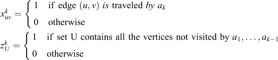
Here, we formulate the problem in such a way that we can apply the primal-dual technique. The decision variables used in the formulation are defined as follows:

Decision variables

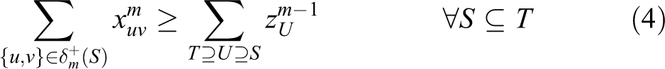
\begin{array}{l} x_{u v}^{k} = {\begin{array}{l} 1 & if edge (u, v) i s traveled b y a_{k} \\ 0 & otherwise \end{array} \\ z_{U}^{k} = {\begin{array}{l} 1 & if set U contains all the vertices not visited by a_{1}, \dots, a_{k - 1} \\ 0 & otherwise \end{array} \end{array}

First, let us consider the first robot, $a_{1}$ . Since we are going to relax some of the constraints at the end, only the entering edges are considered at this time. For any $S \supseteq T$ , at least one edge must be chosen from $δ_{1}^{+} (S)$ for the route of $a_{1}$ , if there is at least one vertex in S that is not connected to any other depots, that is, $\sum_{e \in δ_{1}^{+} (S)} x_{u v}^{1} \geq 1$ if $\sum_{T \supseteq U \supseteq S} z_{U}^{1} = 0$ , because $\sum_{T \supseteq U \supseteq S} z_{U}^{1} = 1$ only if U contains all the vertices assigned to $a_{1}$ . Thus, the requirement can be written as $\sum_{{u, v} \in δ_{1} (S)} x_{u v}^{1} \geq 1 - \sum_{T \supseteq U \supseteq S} z_{U}^{1}$ . Now, consider $a_{k}$ where $k = 2, \dots, m - 1$ . For any $S \supseteq T$ , an edge must be chosen from $δ_{k}^{+} (S)$ for the route of $a_{k}$ if at least one vertex in S is required to be visited by $a_{k}$ . This requirement can be expressed as $\sum_{{u, v} \in δ_{k} (S)} x_{u v}^{k} \geq \sum_{T \supseteq U \supseteq S} (z_{U}^{k - 1} - z_{U}^{k})$ for $k = 2, \dots, m - 1$ . Finally, for $a_{m}$ , $z_{U}^{m - 1} = 1$ , only if U contains all vertices that needs to be visited by $a_{m}$ . Thus, the constraint can be written as $\sum_{{u, v} \in δ_{m} (S)} x_{u v}^{m} \geq \sum_{T \supseteq U \supseteq S} z_{U}^{m - 1}$ . The constraints regarding payloads can be represented as $x_{i j}^{k} (q_{k} - r_{i}) \geq 0$ and $x_{i j}^{k} (q_{k} - r_{j}) \geq 0$ , for all $(i, j) \in E_{k}, k = 1, \dots, m$ . However, we already reflected the job handling restrictions by setting costs of unavailable jobs to the large constant M, the constraints are relaxed in the formulation. Furthermore, by relaxing integer constraints to be non-negative, we can formulate the linear program (LP) relaxation as follows

C_{L P} = min \sum_{k = 1}^{m} \sum_{{u, v} \in E_{k}} c o s t_{u v}^{k} x_{u v}^{k}

subject to

\sum_{{u, v} \in δ_{1}^{+} (S)} x_{u v}^{1} \geq 1 - \sum_{T \supseteq U \supseteq S} z_{U}^{1} \forall S \subseteq T

\begin{array}{l} \sum_{{u, v} \in δ_{k}^{+} (S)} x_{u v}^{k} \geq \sum_{T \supseteq U \supseteq S} (z_{U}^{k - 1} - z_{U}^{k}) \\ \forall S \subseteq T; k = 2, \dots, m - 1 \end{array}

\sum_{{u, v} \in δ_{m}^{+} (S)} x_{u v}^{m} \geq \sum_{T \supseteq U \supseteq S} z_{U}^{m - 1} \forall S \subseteq T

x_{u v}^{k} \geq 0 \forall {u, v} \in E_{k}, k = 1, \dots, m

z_{U}^{k} \geq 0 \forall U \subseteq T, k = 1, \dots, m - 1

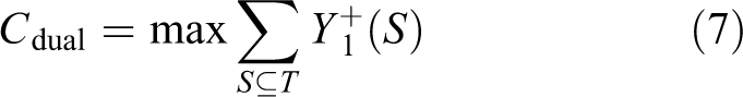
By introducing the dual variables $Y_{k}^{+} (S)$ for the constraints of equations (2) to (4), a dual problem of LP in equations (1) to (6) can be induced as shown below.

C_{dual} = max \sum_{S \subseteq T} Y_{1}^{+} (S)

subject to

\begin{array}{l} \sum_{S : (u, v) \in δ_{k}^{+} (S)} Y_{k}^{+} (S) \leq c o s t_{u v}^{k} \\ \forall {u, v} \in E_{k}, k = 1, \dots, m \end{array}

\begin{array}{l} \sum_{S \subseteq U} Y_{k}^{+} (S) \leq \sum_{S \subseteq U} Y_{k + 1}^{+} (S) \\ \forall U \subseteq T, k = 1, \dots, m - 1 \end{array}

Y_{k}^{+} (S) \geq 0 \forall S \subseteq T, k = 1, \dots, m

We use this dual problem to find a heterogeneous directed spanning forest (HDSF), which is a collection of m trees with each tree spanning a subset of targets from each depot. We then use the result for dispatching. In the algorithm, each dual variable $Y_{k}^{+} (S)$ is treated as the cost that each set S is willing to pay to be reached from $i_{k}$ . The details would be discussed in the following section.

A primal-dual heuristic for finding a HDSF

In this section, we propose a primal-dual heuristic to find an HDSF. The main concept of the algorithm is very simple. In the algorithm, each dual variable implies the cost each set needs to pay to be visited by one of the robots. Initially, all dual variables are set to zero. In every iteration, the algorithm look for the dual variable(s) that can be increased, without violating any of the dual constraints in equations (8) to (10), with the minimum value. The edge(s) that made one of (8) tight is(are) added to the corresponding tree(s). By repeating iterations, we can find a forest that makes every vertex reachable from at least one of the depots and thus complete the HDSF by removing unnecessary edges. Since we set the travel cost for the jobs that cannot be taken to the very large constant M, the algorithm will avoid choosing those edges and instead choose the edges with low costs.

The pseudocode of the algorithm based on the primal-dual technique is presented with three steps in Algorithm 1 to 3. In Figures 2 to 5, every step of the algorithm for an instance with two robots and five jobs is presented. In the algorithm, a component is active if it does not have any entering edges or is not reachable from any of the depots. A component is inactive if it has at least one entering edge or is reachable from one of the depots. A component is called $v i o l a t e d$ when the component does not have any entering edges.

Algorithm 1

Initialization step of the primal-dual heuristic.

Algorithm 2

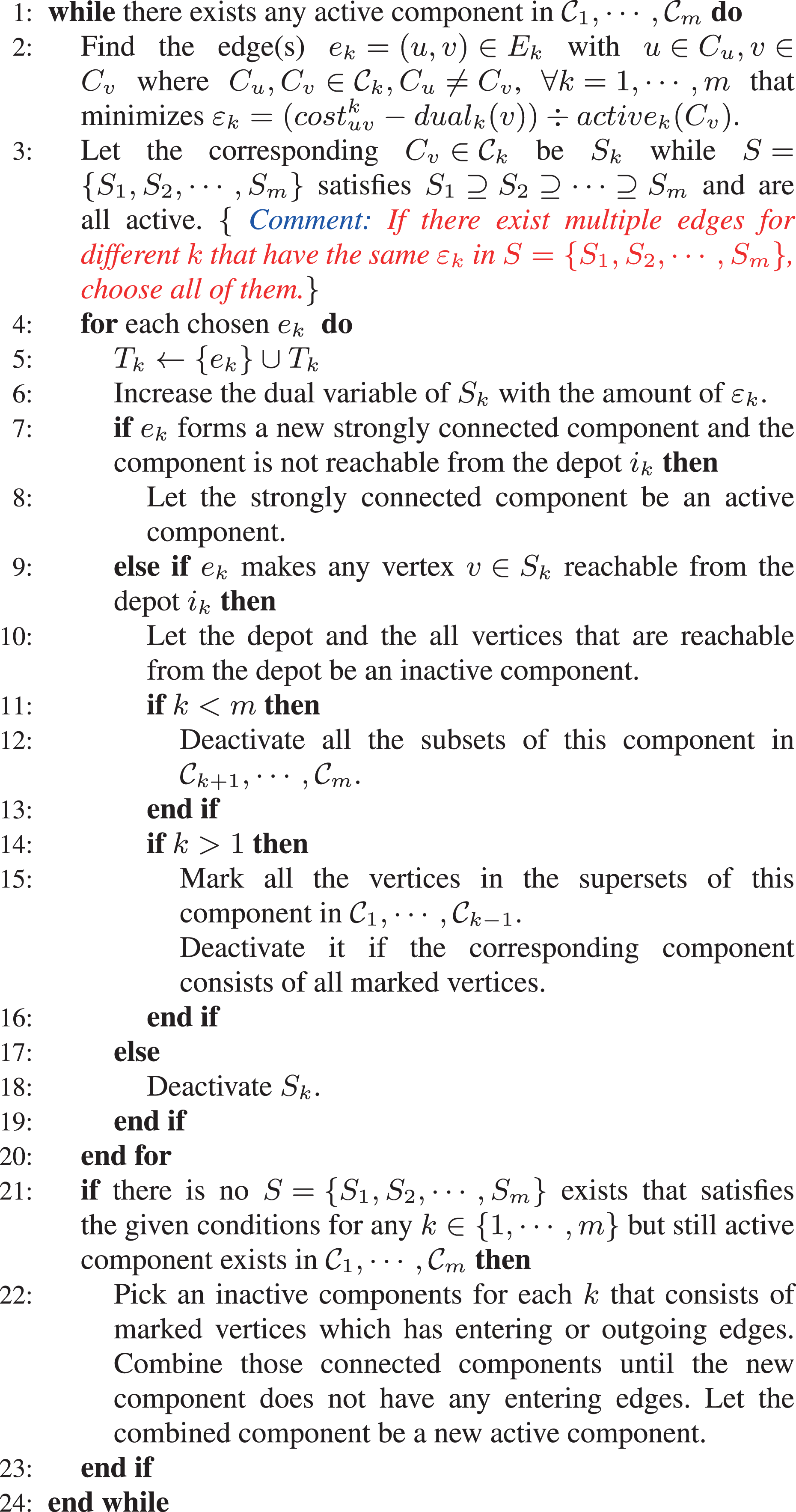
Main loop of the primal-dual heuristic.

Algorithm 3.

Pruning step of the primal-dual heuristic.

Figure 2.

Initial status of an instance with two robots and five jobs. The blue filled circles represent an active status, and the grey filled circles represent an inactive status. At initialization, each vertex is in its distinct connected component (line 2 in Algorithm 1), and all jobs are active while all depots are inactive (line 5–6 in Algorithm 1). In this instance, the payloads of robots are given as $Q = {5, 4}$ , while the required payloads of jobs are given as $R = {3, 1, 2, 5, 1}$ . Thus, $r_{2}$ cannot take $j_{4}$ in this instance.

Figure 3.

The iteration 1 to 4 of the main loop of an instance with two robots and five jobs. The red edges represent those added at the corresponding iteration. The line number in parenthesis indicates the line in Algorithm 2 that is related to the action in each iteration. (a) Iteration#1. The edge of i ₂ to j ₃ is added to T₂. Because {j ₃} ϵ C ₂ became reachable from i ₂ (line 9), {i ₂; j ₃} has become an inactive component. (line 10) The superset {j ₃} ϵ C ₁ has been marked and deactivated (line 15). (b) Iteration#2. The edges of j ₅ to j ₁ have been added to both trees. {j ₁} ϵ C ₁ and {j ₁} ϵ C ₂ are deactivated (line 18). (c) Iteration#3. The edge of j ₃ to j ₄ is added to T ₁. {j ₄} ϵ C ₁ is deactivated (line 18). (d) Iteration#4. The edges of j ₁ to j ₅ are added to both trees. By adding the edges, new strongly connected components are formed (line 7) and {j ₁; j ₅} in both C ₁; C ₂ became new active components at the end of the iteration (line 8).

Figure 4.

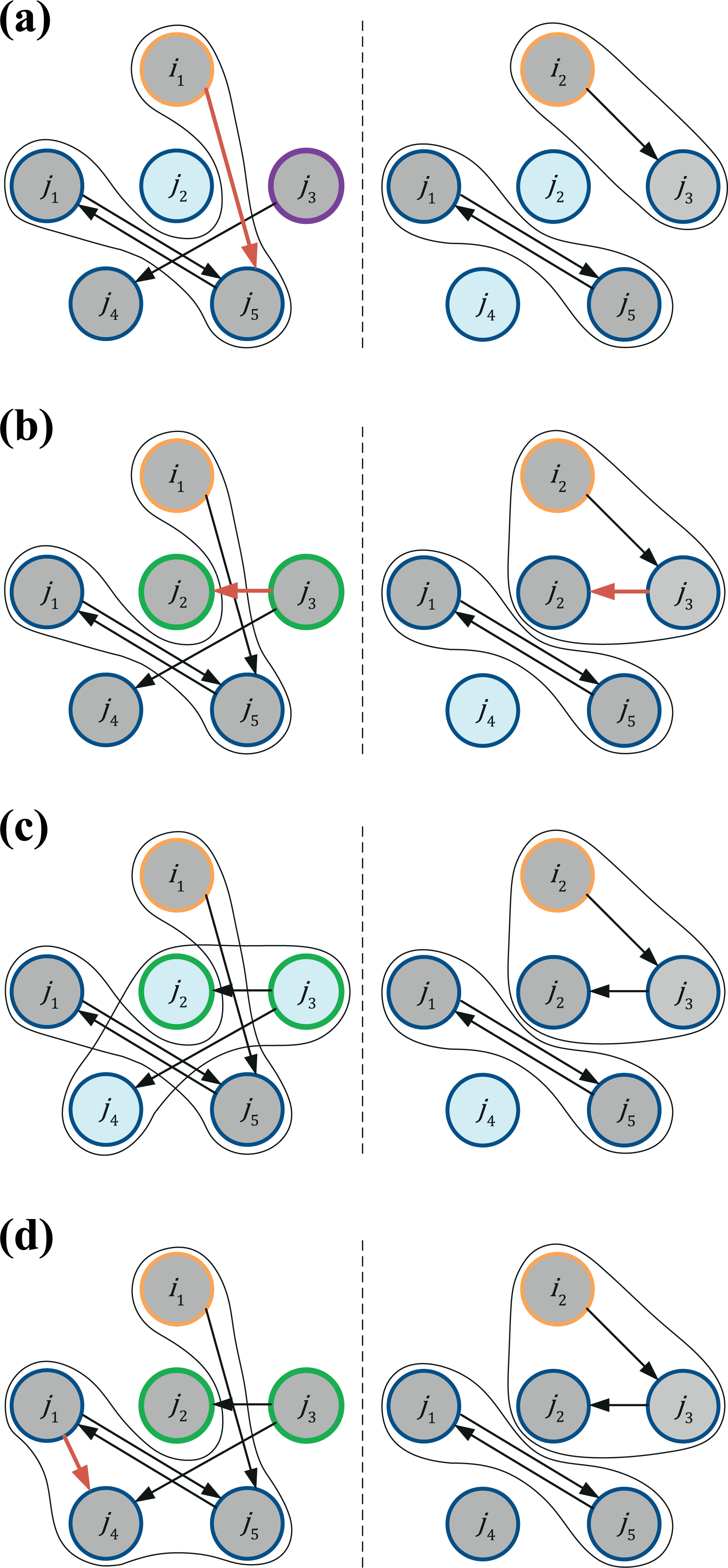
The iteration 5 to 7 of the main loop of an instance with two robots and five jobs, continued from Figure 3. (a) Iteration#5. The edge of i ₁ to j ₅ is added to T ₁. Because {j ₁; j ₅} ϵ C ₁ has become reachable from i ₁ (line 9), {i ₁; j ₁; j ₅} has become a new inactive component in C ₁ (line 10). The subset {j ₁; j ₅} ϵ C ₂ is deactivated (line 12). (b) Iteration#6. The edges of j ₃ to j ₂ are added to both trees. Now, {j ₂} ϵ C ₂ has become reachable from i ₂ (line 9) and {i ₂; j ₂; j ₃} ϵ C ₂ has become a new inactive component (line 10). The supersets {j ₂}, {j3} ϵ C ₁ are marked and deactivated (line 15). (c) Iteration#6-1. Since there is no active component without any entering edge in C ₁ (line 21), the set {j ₃} has been picked and combined with the sets {j ₂} and {j ₄} that are connected with outgoing edges from {j ₃}. Since {j ₂; j ₃; j ₄} does not have any entering edges, it becomes a new active component in C ₁ (line 22). (d) Iteration#7. The edge of j ₁ to j ₄ is added to T ₁. {j ₄} has become reachable from i ₁ (line 9) and {i ₁; j ₁; j ₄; j ₅} has become a new inactive component in C ₁ (line 10). The subset {j ₄} ϵ C ₂ is deactivated (line 12). Since all components are inactive, the main loop is terminated at this iteration (line 1).

Figure 5.

The generated HDSF after pruning step of an instance with two robots and five jobs. During pruning step, all the unnecessary edges $((j_{2}, j_{3}) \in E_{1}; (j_{1}, j_{5}) \in E_{1}, E_{2}; (j_{3}, j_{4}) \in E_{1}; (j_{5}, j_{1}) \in E_{2} in sequence)$ were removed, as presented in line 2–6 in Algorithm 3. HDSF: heterogenous directed spanning forest.

The initialization step is presented in Algorithm 1. At initialization, for all $k \in {1, \dots, m}$ , $T_{k}$ is empty and each $C_{k}$ consists of components where each vertex is in its distinct connected component. All components containing jobs are active and all components containing depots are inactive. For every $k \in {1, \dots, m}$ , each vertex in $v \in V_{k}$ is initially unmarked and all dual variables are set to zero. The initialized status of an instance with two robots and five jobs is shown in Figure 2.

The main loop of the heuristic is presented in Algorithm 2. During each iteration of the main loop, we find an active violated component in all $C_{k}$ which has the dual variable that can be increased, without violating any of the constraints in equation (8), with the minimum value. Let the corresponding component be $S_{k}$ for $a_{k}$ , and we choose one of its active subsets or supersets from each $C_{t}$ for all $t = 1, \dots, m$ , such that $S_{1} \supseteq S_{2} \supseteq \dots \supseteq S_{m}$ . If there exist multiple edges that can be added by increasing the dual variables with the same amount in the chosen ${S_{1}, \dots, S_{m}}$ , choose all of them. For each k that has been chosen, let the corresponding entering edge be denoted by $e_{k} \in E_{k}$ and add this new edge to its corresponding tree $T_{k}$ . Three possible cases could arise by adding $e_{k}$ . First, a new strongly connected component is generated, but it is still not reachable from the depot $i_{k}$ . In this case, the new strongly connected component now becomes a new active component. Second, at least one vertex, which was active at the beginning of the iteration, becomes reachable from the depot $i_{k}$ . In this case, let the depot and all the vertices that are reachable from the depot be an inactive component. If $k < m$ , deactivate all the subsets of this component in $C_{k + 1}, \dots, C_{m}$ . If $k > 1$ , mark all the vertices in the supersets of this component in $C_{1}, \dots, C_{k - 1}$ and deactivate if the corresponding component only consists of marked vertices. This marking process is included to ensure that the constraints in equation (9) are not violated at any time. Lastly, if neither the first nor second case happens, deactivate $S_{k}$ .

If there is no active component without any entering edge in $C_{k}$ for any $k \in {1, \dots, m - 1}$ but the main loop cannot be terminated, the algorithm forces it to make active components for those $C_{k}$ by combining inactive connected components. By the way we built the algorithm, there must be at least one component which contains unmarked vertices that can be combined with a component that has marked vertices. Those components now become a new active violated component in $C_{k}$ . During implementation, we picked an inactive component in a corresponding $C_{k}$ that consists of marked vertices which has entering or outgoing edges and combined it with connected components until the new component does not have any entering edges. When all the components are inactive, the main loop terminates. The details of main loop of each iteration with an instance have been presented in Figures 3 and 4.

As the final step of the algorithm, we perform reverse deleting in pruning step to obtain the final forest as shown in Algorithm 3. Let $e_{x}$ be the edge that is added to F at x th iteration of the main loop. In reverse order (from the total number of the iterations of the main loop down to 1), if F is feasible without $e_{x}$ , then remove it from F. If multiple edges were added in the same iteration, consider the edge for $r_{k}$ with largest k in order. Otherwise, leave $e_{x}$ in F. Figure 5 shows the final HDSF of an instance after the pruning step. Finally, in Lemma 1, we prove the feasibility of the proposed algorithm and analyze the running time in Lemma 2.

Lemma 1

The proposed primal-dual heuristic (in Algorithms 1 to 3) produces a feasible HDSF. Each of the vertices is reachable from one of the depots and every vertex appears only once in the forest.

Proof

During the main loop, a component can be deactivated only if one of the following conditions is satisfied. (1) The edge added to the forest does not form any new strongly connected component, and none of the vertices in the component is reachable from one of the depots (this corresponds to line 18 in Algorithm 2). (2) The component has become reachable from its depot (this corresponds to line 10 in Algorithm 2). (3) One of its subsets or supersets becomes reachable from its depot (this corresponds to line 12 and 15 in Algorithm 2). The vertices would become reachable from one of the depots if (2) or (3) happens at least once at the time of termination.

Assume that only one active component is left for all $C_{k}$ after having case 1 for all iterations. Then there exist only two cases that can happen in the next iteration. Either the component becomes reachable from one of the depots and terminates the loop or a new active strongly connected component is formed and continues. This would be true until there exists only one large active component that contains all the vertices left except the depot, which implies the latter case cannot happen at the next iteration. Thus, at least one edge starting from one of the depots should be added before the termination. This implies that at the time of termination, each vertex is connected to at least one of the depots. Since we perform reverse deleting steps after the main loop, even if there existed vertices that were connected to multiple depots, the redundant edges would be removed and only one depot would be left at the end of the algorithm. Hence, the algorithm produces a feasible HDSF. □

Lemma 2

The proposed primal-dual heuristic runs in polynomial time.

Proof

In Algorithm 2, each time through the loop, we find the minimum edge(s) by extracting the minimum element from active components. Since there are at most n components for each robot at any point in time, each iteration will have $O (n)$ searches, yielding a time bound of $O (n log (n))$ per iteration, or $O (n^{2} log (n))$ for the entire loop. Algorithm 3 can be run in $O (n)$ time since there are $O (n)$ edges in F. Thus, the proposed heuristic can be run in $O (n^{2} log (n))$ , which is polynomial time. □

The resulted HDSF would be utilized as the partition of the vertices. The connected vertices in each tree become a job assignment for each robot. The routing process could be done by solving HPP within the assignment using existing algorithm. We applied Lin–Kernighan heuristic (LKH)¹⁷ to solve HPP in the implementation, which is discussed in the following section.

Computational results

The proposed algorithm is implemented and run for different sizes and instances. The simulation is performed in a virtual manufacturing system environment as shown in Figure 1. The number of robots varied from four to six, and the number of jobs varied from 20 to 40. We generated and tested 50 instances for each problem size. The locations (nodes) of depots, pickup, and delivery were generated with a uniform distribution from node#1 to node#60. The payloads of robots and the required payloads of jobs were generated from 1 to 5, also with a uniform distribution. All computational experiments were run on Intel Core i5-7600 CPU @3.5 GHz with 8 GB RAM. For each instance, the cost matrices of the robots were generated using improved A* algorithm. The cost function of traveling from node a to node b was set to travel time as $distance (a, b) / v_{m} + α \times c o s t_{R}$ , where $v_{m}$ is the average velocity of the robot and $c o s t_{R}$ is the time required to rotate the robot in right or left direction. Depending on the previous movement of the robot, α is set to 1, if and only if the robot needs any rotation to move to the next candidate node. The Euclidean distance from current node to node b was used as the heuristic function. The cost of jobs that each robot cannot take is set to a very large constant M. We set $M {= 10}^{6}$ in our simulation. Using the cost matrices, the proposed primal-dual heuristic was applied to obtain job assignments. For each partition, the path was generated using LKH, which is available online.¹⁸ Figure 6 shows the final routes of an instance with 4 robots and 10 jobs.

Figure 6.

The final routes for each robot of an instance of 4 robots and 10 jobs solved by the proposed heuristic. The payloads of each robot were $Q = {5, 4, 3, 2}$ , and the required payloads for each job were $R = {1,2,1,2,1,4,3,1,5,1}$ . This implies that $a_{1}$ can take all given jobs and $a_{2}$ can take all the jobs except $j_{9}$ . $a_{3}$ cannot take $j_{6}, j_{9}$ and $a_{4}$ cannot take $j_{6}, j_{7}, j_{9}$ . In each plot, the depot and the assigned jobs’ pickup and delivery nodes are presented. The results show that $a_{1}$ has completed $j_{6}, j_{9}, j_{4}, j_{7}$ in sequence, and $a_{2}$ completed $j_{2}, j_{8}, j_{5}$ in sequence. $a_{3}$ and $a_{4}$ accomplished $j_{1}, j_{3}$ , and $j_{10}$ , respectively. Thus, all assignments satisfy the payload restrictions.

To verify the performance and computation time of the proposed algorithm, we have also applied LP rounding method¹ on the multiple Asymmetric HPP and applied LKH for routing for the same instances. The LP rounding of the problem was solved by CPLEX.¹⁹ We compared the results produced by the algorithms. To compare solution qualities, a posteriori bound is calculated by $\frac{c o s t_{a l g o}^{I}}{c o s t_{L P}^{I}}$ for every instance I, where $c o s t_{a l g o}^{I}$ represents the cost produced using algo algorithm for instance I, and $c o s t_{L P}^{I}$ represents the cost produced by solving LP relaxation of the problem, which is one of the well-known lower bound of the problem, for instance I. The average and maximum a posteriori bounds are presented in Figure 7. In Figure 7, we can see that a posteriori bound of the primal-dual heuristic does not vary depending on the problem size, and the produced solution qualities are relatively consistent. The maximum a posteriori bounds stayed slightly above of LP rounding method but did not show any considerable difference.

Figure 7.

The average (the left column) and the maximum (the right column) a posteriori bounds.

The average and maximum computation times of the instances are shown in Tables 1 and 2, respectively. As we can see from the results, the proposed heuristic solves the problem in a relatively short period even for the largest problem size. Because the LP rounding method is based on LP relaxation, which is very time-sensitive method, the computation time increased significantly as the problem size increased. Even for the largest problem sizes, the maximum computation time of the primal-dual heuristic was only about 8 s, while that of the LP rounding was over 23,830 s (more than 6 h). These results indicate that the proposed heuristic is promising, considering the complexity of the problem, especially when the problem sizes are huge.

Table 1.

The average computation times in seconds.

Four robots
No. of jobs	LP rounding + LKH	Primal-dual heuristic
20	0.79	0.41
30	34.74	0.85
40	1474.37	1.62
Five robots
No. of jobs	LP rounding + LKH	Primal-dual heuristic
20	1.05	0.79
30	67.68	4.58
40	2237.90	8.62
Six robots
No. of jobs	LP rounding + LKH	Primal-dual heuristic
20	1.39	0.79
30	158.95	1.93
40	4546.33	3.86

LKH: Lin–Kernighan heuristic; LP: linear program.

Table 2.

The maximum computation times in seconds.

Four robots
No. of jobs	LP rounding + LKH	Primal-dual heuristic
20	0.79	0.97
30	162.92	1.18
40	34416.4	2.11
Five robots
No. of jobs	LP rounding + LKH	Primal-dual heuristic
20	6.19	3.46
30	628.11	7.04
40	11752.7	11.10
Six robots
No. of jobs	LP rounding + LKH	Primal-dual heuristic
20	5.52	1.71
30	1547.95	2.85
40	23830.3	7.87

LKH: Lin–Kernighan heuristic; LP: linear program.

Conclusion

The study addressed the path planning problem for a system with multiple transportation robots having different loading conditions. By reflecting payload restrictions and job handling costs in the travel costs, the problem could be represented as a multiple depot heterogeneous asymmetric HPP. A heuristic based on the primal-dual technique is proposed to solve the problem. From the implementation results, the effectiveness of the proposed algorithm has been demonstrated. We hope to improve the algorithm further to include an approximation ratio. We also believe this to be a good first step toward developing an algorithm that would minimize the last job finishing time, as the objective becomes a min-max problem, while considering both structural and functional heterogeneity simultaneously.

Footnotes

Declaration of conflicting interests

The author(s) declared no potential conflicts of interest with respect to the research, authorship, and/or publication of this article.

Funding

The author(s) disclosed receipt of following financial support for the research, authorship, and/or publication of this article: This research was supported by the NRF, MSIP (Grant No. NRF-2017R1A2A1 A17069329) and by the Agriculture, Food and Rural Affairs Research Center Support Program (Grant No. 714002-07), MAFRA, Korea.

ORCID iD

Jungyun Bae

References

Bae

. Algorithms for multiple vehicle routing problems. PhD dissertation, Texas A&M University, College Station, TX, USA, 2014.

Vazirani

. Approximation algorithms. Berlin: Springer, 2004.

Sundar

Rathinam

. A primal-dual heuristic for a heterogeneous unmanned vehicle path planning problem. Int J Adv Robotic Syst 2013; 10(10).

Yadlapalli

Bae

Rathinam

. Approximation algorithms for a heterogeneous multiple depot hamiltonian path problem. In: Proceedings of the 2011 American control conference, San Francisco, CA, USA, 29 June–1 July 2011, pp. 2789–2794, Washington DC: IEEE.

Tovey

Sharon

. Multi-agent path finding with payload transfers and the package-exchange robot-routing problem. In: Proceedings of 2016 AAAI conference on artificial intelligence. Phoenix, Arizona, 12–17 February 2016, pp. 3166–3173, ACM. DOI: 10.5772/56486.

Lagoudakis

Markakis

Kempe

. Auction-based multi-robot routing. In: Proceedings of the 2005 international conference on robotics: science and systems (ROBOTICS). Cambridge, Massachusetts, 8–11 June 2005, pp. 343–350. Cambridge, MA, USA: MITPress.

Choi

Brunet

How

. Consensus-based decentralized auctions for robust task allocation. IEEE Trans Robot 2009; 25(4): 912–926.

Schneider

Sklar

Parsons

Auction-based task allocation for multi-robot teams in dynamic environments. In: Dixon

Tuyls

(eds) TAROS 2015: towards autonomous robotic systems, Liverpool, UK, 18 July 2015, pp. 246–257. Cham: Springer International Publishing.

Rathinam

Sengupta

Darbha

. A resource allocation algorithm for multi-vehicle systems with non-holonomic constraints. IEEE Trans Auto Sci Eng 2007; 4(1): 98–104.

10.

Rathinam

Sengupta

. Lower and upper bounds for a multiple depot uav routing problem. In: IEEE control and decision conference. San Diego, California, USA, 13–15 December 2006.

11.

Oberlin

Rathinam

Darbha

. Today’s traveling salesman problem. IEEE Robot Auto Magazine 2010; 17(4): 70–77.

12.

Levy

Sundar

Rathinam

. Heuristics for routing heterogeneous unmanned vehicles with fuel constraints. Math Prob Eng 2014; 2014(3): 12.

13.

Frieze

Galbiati

Maffioli

. On the worst-case performance of some algorithms for the asymmetric traveling salesman problem. Networks 1982; 12(1): 23–39.

14.

Bae

Rathinam

. Approximation algorithm for a heterogeneous vehicle routing problem. Int J Adv Robotic Sys 2015; 12(8): 113.

15.

Rodrigues

. An extension of the christofides heuristic for the generalized multiple depot multiple traveling salesmen problem. Eur J Oper Res 2017; 257(3): 735–745.

16.

Hart

Nilsson

Raphael

. A formal basis for the heuristic determination of minimum cost paths. IEEE Tran Sys Sci Cybern 1968; 4(2): 100–107.

17.

Helsgaun

. An effective implementation of the Lin–Kernighan traveling salesman heuristic. Eur J Oper Res 2000; 126(1): 106–130.

18.

LKH-2.0.7 , 2009. http://www.akira.ruc.dk/keld/research/LKH/ (accessed 28 February 2019).

19.

IBM ILOG CPLEX Optimization Studio , 2017. https://www.ibm.com/us-en/marketplace/ibm-ilog-cplex (accessed 28 February 2019).

Efficient path planning for multiple transportation robots under various loading conditions

Abstract

Keywords

Introduction

Problem statement

Parameters

Problem formulation

Decision variables

A primal-dual heuristic for finding a HDSF

Lemma 1

Proof

Lemma 2

Proof

Computational results

Conclusion

Footnotes

Declaration of conflicting interests

Funding

ORCID iD

References