Sage Journals: Discover world-class research

Abstract

It is necessary for a mobile robot or even a multi-robot team to be able to efficiently plan a path from its starting or current location to a desired goal location. This is a trivial task when the environment is static. However, the operational environment of the robot is rarely static, and it often has many moving obstacles. The robot may encounter one, or many, of these unknown and unpredictable moving obstacles. The robot will need to decide how to proceed when one of these obstacles is obstructing its path. In this article, a new method of dynamic replanning is proposed to allow the robot to efficiently plan a path in such complex environments. Our proposed replanning method is based on an extended rapidly exploring random tree. The robot will modify its current plan when unknown random moving obstacles obstruct the path. We extend the proposed replanning method to multi-robot scenarios in which the ability to share path planning and search tree information is valuable. An efficient method of node sharing is proposed to allow the multi-robot team to quickly develop path plans. Various experimental results in both single and multi-robot scenarios show the effectiveness of the proposed methods.

Keywords

Mobile robots multi-robot path planning RRT RRT*

Introduction

Path planning has been one of the most researched problems in the area of robotics. The primary goal of any path planning algorithm is to provide a collision-free path from a start state to an end state within the configuration space of the robot. Probabilistic planning algorithms, such as the probabilistic roadmap method¹ and the rapidly exploring random tree (RRT),² provide a quick solution at the expense of optimality. Since its introduction, the RRT algorithm has been one of the most popular probabilistic planning algorithms. The RRT is a fast, simple algorithm that incrementally generates a tree in the configuration space until the goal is found.

The RRT has a significant limitation in finding an asymptotically optimal path and has been shown to never converge to an asymptotically optimal solution.^3,4 There is extensive research on the subject of improving the performance of the RRT. Simple improvements such as the bi-directional RRT and the rapidly exploring random forest improve the search coverage and speed at which a single-query solution is found. The anytime RRT⁵ provides a significant improvement in cost-based planning. Additionally, the extended RRT called RRT* algorithm^3,6 provides a significant improvement in the optimality of the RRT and has been shown to provide an asymptotically suboptimal solution.

Since the introduction of the RRT* algorithm, research has expanded to discover new ways to improve upon the algorithm. Research includes adding heuristics^7,8 or bounds⁹ to the algorithm in order to maintain the convergence of the algorithm but reduce the execution time. Additional research attempts to guide the algorithm through intelligent sampling¹⁰ or guided sampling through an artificial potential field.¹¹

In many scenarios, the operational environment is rarely static.^12

–15 The path from a single query will often be obstructed during execution. For that reason, the topic of replanning is very important to robotic path planning. It is not feasible to discard an entire search tree and start over.¹⁶ One method is to store waypoints and regrow trees called the execution extended RRT (ERRT).¹⁷ Another method (dynamic RRT [DRRT]) is to place the root of the tree at the goal location, so that only a small number of branches may be lost or invalidated when replanning.¹⁸ A combination of both ERRT and DRRT called multipartite RRT¹⁹ can maintain a set of subtrees that may be pruned and reconnected, along with previous states to guide regrowth. More recently, the RRT^X algorithm²⁰ has been incorporated into replanning. RRT^X is an algorithm that uses RRT* to continuously update the path during execution. The RRT^X is able to compensate for instantaneous changes in the static environment which is outside the scope of this work. Overall, there is little work considering robot replanning in complex environments where moving obstacles may obstruct the path.

Research on multi-robot teams has increased in recent years. These multi-robot teams are accomplishing tasks from cooperative sensing,^21,22 formation control,^23

–27 and target tracking and observation.²⁸ In a multi-robot scenario, it may be important for each robot on the team to quickly develop a path plan. If path plans are found quickly, then more time may be spent executing tasks, rather than planning to execute tasks.

The motivation of this work is to study robotic path planning in a complex two-dimensional (2-D) environment with unknown random obstacles. This environment is intended to be similar to real-world scenarios. A static or predictable environment is not representative to the real world. Often, the real world is unpredictable and full of randomly moving obstacles. A robot moving within the real world will need to be able to quickly develop a plan and modify that plan to avoid colliding with the obstacles. Ideally, the plan to avoid obstacles would maintain the optimality of a single-query path plan. Often, more than one robot will be moving throughout the environment. This work also studies a scenario where multiple robots share path planning information.

The major contribution of this work contains two parts. The first part is a new development of replanning algorithm based on RRT* for a mobile robot navigation in a dynamic environment with random, unpredictable moving obstacles. The second part is a novel development of RRT*-based path planning algorithm for multiple robots to share information about the environment to efficiently develop a path plan for each robot in the team. Various experimental results in both single and multi-robot scenarios are conducted to show the effectiveness of the proposed methods.

RRT and RRT*-based robot path planning

This section provides some background of the RRT and RTT* path planning methods. The comparison of these two methods associated with simulation results is provided.

The RRT* algorithm³ provides a significant improvement in the quality of the paths discovered in the configuration space over its predecessor the RRT.² The quality of the path is determined by the cost associated with moving from the start location to the end location. While RRT* does produce higher quality paths, the algorithm does have a longer execution time. The longer execution time of RRT* is due to the algorithm making many additional calls to the local planner in order to continuously improve the discovered paths.^3,16 RRT* operates in a very similar way as RRT. The algorithm builds a tree using random samples from the configuration space of the robot and connects new samples to the tree as they are discovered. RRT* has two primary differences comparing to RRT. The first difference is in the method that new edges are added to the tree. The second difference is an added step to change the tree in order to reduce path cost using the newly added vertex. Each of these differences contributes to the improvement of discovered paths over time and is reason RRT* will converge to an asymptotically suboptimal solution.

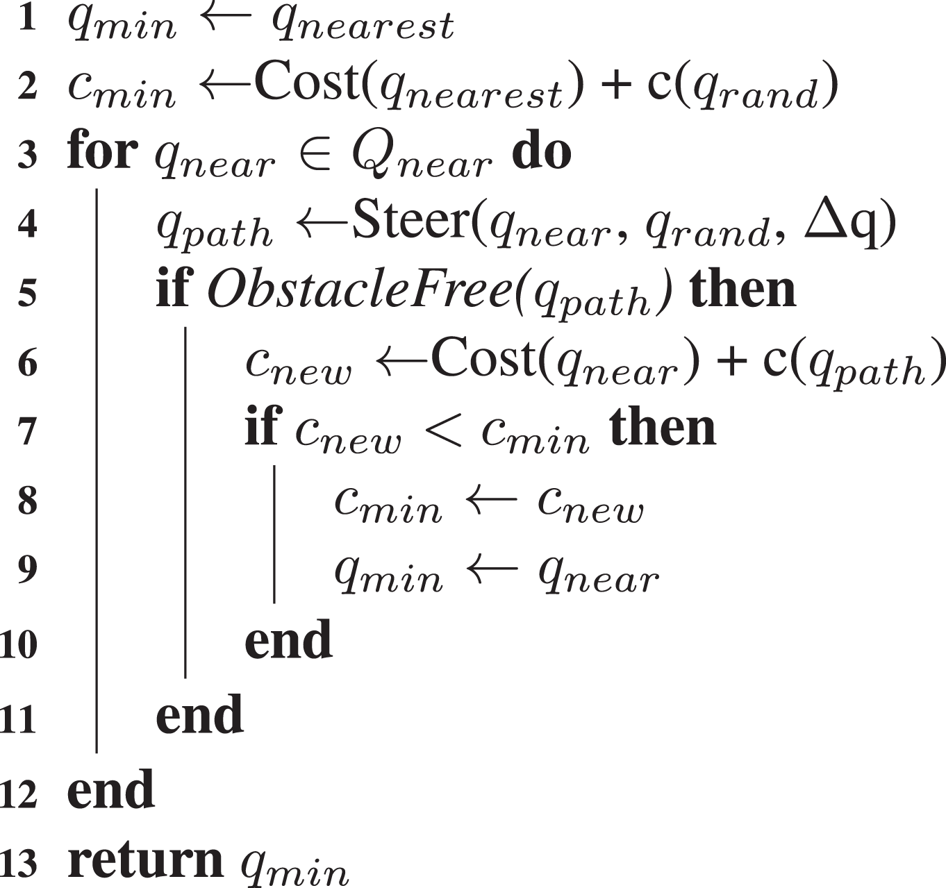
When a random vertex is added to the tree, the RRT will select the nearest neighbor as the parent for this new vertex and edge. RRT* will select the best neighbor as the parent for the new vertex. While finding the nearest neighbor, RRT* considers all the nodes within a neighborhood of the random sample. RRT* will then examine the cost associated with connecting to each of these nodes. The node yielding the lowest cost to reach the random sample will be selected as the parent, and the vertex and edge are added accordingly.

The RRT* algorithm begins in the same way as the RRT. However, when selecting the nearest neighbor, the algorithm also selects the set of nodes, $Q_{near}$ , in the tree that are in the neighborhood of the random sample $q_{rand}$ . Line 6 of algorithm 1 is the first major difference between the RRT* and the RRT. Instead of selecting the nearest neighbor to the random sample, the $C h o o s e P a r e n t ()$ function will select the best parent from the neighborhood of nodes.

Algorithm 1

$T = (V, E) \leftarrow$ RRT*( $q_{init}$ ).

Algorithm 2 describes the $C h o o s e P a r e n t ()$ function. This function maintains the node with the lowest total cost for reaching $q_{rand}$ . At line 1 of algorithm 2, the nearest neighbor, $q_{nearest}$ , is considered the minimum cost neighbor, or $q_{min}$ . At line 2, the cost associated with reaching the new random sample $q_{rand}$ using $q_{nearest}$ as the parent is stored as the current best cost, or $c_{min}$ . The algorithm then searches the set of nodes in the neighborhood of $q_{rand}$ . The $S t e e r ()$ function on line 4 of algorithm 2 will return a path from the nearby node, $q_{near}$ to $q_{rand}$ . If this path is obstacle free and has a lower cost than the current minimum cost, then the nearby node becomes the best neighbor, $q_{min}$ ,and this cost becomes the best cost $c_{min}$ (lines 7–9 of algorithm 2). When all nearby nodes have been examined, the function returns the best neighbor. The new random node is inserted into the tree using $q_{min}$ as the parent. The next step is the second major difference between the RRT* and the RRT algorithms. Line 8 of algorithm 1 calls the $R e w i r e ()$ function.

Algorithm 2

$q_{min} \leftarrow$ ChooseParent $(q_{rand}, Q_{near}, q_{nearest}, Δ_{q})$ .

The $R e w i r e ()$ function, described in algorithm 3, changes the tree structure based on the newly inserted node $q_{rand}$ . This function again uses the nearby neighborhood of nodes, $Q_{near}$ , as candidates for rewiring. The $R e w i r e ()$ function uses the $S t e e r ()$ function to get the path; except this time, the path will start from the new node, $q_{rand}$ and go to the nearby node, $q_{near}$ . If this path is obstacle free and the total cost of this path is lower than the current cost to reach $q_{near}$ (line 3 of algorithm 3), then the new node $q_{rand}$ is a better parent than the current parent of $q_{near}$ . The tree is then rewired to remove the edge to the current parent of $q_{near}$ and add an edge to make $q_{rand}$ the parent of $q_{near}$ . This is done using the $R e C o n n e c t ()$ function on line 4 of algorithm 3.

Algorithm 3

T ← Rewire $(T, Q_{near}, q_{min}, q_{rand})$ .

The functions $C h o o s e P a r e n t ()$ and $R e w i r e ()$ change the structure of the search tree when compared to the RRT algorithm.²¹ The tree generated by the RRT has branches that move in all directions. The tree generated by the RRT* algorithm rarely has branches that move back in the direction of the parent. The $C h o o s e P a r e n t ()$ function ensures that edges are created and always moving away from the start location. The $R e w i r e ()$ function changes the internal structure of the tree to ensure internal vertices do not add unnecessary steps on any discovered path. The $C h o o s e P a r e n t ()$ and $R e w i r e ()$ functions guarantee that the paths discovered will be asymptotically suboptimal because these functions are always minimizing the costs to reach each node within the tree.

Comparison results

To show how the RRT* outperforms the RRT, we did some simulation tests. The environment for all of the experiments is a complex 2-D environment that will also serve as the configuration space for the robot. The environment is complex due to the number of obstacles. The environment also contains several narrow passages, which can be difficult for sampling-based planners to overcome. There are also several suboptimal paths where the algorithm may get stuck. For each experiment, the path cost is measured in Euclidean distance. The environment is also intended to mimic a potential real-world situation where there will be streets or sidewalks and open areas such as parks and plazas. Figure 1 shows the environment used. The green circle in the upper-left corner is the goal location and the blue circle near the bottom center is the start location. The RRT found the path length of 117.278 units, while RRT* found the shorter path length of 103.960 units.

Figure 1.

Results of RRT (left) and RRT* (right) with 5000 nodes. The blue line represents the best path found and the black line represents the first path found by the RRT. RRT: rapidly exploring random tree; RRT*: extended rapidly exploring random tree.

Statistical comparison results

To be sure, the optimal path numbers were consistent; both RRT and RRT* were run 100 times using a search tree size of 5000 nodes. During each run, the search trees will find many different paths and a best or optimal path. For each simulation run, the path costs are averaged and stored; similarly, the optimal path cost for each run is stored. Figure 2 shows the average path cost over the 100 simulation runs.

Figure 2.

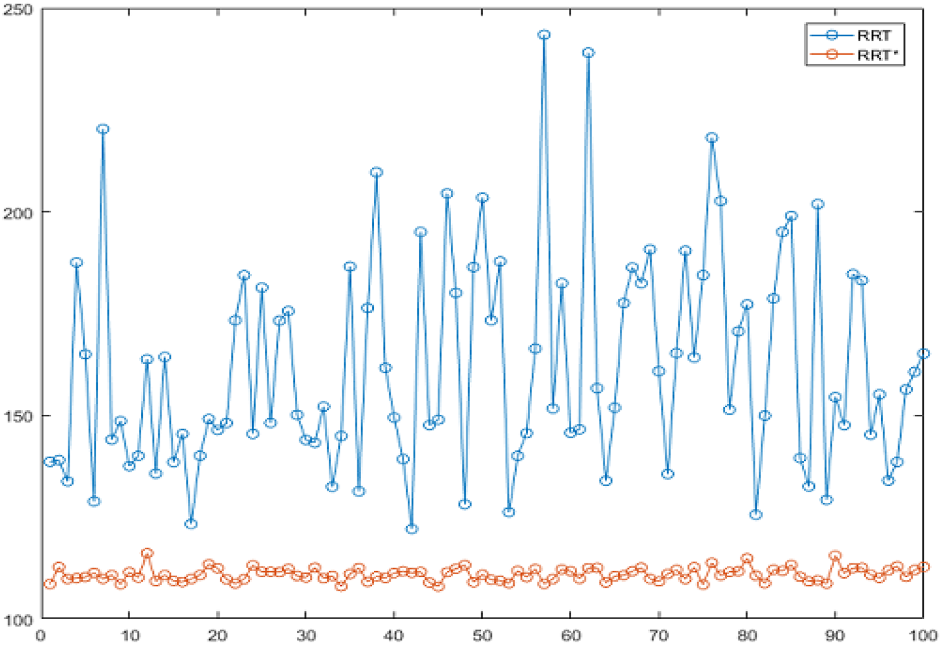
Average path cost for 100 RRT and RRT* simulations over the 100 simulation runs. RRT: rapidly exploring random tree; RRT*: extended rapidly exploring random tree.

The average path cost for the RRT* algorithm is very consistent, and the average path cost for the RRT is not. When examining the optimal path cost for each of the 100 simulations, shown in Figure 3, the average path cost is very similar. This is good for the RRT* algorithm, and it is not for the RRT algorithm. Figures 2 and 3 show how the RRT* algorithm will converge the discovered paths toward an optimal solution. Figures 2 and 3 also prove the randomness of the RRT. There is no convergence with the RRT paths. The average path cost is just as inconsistent as the cost of the best path.

Figure 3.

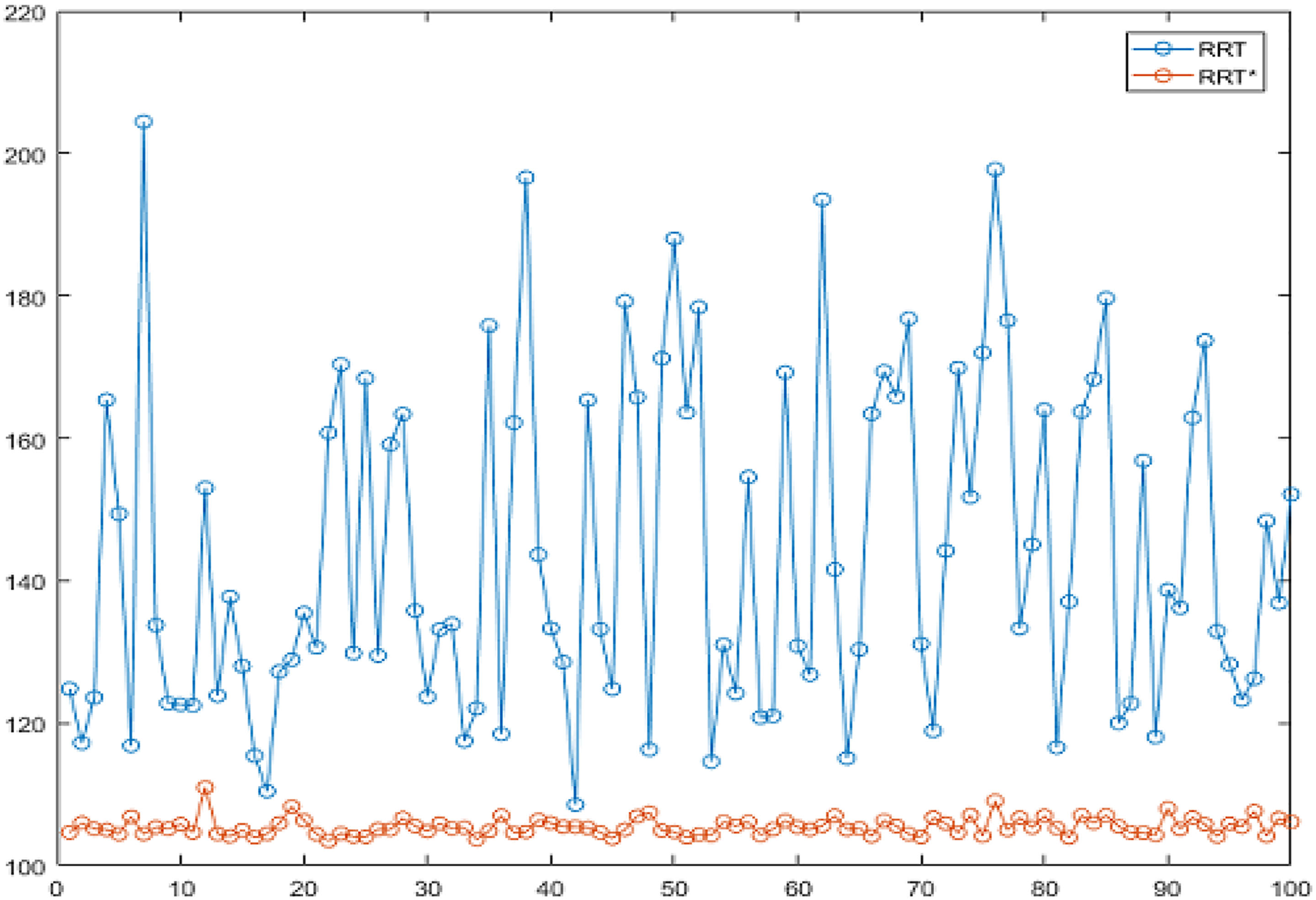
Optimal path cost for 100 RRT and RRT* simulations over the 100 simulation runs. RRT: rapidly exploring random tree; RRT*: extended rapidly exploring random tree.

The experiments conducted demonstrate how the RRT* algorithm will converge to an asymptotically suboptimal solution, whereas the RRT algorithm will not. The trade-off in reaching this asymptotically suboptimal solution is the number of nodes needed and the execution time to find the solution. Figure 4 shows the execution time required for each experiment. The blue line is the execution time of the RRT* algorithm and the red line is the execution time of the RRT algorithm. The execution time of RRT is nearly linear, when the number of nodes in the tree is doubled, the execution time is approximately doubled as well. The execution time of RRT* is exponential. The additional execution time comes from many extra calls to the local planner during the $C h o o s e P a r e n t ()$ and $R e w i r e ()$ functions. In the experiments above, there is very little improvement in the path when using 10,000 or 20,000 nodes. But, there is a significant increase in execution time. This is where the trade-off exists in the RRT* algorithm. The path can be improved, but the cost will be significant execution time and resources.

Figure 4.

Run times of each experiment of RRT versus RRT*. RRT: rapidly exploring random tree; RRT*: extended rapidly exploring random tree.

Dynamic replanning

Open problem

A real-world environment is not static, and it may be full of moving obstacles. These obstacles are often moving in unpredictable directions, which makes planning tasks to avoid them difficult. When a moving obstacle is known and follows a known trajectory, the configuration space can be modified to account for this trajectory. When the obstacle is unknown, the robot will need to be able to dynamically determine a course of action in order to avoid a collision. In this section, a method of dynamic replanning is proposed in order to avoid a random obstacle when it is detected by the robot.

Path execution

The robot is given a configuration space from which to build a tree using RRT* and determine the best path to reach the goal configuration from the start configuration. For the following simulations, the environment remains very similar. In all the experiments below, the robot can build a tree of varying sizes to evaluate the performance with different node densities. During the simulation, a few random moving obstacles are added to the environment, described in the next section. These obstacles represent a region of the configuration space that would be a collision if the robot was to enter.

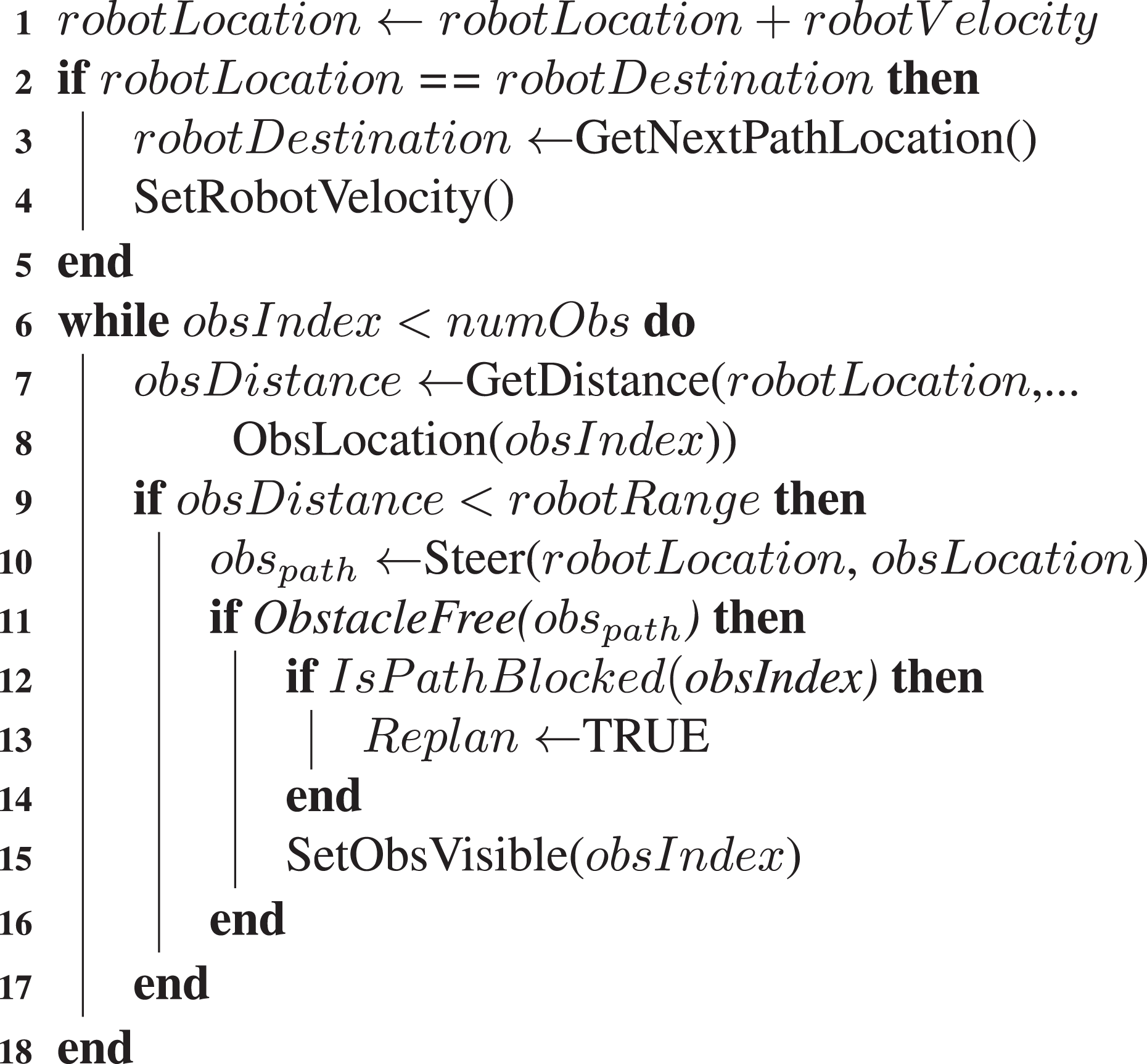
After the initial planning process, the robot begins to execute the optimal path found by the search tree. The robot traverses the optimal path by selecting the next node and required velocity vector to reach it (see lines 3 and 4 of algorithm 4). This process is described in algorithm 5 below. When the vertex is reached, the robot changes the velocity vector to move toward the next node. This process continues until the robot reaches the goal node. If the robot encounters a random moving obstacle that is obstructing the path, a replan event occurs.

Algorithm 4

ExecutePath().

Algorithm 5

UpdateRobotLocation().

Random moving obstacles and detection

The random moving obstacles force the robot to dynamically plan around the obstacle using RRT*. In order for the obstacles to move about the environment, a graph is created to provide the paths between the static obstacles, and the vertices are the intersections of these paths. Upon initialization of the simulation, the obstacles are placed at random vertices. The vertices are chosen such that the robot will have a chance to move before encountering a random obstacle. When the simulation begins, the moving obstacles choose a random adjacent vertex and begin moving toward that vertex (see lines 1 and 2 of algorithm 4). When the vertex is reached, a new random vertex is chosen and the obstacle moves in the new direction (see line 6 of algorithm 4).

Robots operating in a real-world scenario will have sensors, such as a light detection and ranging, to detect both static and dynamic obstacles. Sensors are not included in this simulation. Instead, a detection range is placed on the robot. The simulation controls whether or not a moving obstacle is within the detection range of the robot (see lines 7 and 8 of algorithm 5). If a moving obstacle is within range, the $S t e e r ()$ function is used to determine whether any static obstacles are blocking the robot’s line of sight to the moving obstacle.

The obstacle must be observed for a minimum of two time steps in order to determine the direction that the obstacle is moving. Once the direction is observed, the robot can determine whether the moving obstacle is blocking the path or not (see line 11 of algorithm 5). If the robot decides that the path is blocked, the replanning event begins.

Path replanning

Path replanning begins with the determination of whether or not the moving obstacle is blocking the path, described in the next section. Algorithm 6, below, lists all the steps executed during the replanning process. The next step is to find the location along the optimal path that is beyond the obstacle. Next, the tree generated by RRT* is modified and expanded in order to find a path around the obstacle. Finally, the best path around the obstacle is chosen and the execution of this subpath begins. Each of these steps is described in the following subsections.

Algorithm 6

T ← DoReplan().

Path obstruction

The method for determining whether the moving obstacle is blocking the path is a series of trigonometric functions using a direction vector from the robot to the moving obstacle and a comparison between the robot velocity vector and the moving obstacle velocity vector. Since the configuration space is 2-D, the inverse tangent can be used to find the angles of the vectors. To obtain the direction vector to the moving obstacle, use the below equation

{angle}_{direction} = a t a n 2 ((Y_{obs} - Y_{robot}), (X_{obs} - X_{robot}))

where $(X_{robot}, Y_{robot})$ is the position of the robot and $(X_{obs}, Y_{obs})$ is the position of the obstacle. This will return an angle in degrees over the range $(- 180, 180)$ . Similarly, the angle of the robot’s velocity vector can be obtained using the following equation

{angle}_{V_{robot}} = a tan 2 (V_{j}, V_{i})

where V_i and V_j are the X and Y components of the robot velocity vector, respectively. Using the angles from equations (1) and (2), the difference can be taken to see whether they are similar. If the absolute value of the difference between the two angles is less than some threshold, then the robot is moving toward the moving obstacle. Note, the angle difference is normalized to be in the range $(- 180, 180)$ before the absolute value is taken. This is done for all angle comparisons

| {angle}_{direction} - {angle}_{V_{robot}} | < {angle}_{thresh}

If the robot is moving in the direction of the random obstacle, the velocity vectors are examined. Substituting the obstacle velocity into equation (2) above, the angle of the obstacle velocity can be obtained. Next, the differences between the velocity vectors are found

{angle}_{V_{diff}} = | {angle}_{V_{robot}} - {angle}_{V_{obs}} |

There are three possibilities from this point. If the angle difference between the velocity vectors is less than the angle threshold, then the robot and the obstacle are moving in a similar direction. Second, if the angle difference between the velocity vectors is greater than $180 - {angle}_{thresh}$ , then the robot and the obstacle are approximately moving toward each other. Last, if the angle difference falls outside of these ranges, the moving obstacle and the robot are moving in different directions.

For the first case, the robot will simply follow the obstacle, until the obstacle changes direction, or the path takes the robot away from the obstacle. The robot will then choose from one of the other conditions. For the second case, the robot quickly activates a replan event to get out of the way. The random obstacle may move out of the way on its own, but there is no way of predicting that will occur. Finally, if the robot and the obstacle are moving in different directions, the robot ignores the obstacle unless it gets too close. This third condition catches the event that the robot moves out from a corner, and a random obstacle is detected very close by. This event is best summed up with the following example: when two people approach a hallway intersection, they will run into each other if they continue on their current course; it is only when they see each other that they can adjust to avoid a collision.

Establish replanning goal location

The second step in the replan event, line 2 of algorithm 6, is to find a location that will navigate the robot around the random obstacle. First, any nodes that are in collision with a random moving obstacle are invalidated, not deleted. The only exception is the goal location of the optimal path. After this step, an assumption had to be made to simplify and speed up the rest of the replanning process. The assumption is that the robot is currently following the best path in order to reach the goal location and should return to this path after the moving obstacle is avoided. Using this assumption, only the nodes along the optimal path are examined. Nodes that are farther from the robot than the random obstacle are candidate nodes. The node on the optimal path that is immediately following the node that is closest to the obstacle, without colliding, will be the replan goal location.

Modify search tree

The third step is to modify the original search tree in order to find a way around the moving obstacle. First, a node is added to the tree at the robot’s current location. Using the distance to the replan goal node as a metric, a sampling area is established (see line 3 of algorithm 6). Then, using $R e w i r e ()$ , every node within the sampling area is rewired such that the robot’s current location becomes the parent of that node. New nodes are then sampled within this area and added to the tree using RRT*. Since there are already many nodes in the tree, only a small number will need to be added. However, the number of nearest neighbors used during the $C h o o s e P a r e n t ()$ function and the $R e w i r e ()$ function is increased. This increase allows each new node to direct the existing tree toward the replan goal location.

Subpath selection and execution

When the search tree modification is complete, the best path to the replan goal location is found. Path execution will begin again as it did at the beginning of the simulation. When the robot reaches the replan goal location, the execution of the original optimal path resumes. If the robot encounters another moving obstacle and determines the path is obstructed again, the replanning is repeated. However, the replan goal location will always be a node on the original optimal path.

Results

The environment for all of the experiments is similar to the one described in section “RRT and RRT*-based robot path planning.” In the RRT* results presented below, the algorithm is set up with a maximum of 5000 nodes. The optimal path length is 98.48 units.

The RRT* evaluation was conducted in the following way: there is not a growth factor for extending the tree, and the tree is goal oriented. The expectation as the tree grows will be long branches. These branches are often inefficient; the RRT* $R e w i r e ()$ function will remove these long inefficient branches as the algorithm executes in favor of shorter, lower cost branches. The algorithm also has a maximum number of nearest neighbors or neighborhood size that is configurable to the algorithm. This implementation of RRT* has a maximum number of nearest neighbors equal to 1% of the total number of nodes.

Figure 6(c) shows the result of the search tree using the RRT* algorithm. The best path length found is 103.96 units.

Figure 5.

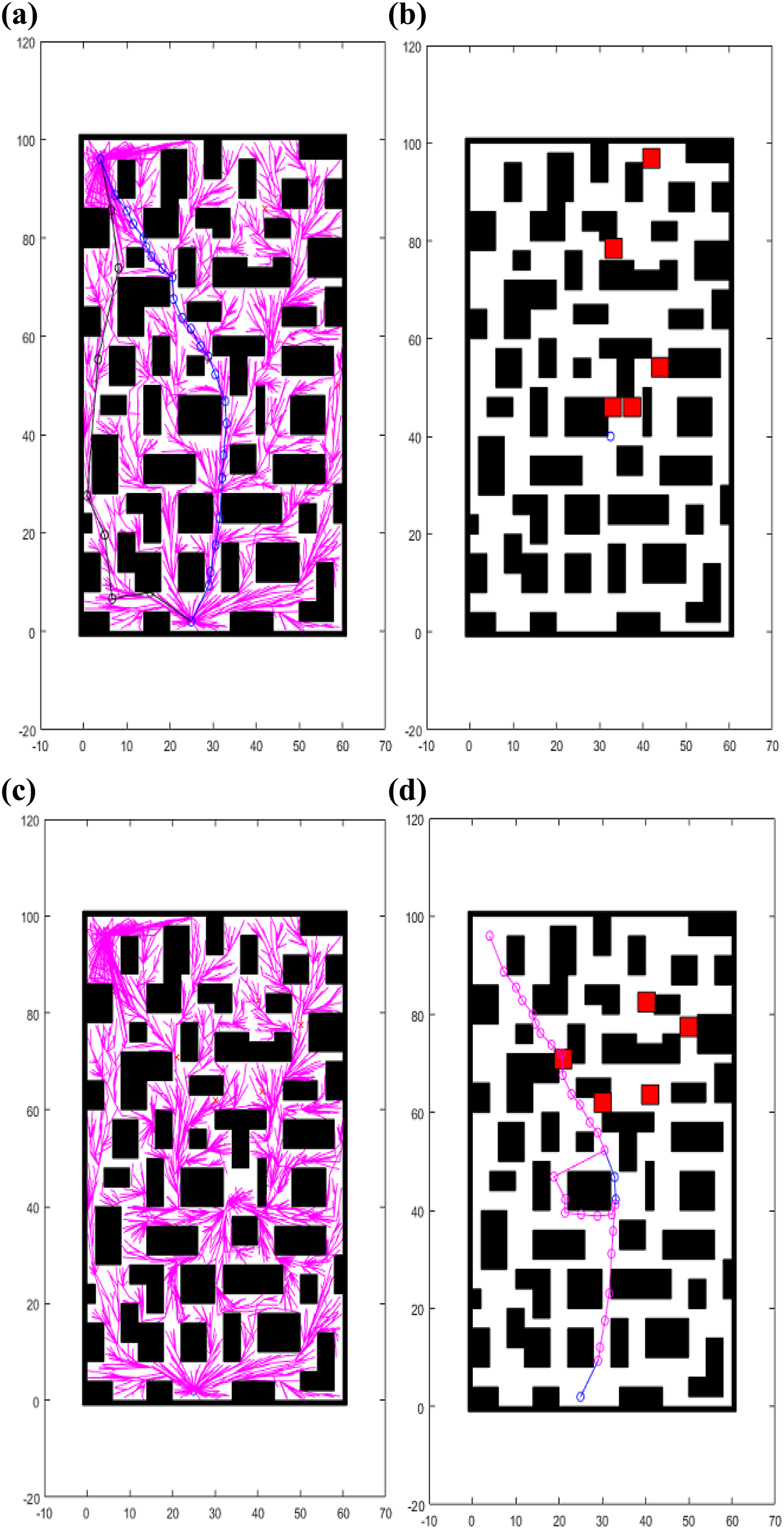
Replanning results from the first set. (a) Search tree and robot path. (b) Moving obstacles block the path. (c) Search tree after modification during replanning. (d) Final obstacle positions and the executed path.

Figure 6.

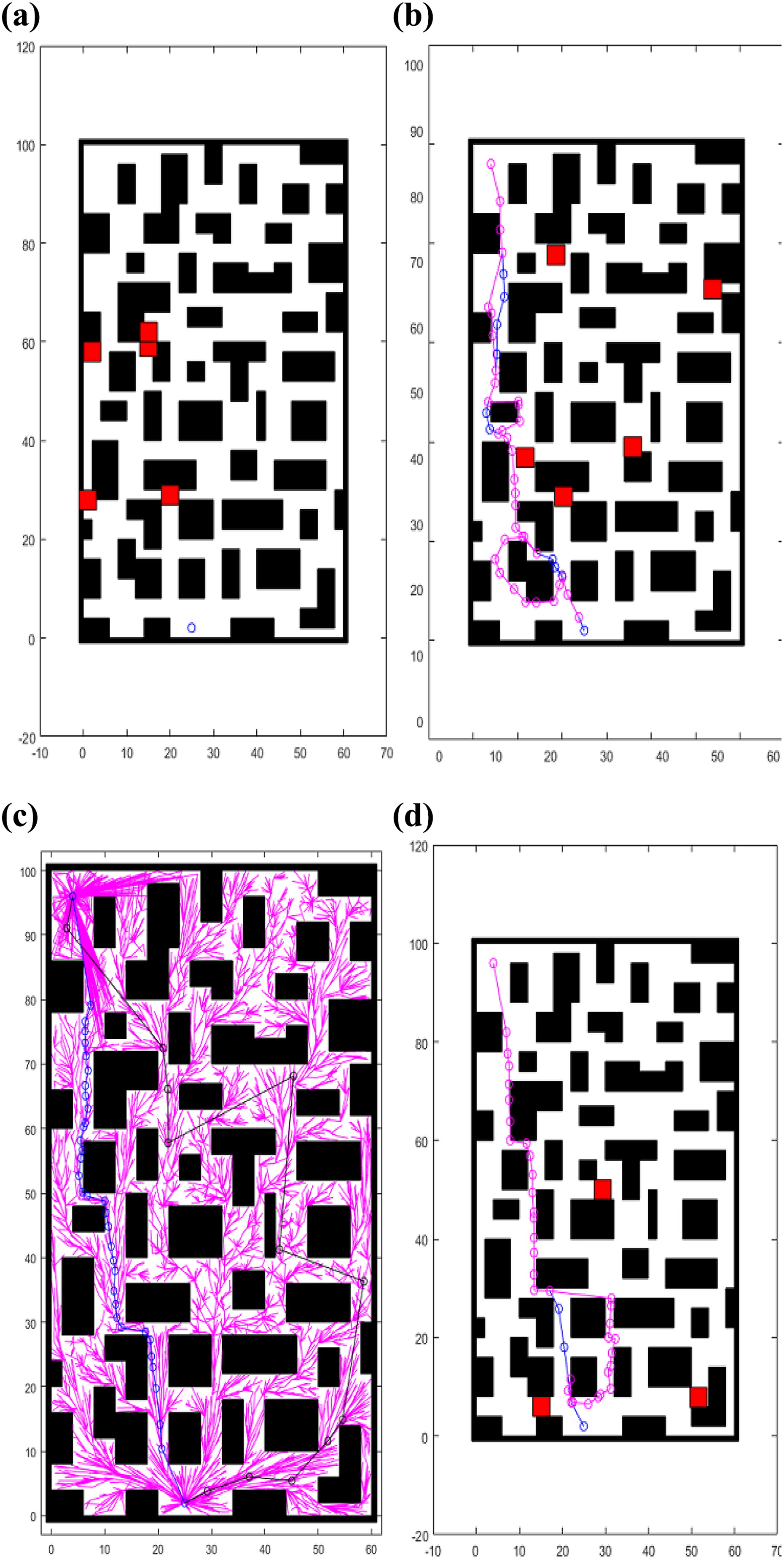
A sample RRT* search tree containing 5000 nodes and replanning results from the second and third sets. (a) Initial positions of the moving obstacles. (b) Final obstacle positions and the executed path. (c) RRT* with 5000 nodes. (d) Final obstacle positions and the executed path. RRT*: extended rapidly exploring random tree.

The simulation results shown below demonstrate the robot’s ability to plan a path around the moving obstacle and reach the goal. Using RRT* during the replanning step allows an efficient path to be found to avoid the moving obstacle and continue on the original optimal path. Since the obstacles move randomly, it is possible for the robot to execute the optimal path and never be obstructed by a moving obstacle. Only examples where the robot did encounter these obstacles are shown.

The first set of results uses a search tree containing 2000 nodes. Upon completion of the search tree, the moving obstacles are placed randomly within the configuration space, and the simulation begins. Figure 5(a) shows the search tree found by the robot upon reaching 2000 nodes.

When executing this path, the robot encounters two random obstacles near the center of the configuration space. One obstacle moves across the path and obstructs the robot. The robot triggers a replanning event at this time. Figure 5(b) shows when the robot encountered the moving obstacles and replanned to avoid them. A second obstacle is nearby and can be seen by the robot and must be considered when replanning. Following the replanning steps in algorithm 6, the robot will select a goal location, then modify the search tree to avoid the obstruction.

Figure 5(c) shows the full modified search tree. There is an obvious empty region of the configuration space where the moving obstacles are located. The absence of branches within this area shows the robot has considered this space as obstacle space, rather than free space. Note, the nodes in this region are not removed; they are considered invalid. If the robot should need to replan again, and this area is free of any moving obstacles, these nodes would be available.

When the robot reaches the replanning goal location, the original path can resume. Figure 5(d) shows the completed path, along with the final positions of the random moving obstacles. The magenta line shows the path followed by the robot. The sections in blue are unexecuted portions of the original path.

The second set of results is similar to the first, with one exception. The random moving obstacle initial positions were selected; in order to increase the probability, the robot would encounter one, or many, while executing the path. Figure 6(a) shows the starting locations of the moving obstacles. The robot was obstructed three times during the execution of the path and successfully planned around the moving obstacle each time. Figure 6(b) shows the final positions of moving obstacles and the path followed by the robot.

The final set of results is a simulation with a search tree containing 5000 nodes and three obstacles moving at random in the configuration space. The three moving obstacles in this simulation were placed similarly to those in the second simulation. In this simulation, the robot encounters a moving obstacle very early in the execution of the path. The robot finds a path around the moving obstacle and completes the path. Figure 6(d) shows the final positions of the obstacles and the executed path.

Multi-robot path planning

In some scenarios, the use of multiple robots will accomplish a task far more efficiently than a single robot. A task may be to obtain sensor readings, build a scalar field map (20; 18), or search a building for people. In these scenarios, each robot will have a starting position and a goal position. With each robot operating in the same environment, the ability to share path planning and search tree information is valuable. The following section presents a method of information sharing in which nodes within each robot’s search tree are shared among nearby robots in order to obtain path planning results more efficiently.

Node description

The nodes, or vertices, used in an RRT search tree must maintain more information than position. Each must store which node is the parent within the tree. The node must also maintain its cost in order to determine an optimal path. When using RRT*, the nodes may also manage a list of nodes within its neighborhood. The list of nearby nodes is used for rewiring in order to reduce cost when new nodes are added to the tree.

Multi-robot RRT*

The extension of RRT* to be used by multiple robots is at its core of the single robot version of RRT*. The difference is a few extra steps during the construction of the search tree. The search is paused in order to share nodes between other robots in communication range. Algorithm 7, below, describes the method for using RRT* with multiple robots. The primary functions in the algorithm are the same as the RRT* functions described in algorithm 1 in “RRT and RRT*-based robot path planning” section. The algorithm will continue to add nodes until the maximum number is reached (see line 3 of algorithm 7). Adding nodes to the tree using RRT* is broken up into steps. Each robot will add a predetermined number of nodes to their own trees using the same method as RRT* (see lines 4–10 of algorithm 7). The next step is to share the newly added nodes with each robot in communication range. When this is complete, the nodes received from other robots are added to the tree. The total number of nodes is then updated and the process continues until the maximum number of nodes is reached.

Algorithm 7

T ← MultiRobotRRT*().

Node sharing

Node sharing will only be executed with robots that are in communication range of each other. In the results below, the communication is controlled by the simulation. The nodes are copied from one robot to a buffer of nodes to be used by the neighboring robot. These nodes are not immediately inserted into the search tree. The robot will wait until all nodes from neighboring robots are transferred before adding them to the tree.

Adding shared nodes using RRT*

The next step is to add the nodes received from neighboring robots to the search tree. First, the entire buffer of shared nodes is appended to the search tree list of nodes. Each of these nodes does not have a parent node and is given a large initial cost. The large cost is used to determine which nodes have a valid connection to the search tree and which do not. Next, beginning with the first shared node, each node is added to the tree using RRT*. Algorithm 8 describes the process for connecting the shared nodes to the tree.

Algorithm 8

AddSharedNodes (T, Q_shared).

First, the node finds all the nodes within its neighborhood (see line 2 of algorithm 8). Next, the node selects the best parent using the $C h o o s e P a r e n t ()$ function (see line 3 of algorithm 8). Once the node is connected to a parent node within the tree, the $R e w i r e ()$ function is called (see line 4 of algorithm 8). As described above, the $R e w i r e ()$ function changes the parent of a nearby node if the cost to reach that node is lower than its current cost. In this case, there may be several nodes in the neighborhood that are not yet connected to the search tree. $R e w i r e ()$ will connect these nodes by giving them a parent and a cost. In some cases, a shared node will be rewired and be connected to the best possible parent. When all the shared nodes are added to the robot’s search tree, the total number of nodes is updated (line 13 of algorithm 7) and the algorithm continues.

Results

The results for the multi-robot path planning method described were gathered in the same manner as the static RRT and RRT* comparison results. In the experiments below, there is a three-robot configuration and a four-robot configuration. There are also two different communication patterns. The first communication pattern is an all-to-all communication pattern where each robot communicates with all other robots. The second communication pattern is restricted to neighboring robots only. For example, in the three robot scenarios, one robot has two neighbors, whereas two robots only have one neighbor. Each robot will build a search tree to satisfy a single-query path plan from its own start and goal location. In the following scenarios, the robots will add 100 nodes to their search tree before sharing those 100 nodes with the other robots.

Scenario 1: In the first multi-robot scenario, there are three robots with an all-to-all communication pattern, shown in Figure 7(a). The robots are allowed a maximum of 1500 nodes in the search tree. Each robot will reach the maximum of 1500 nodes at the same time. Since the robots have perfect communication with each other, the nodes within each search tree will be identical. The path costs and parent nodes will be specific to the individual robot. Figure 8 shows the search trees for each robot.

Figure 7.

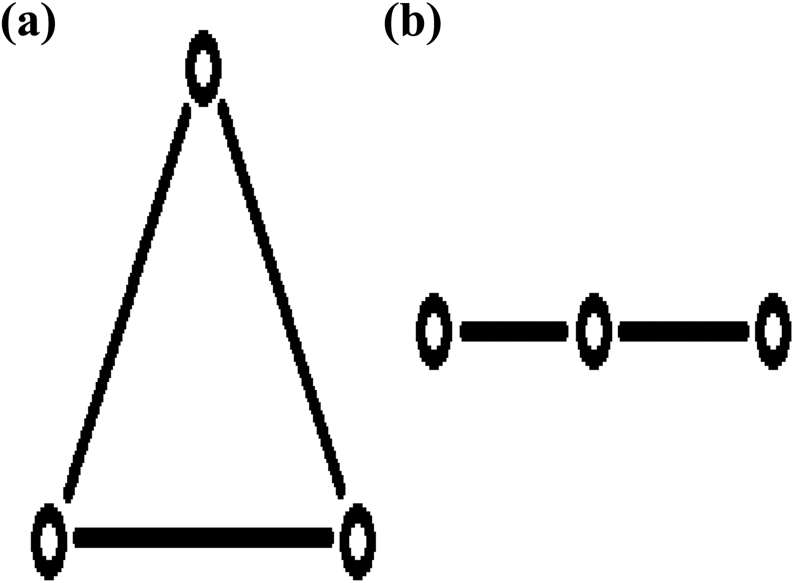
Three robot communication patterns. (a) All-to-all communication pattern. (b) Neighbor-only communication pattern.

Figure 8.

Mulit-robot planning results from the first scenario. (a) Search tree for robot 1. (b) Search tree for robot 2. (c) Search tree for robot 3.

Scenario 2: The second multi-robot scenario has three robots that may only communicate with neighboring robots, shown in Figure 7(b). The center robot, or robot 2, in this scenario completes a 1500 node search tree faster than the other two robots because it receives nodes from two neighbors instead of just one. In order for the other two robots to reach the maximum of 1500 nodes, they must spend extra time adding nodes using RRT* without receiving any new nodes from a neighbor. Figure 9 shows the search tree for each robot. The optimal paths found by each robot are slightly worse than that in scenario 1. Table 1 shows the path costs for each three robot scenario. Robot 2 has the same start and goal locations as the static environment experiments in “Dynamic replanning” section. The optimal paths found in both scenarios 1 and 2 have a similar cost to the static RRT* experiment using 2000 nodes.

Figure 9.

Mulit-robot planning results from the second scenario. (a) Search tree for robot 1. (b) Search tree for robot 2. (c) Search tree for robot 3.

Table 1.

Path costs of three robot scenarios.

Multi-robot path costs
	Robot 1	Robot 2	Robot 3
Scenario 1	112.847	105.185	107.233
Scenario 2	116.652	106.911	108.558

Scenario 3: The third scenario has four robots with an all-to-all communication pattern, shown in Figure 10(a). In this scenario, the robot will add 100 nodes to the tree, then add the 300 nodes received from the neighboring robots. The maximum number of nodes for this scenario was increased to 1600 in order to complete the node sharing process. If the maximum was still 1500, the last 100 shared nodes would not be added to the tree. Figure 11 shows the search tree results.

Figure 10.

Four robot communication patterns. (a) All-to-all communication pattern. (b) Neighbor-only communication pattern.

Figure 11.

Mulit-robot planning results from the third scenario. (a) Search tree for robot 1. (b) Search tree for robot 2. (c) Search tree for robot 3. (d) Search tree for robot 4.

Scenario 4: The fourth scenario has four robots that are only allowed to communicate with their immediate neighbors, shown in Figure 10(b). The communication scheme can be thought of as a square, where each robot occupies a corner. The edges of the square represent the communication links. If the robot numbers are counted clockwise around the square, robot 1 will communicate with robots 2 and 4. In this scenario, each node sharing step will produce 300 nodes for the tree. The maximum number of nodes allowed is 1500 to complete the node sharing process. Figure 12 shows the search tree results for this scenario.

Figure 12.

Mulit-robot planning results from the fourth scenario. (a) Search tree for robot 1. (b) Search tree for robot 2. (c) Search tree for robot 3. (d) Search tree for robot 4.

The overall path quality was better in the third scenario. This was expected since each tree contains 100 more nodes than the fourth scenario. Table 2 shows the path length results from scenarios 3 and 4. Although the trees in scenario 3 are larger, the paths found in scenario 4 are still comparable. Similar to scenarios 1 and 2, the optimal path found for robot 2 is similar or better than the RRT* static environment experiments using a search tree of 2000 nodes. Experiments indicate that sharing node information from multiple robots yields equivalent or better paths with fewer total nodes in an individual search tree.

Table 2.

Path costs of four robot scenarios.

Multi-robot path costs
	Robot 1	Robot 2	Robot 3	Robot 4
Scenario 3	114.254	104.860	106.800	104.864
Scenario 4	117.664	104.877	112.519	113.257

Multi-robot timing results

In addition to compare the quality of the paths found, the execution time to build the search tree was also investigated. In the scenarios above, each individual robot will build a search tree containing the maximum number of nodes. The other option to build these search trees is to have each robot build its own individual search tree. Table 3 shows the average execution time over 10 runs for each method of building a search tree for three robots. The time to build these search trees in scenario 1, where each robot has perfect communication with the other two robots, performed the best. The improvement over building three individual search trees is about 10%. Even scenario 2 performed better than building three separate search trees. In scenario 2, robot 2 will complete a 1500 node search tree faster than its neighbors because it receives nodes from both neighbors. When robot 2 reaches the maximum of 1500 nodes, it will stop discovering new nodes and, therefore, stop sharing nodes with neighboring robots. The other two robots will need to spend extra time completing their search trees without receiving nodes from their neighbor. The extra time spent completing the search trees is why scenario 2 has a lower time performance than scenario 1.

Table 3.

Execution times of three robot scenarios.

Three robot execution times
Robot scenario	Average time (10 simulations)
Individual RRT* search trees	1274.8 s
Multi-robot scenario 1	1144.3 s
Multi-robot scenario 2	1207.8 s

RRT*: extended rapidly exploring random tree.

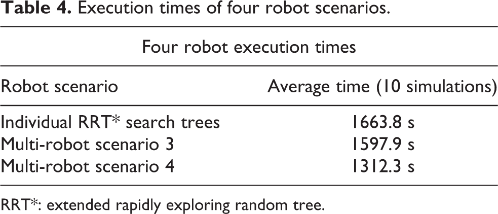
The timing results for the four robot scenarios are similar to the three robot scenarios. Execution times of scenarios 3 and 4 are compared to building four individual search trees. Table 4 shows the average execution time over 10 runs for these scenarios. The timing for each of the multi-robot node sharing experiments is better than building a search tree individually for each robot. Scenario 3 does have search trees with 100 more nodes than scenario 4. There are two other differences between scenarios 3 and 4 that influence the execution time. First, each robot in scenario 3 will receive 100 nodes from each neighbor for a total of 300 at each node sharing step. In scenario 4, each robot receives a total of 200 nodes from the neighboring robots. The second difference is in the number of times that nodes are shared between robots. In scenario 3, the robots will reach the maximum node limit after four iterations of lines 4–13 of algorithm 7. Scenario 4 will reach the maximum node limit after five iterations. Since scenario 3 has a longer execution time, the additional time must be coming from the additional 100 nodes received by each robot during each node sharing step.

Table 4.

Execution times of four robot scenarios.

Four robot execution times
Robot scenario	Average time (10 simulations)
Individual RRT* search trees	1663.8 s
Multi-robot scenario 3	1597.9 s
Multi-robot scenario 4	1312.3 s

RRT*: extended rapidly exploring random tree.

Conclusion and future work

In this article, we presented a new method of dynamic replanning for a mobile robot to avoid unknown and unpredictable moving obstacles. The replanning method leverages the $R e w i r e ()$ function of RRT* in order to modify and expand the existing search tree to avoid a random obstacle when it is detected. As a result, the robot was able to dynamically determine a course of action in order to reach the goal while avoiding both static and moving obstacles. Multiple testing scenarios were conducted to demonstrate the efficiency of this replanning method. We expect that the proposed replanning method is a good first step toward more research on replanning using RRT*.

Additionally, for multi-robot team, a collaborative multi-robot path planning method by sharing nodes between robots is developed. Different multi-robot configurations with both “all-to-all” and “neighboring-only” communication protocols were studied. The results presented indicated that the multi-robot path planning method produces equivalent quality paths in a shorter execution time than building multiple individual search trees using RRT*.

There are several options for future research on the topic of dynamic replanning. Future work will research a floating replan goal location to minimize the total remaining cost to the query goal. Minimizing the modifications to the original search tree is another area of improvement. This method has only been implemented in a 2-D configuration space. The algorithm should be further expanded and modified to operate in higher dimension configuration spaces. The simulations up to this point have been with small numbers of moving obstacles; further research is needed to determine how the algorithm performs when there are many random moving obstacles.

Multi-robot path planning also requires additional research. Future work will research increasing the number of robots in the multi-robot team. Additional research is needed to maximize the number of shared nodes while minimizing execution time to add the shared nodes to the tree. Another area of future work is comparing multi-robot results to single robot results when a larger search tree is used by the single robot. Finally, more research is needed using sensors to detect the environment and dynamic communication. Sensors will limit how much of the environment the robot is able to explore and share with neighboring robots. Dynamic communication will represent a realistic communication scheme where robots will move in and out of communication range. Additional research is pursuing multi-robot systems. Efficient path planning and replanning will benefit cooperative multi-agent sensing systems,^{21,22, 29} cooperative learning³⁰ and formation control systems,^23

–27 and target tracking and observation.^28,31,32

Footnotes

Declaration of conflicting interests

The author(s) declared no potential conflicts of interest with respect to the research, authorship, and/or publication of this article.

Funding

The author(s) disclosed receipt of the following financial support for the research, authorship, and/or publication of this article: This work was partially supported by the National Aeronautics and Space Administration (NASA) under grant number NNX15AI02H issued through the Nevada NASA Research Infrastructure Development Seed Grant, and the National Science Foundation (IIS-NRI 1426828). This work was also supported by the U.S. Department of Transportation, Office of the Assistant Secretary for Research and Technology (USDOT/OST-R) under grant number 69A3551747126 through INSPIRE University Transportation Center () at Missouri University of Science and Technology. The views, opinions, findings and conclusions reflected in this publication are solely those of the authors and do not represent the official policy or position of the USDOT/OST-R, or any State or other entity.

References

Kavraki

Svestka

Latombe

. Probabilistic roadmaps for path planning in high-dimensional configuration spaces. IEEE Trans Rob Autom 1996; 12(4): 566–580.

Lavalle

. Rapidly-exploring random trees: a new tool for path planning. Tech rep 1998: 1–4.

Karaman

Frazzoli

. Optimal kinodynamic motion planning using incremental sampling-based methods. In: 49th IEEE conference on decision and control (CDC), Atlanta, GA, USA, 15–17 December 2010, pp. 7681–7687, IEEE.

Karaman

Walter

Perez

. Anytime motion planning using the RRT*. In: 2011 IEEE international conference on robotics and automation, Shanghai, China, 9-13 May 2011, pp. 1478–1483, IEEE.

Ferguson

Stentz

. Anytime RRTs. In: 2006 IEEE/RSJ international conference on intelligent robots and systems, Beijing, China, 9–15 October 2006, pp. 5369–5375, IEEE.

Karaman

Frazzoli

. Sampling-based algorithms for optimal motion planning. Int J Rob Res 2011; 30(7):846–894.

Perez

Platt

Konidaris

. LQR-RRT*: optimal sampling-based motion planning with automatically derived extension heuristics. In: 2012 IEEE international conference on robotics and automation, Saint Paul, MN, USA, 14–18 May 2012, pp. 2537–2542, IEEE.

Gammell

Srinivasa

Barfoot

. Informed RRT*: optimal sampling-based path planning focused via direct sampling of an admissible ellipsoidal heuristic. In: 2014 IEEE/RSJ international conference on intelligent robots and systems, Chicago, IL, USA, 14–18 September 2014, pp. 2997–3004, IEEE.

Salzman

Halperin

Asymptotically near-optimal RRT for fast, high-quality, motion planning. In: 2014 IEEE international conference on robotics and automation (ICRA), Hong Kong, China, 31 May–7 June 2014, pp. 4680–4685.

10.

Islam

Nasir

Malik

. RRT*-smart: rapid convergence implementation of RRT*; towards optimal solution. In: 2012 IEEE international conference on mechatronics and automation, Chengdu, China, 5–8 August 2012, pp. 1651–1656, IEEE.

11.

Qureshi

Iqbal

Qamar

. Potential guided directional-RRT* for accelerated motion planning in cluttered environments. In: 2013 IEEE international conference on mechatronics and automation, Takamatsu, Japan, 4–7 August. 2013, pp. 519–524, IEEE.

12.

Gibb

Pham

. Autonomous robotic system using non-destructive evaluation methods for bridge deck inspection. In: 2017 IEEE international conference on robotics and automation (ICRA), Singapore, 29 May–3 June 2017, pp. 3672–3677, IEEE.

13.

Woods

. A novel potential field controller for use on aerial robots. IEEE Transactions on Systems, Man, and Cybernetics: Systems 2017: 1–12.

14.

Gucunski

Kee

. Autonomous robotic system for bridge deck data collection and analysis. In: 2014 IEEE/RSJ international conference on intelligent robots and systems, Chicago, IL, USA, 14–18 September. 2014, pp. 1950–1955, IEEE.

15.

Lim

Basily

. Mechatronic systems design for an autonomous robotic system for high-efficiency bridge deck inspection and evaluation. IEEE ASME Trans Mechatron 2013; 18(6): 1655–1664.

16.

Connell

HM.

Dynamic path planning and replanning for mobile robots using RRT*. In: 2017 IEEE international conference on systems, man, and cybernetics (SMC), Banff, AB, Canada, 5–8 October 2017, IEEE.

17.

Bruce

Veloso

. Real-time randomized path planning for robot navigation. In: IEEE/RSJ international conference on intelligent robots and systems, Lausanne, Switzerland, 30 September – 4 October 2002, Vol. 3. pp. 2383–2388 IEEE.

18.

Ferguson

Kalra

Stentz

. Replanning with RRTs. In: Proceedings 2006 IEEE international conference on robotics and automation, 2006, ICRA 2006. Orlando, FL, USA, 15–19 May 2006, pp. 1243–1248, IEEE.

19.

Zucker

Kuffner

Branicky

. Multipartite RRTs for rapid replanning in dynamic environments. In: Proceedings 2007 IEEE international conference on robotics and automation, Roma, Italy, 10-14 April 2007, pp. 1603–1609, IEEE.

20.

Otte

Frazzoli

RRTx: asymptotically optimal single-query sampling-based motion planning with quick replanning. Int J Rob Res 2016; 35(7): 797–822.

21.

Sheng

Chen

. Cooperative and active sensing in mobile sensor networks for scalar field mapping. IEEE Trans Syst Man Cybern Syst 2015;45(1): 680–691.

22.

Sheng

. Distributed sensor fusion for scalar field mapping using mobile sensor networks. IEEE Trans Cybern 2013; 43(2): 766–778.

23.

Nguyen

Jafari

. Formation control and obstacle avoidance of multiple rectangular agents with limited communication ranges. IEEE Trans Control Network Syst 2017; 4(4): 1.

24.

Lim

Sheng

. Cooperative flocking and learning in multi-robot systems for predator avoidance. In: 2013 IEEE international conference on cyber technology in automation, control and intelligent systems, Nanjing, China, 26–29 May 2013, pp. 337–342, IEEE.

25.

Sheng

. Multi-agent motion control in cluttered and noisy environments. J Commun 2013; 8(1): 32–46.

26.

Dang

Manh La

Horn

. Distributed formation control for autonomous robots following desired shapes in noisy environment. In: 2016 IEEE international conference on multisensor fusion and integration for intelligent systems (MFI), Baden-Baden, Germany, 19–21 September 2016, pp. 285–290, IEEE.

27.

Sheng

. Flocking control of multiple agents in noisy environments. In: 2010 IEEE international conference on robotics and automation, Anchorage, AK, USA, 3–7 May 2010, pp. 4964–4969, IEEE.

28.

Sheng

. Dynamic targets tracking and observing in a mobile sensor network. Elsevier J Robot Autonomous Syst 2012; 60(7): 996–1009.

29.

Nguyen

Teague

. Collaborative and compressed mobile sensing for data collection in distributed robotic networks. IEEE Transactions on Control of Network Systems 2017: 1.

30.

Lim

Sheng

. Multirobot cooperative learning for predator avoidance. IEEE Trans Control Syst Technol 2015; 23(1): 52–63.

31.

Pham

Feil-Seifer

. A distributed control framework of multiple unmanned aerial vehicles for dynamic wildfire tracking. IEEE Transactions on Systems, Man, and Cybernetics: Systems 2018: 1–12.

32.

Pham

Feil-Seifer

. A distributed control framework for a team of unmanned aerial vehicles for dynamic wildfire tracking. In: 2017 IEEE/RSJ international conference on intelligent robots and systems (IROS), Vancouver, BC, Canada, 24–28 September. 2017, pp. 6648–6653, IEEE.

Extended rapidly exploring random tree–based dynamic path planning and replanning for mobile robots

Abstract

Keywords

Introduction

RRT and RRT*-based robot path planning

Comparison results

Statistical comparison results

Dynamic replanning

Open problem

Path execution

Random moving obstacles and detection

Path replanning

Path obstruction

Establish replanning goal location

Modify search tree

Subpath selection and execution

Results

Multi-robot path planning

Node description

Multi-robot RRT*

Node sharing

Adding shared nodes using RRT*

Results

Multi-robot timing results

Conclusion and future work

Footnotes

Declaration of conflicting interests

Funding

References