Three-dimensional multi-robot control to chase a target while not being observed

Abstract

This article introduces a 3-D multi-robot chasing controller to make a team of robots get closer to a target while not being observed by the target. Assume that the target has sensors, such as radar or sonar, to observe an incoming vehicle. In the team, one robot, the leader, has a stealth capability such that it is not observable by the sensors of the target while getting closer to the target. The leader is controlled such that it chases the target while remaining at the same bearing line from the target to the leader. Considering the case in which the target can only measure optical flow, the target can hardly observe the leader’s motion. We control every robot, other than the leader, such that a detection pulse signal generated from the target’s sensor reaches no robot, since the signal is attenuated by the stealth leader. In this manner, even if multiple robots approach the target, the target observes no robot. We prove that under our 3-D multi-agent control with some condition satisfied, multiple robots can approach the target in a stealthy manner while avoiding colliding with each other. In this article, we use simulations to demonstrate the effectiveness of our 3-D multi-agent controller.

Introduction

Recently, stealth vehicles are built, employing stealth technology so that they are harder to be observed by sensors, such as radar or sonar. A stealth vehicle can absorb a detection pulse signal generated from sensors, such as radar or sonar. ¹

Consider the problem of employing a team of robots for chasing a target. ^{2 –6} This article considers a scenario of making multiple robots get closer to a target while not being observed by the target. Usually, a robot with stealth technology is expensive. Thus, utilizing many stealth vehicles is not desirable considering cost.

This article presents a 3-D multi-robot chasing controller to make a team of robots get closer to a target while not being observed by the target. The target has sensors, such as radar or sonar, to observe an incoming vehicle. Among the team members, one robot, the leader, has a stealth capability such that it is not observable by the target’s sensor while getting closer to the target.

The leader is controlled such that it gets closer to the target while remaining at the same bearing line from the target to the leader. Many insects and animals utilize this motion camouflage control to chase their prey. ^{7 –10} Considering the case in which the prey can only measure optical flow, this motion by the pursuer is hardly observable by the prey. ¹⁰

Reddy et al. ¹¹ developed a 3-D controller to perform this kind of motion camouflage. Under the controller, ¹¹ it was proved that the pursuer converges to the motion camouflage state in three dimensions. In this article, the controller in the study by Reddy et al. ¹¹ is utilized to control the leader.

The leader is a stealth vehicle such that the target’s sensor cannot measure the leader’s position. We acknowledge that the types of stealth vehicles currently being built are underactuated vehicles, such as submarines and airplanes. These underactuated vehicles have kinematic and dynamic constraints on their motion. Since the controller in the study by Reddy et al. ¹¹ was developed considering a holonomic vehicle, the controller ¹¹ may not be able to make the leader converge to the motion camouflage state in the case where the leader is an underactuated vehicle.

Note that we can build a holonomic stealth vehicle by making a holonomic vehicle absorb a detection pulse signal. ¹ This article assumes that every vehicle is a holonomic vehicle. In fact, this holonomic vehicle assumption is commonly utilized in many papers on multi-robot systems. ^{12 –19}

We control every robot, other than the leader, such that a detection pulse signal generated from the target reaches no robot, since the signal is attenuated by the stealth leader. In this manner, even if multiple robots approach the target, the target observes no robot. Let a follower denote a robot that is not the leader. Each follower is controlled such that it converges to the bearing line connecting the target and the leader while getting closer to the target. In this manner, a follower can “hide” behind the stealth leader while approaching the target. This article proves that under the proposed 3-D chasing controller, a follower approaches the target while not being observed by the target.

There are many papers on multi-robot systems. ^{12 –23} Multi-robot systems have various potential applications such as leader-based multi-robot herding, ²⁴ sensor node deployment, ^{12,20,21,23,25} and collective transport of robots. ²⁶ Zhang and Leonard ¹⁸ developed formation controllers to improve source seeking utilizing distributed sensors. Previous studies ^{2 –6} considered the problem of employing a team of robots for tracking one or more targets. Researchers ^2,5 handled cooperative control of a team of robots to estimate the position of a moving target. Our article proposes 3-D control laws to make multiple robots get closer to the target while not being observed by the target. As far as we know, this kind of multi-agent control in 3-D environments has not been handled in the literature on multi-agent systems.

Various controllers have been developed to make a vehicle track a path. ^{27 –29} Line-of-sight (LOS) guidance controller has been widely utilized to make the vehicle follow a path in a robust manner. ^27,29 LOS guidance controller was developed to make the vehicle converge to the path in the case where the cross-track error (the distance to the path) is not zero. Our multi-robot chasing controller is developed inspired by LOS guidance controllers. ^{27 –30}

In our multi-agent control laws, the leader and followers utilize sensors, such as GPS, to localize themselves, respectively. Also, the leader information (position and velocity) is transmitted to every follower so that each follower can predict the leader location after one-time step in the future.

In our multi-agent control laws, the leader utilizes various sensors, such as radar or sonar, to access the target position in real time. The leader then predicts the target location within one time step in the future. Prediction of target’s location is not easy, since it is associated to the target’s maneuvers. Moreover, sensor measurement noise exists as the pursuer measures the target’s location in real time. Third section thus introduces a curve fitting approach to predict the target’s location one step forward in time considering noisy sensor measurements.

We prove that under our 3-D multi-agent control laws, a robot can get sufficiently close to the target while not being observed by the target. Collision avoidance must be assured as multiple robots approach the target. Thus, this article proves that under our 3-D multi-agent control with some condition satisfied, multiple robots avoid colliding with each other. Simulations are utilized to demonstrate the effectiveness of our 3-D multi-agent controller.

The article is organized as follows: second section introduces assumptions and definitions in our article. Third section introduces a curve fitting approach to predict the target’s location one step forward in time considering noisy sensor measurements. Fourth section presents the proposed 3-D multi-agent controller. Fifth section introduces simulations to demonstrate the effectiveness of our 3-D multi-agent controller. Sixth section presents conclusions.

Assumptions and definitions

We discuss assumptions and definitions utilized in this article. This article considers a team of robots composed of one leader and one or more followers in 3-D. $v^{\mathbf{l}}$ is the leader’s speed, and v^f is a follower’s speed. v^t is the speed of the target. In this article, each robot in 3-D is simplified as a sphere. $R^{\mathbf{l}}$ is the leader’s radius. Also, R^f is a follower’s radius.

In the team, the leader has a stealth capability such that it is not detected by sensors, such as sonar or radar, while getting closer to the target. The leader is controlled such that it chases the target while remaining at the same bearing line from the target to the leader. To control the motion of the leader, we use the 3-D chasing control law in Reddy et al.’s study. ¹¹

To simulate the motion of the target, we use Frenet–Serret frames, ^11,31 Which is discussed in the fifth section.

The purpose of our article is as follows: design controllers for each follower so that each follower get sufficiently close to the target in an unobservable manner, so that the robot can monitor the target state closely. We assume that $v^t<v^{\mathbf{l}}$ and that $v^t<v^f$ . We further assume that the sensing range of each follower is bigger than $(v^f+v^t)T$ . Here, T is the sampling time interval of our 3-D chasing controllers. Once the distance between the target and a follower is less than $(v^f+v^t)T$ , then the follower can monitor the target state utilizing on-board sensors. Thus, we develop a follower’s controller so that the distance between the target and the follower decreases to be less than $(v^f+v^t)T$ , while the follower is not observed by the target.

Suppose that there are N followers. Fⁱ is the i th follower, where $i\le N$ . L is the infinite line intersecting both the target and the leader.

The subscript k is utilized to represent the time index k in discrete-time systems. ${\mathbf{f}}_k^i$ is the 3-D location of Fⁱ at k th time index. ${\mathbf{t}}_k$ is the target’s 3D location at k th time index, and ${\mathbf{l}}_k$ is the leader’s 3-D location at k th time index. $L_k$ represents the infinite line intersecting both ${\mathbf{t}}_k$ and ${\mathbf{l}}_k$ .

Since a follower can predict both ${\mathbf{t}}_{k+1}$ and ${\mathbf{l}}_{k+1}$ , a follower can access $L_{k+1}$ . ${\mathbf{c}}_k^i$ is the 3-D point on $L_{k+1}$ , which is the closest to ${\mathbf{f}}_k^i$ . Also, $d_k^i$ is $\parallel {\mathbf{f}}_k^i-{\mathbf{c}}_k^i\parallel$ . $\angle ({\mathbf{v}}_1,{\mathbf{v}}_2)$ is the angle formed by ${\mathbf{v}}_1$ and ${\mathbf{v}}_2$ . In other words, $\angle ({\mathbf{v}}_1,{\mathbf{v}}_2)=\text{arccos}(\frac{{\mathbf{v}}_1\cdot {\mathbf{v}}_2}{\parallel {\mathbf{v}}_1\parallel \parallel {\mathbf{v}}_2\parallel })$ . Here, $\angle ({\mathbf{v}}_1,{\mathbf{v}}_2)$ exists between 0 and π, satisfying that $\text{sin}\left(\angle ({\mathbf{v}}_1,{\mathbf{v}}_2)\right)>0$ .

${\mathbf{h}}_k^i$ denotes the heading point of Fⁱ at time step k. This implies that at each time step k, Fⁱ heads toward ${\mathbf{h}}_k^i$ . The definition of ${\mathbf{h}}_k^i$ in the situation where $d_k^i>v^{\mathbf{f}}T$ is distinct from that of ${\mathbf{h}}_k^i$ in the situation where $d_k^i\le v^{\mathbf{f}}T$ . In the situation where $d_k^i>v^{\mathbf{f}}T$ , ${\mathbf{h}}_k^i$ is defined as ${\mathbf{c}}_k^i$ . In the situation where $d_k^i\le v^{\mathbf{f}}T$ , ${\mathbf{h}}_k^i$ is defined as the point on $L_{k+1}$ , which is $\sqrt{{(v^{\mathbf{f}}T)}^2-{(d_k^i)}^2}$ distance from ${\mathbf{c}}_k^i$ and is on the line segment whose two end points are ${\mathbf{c}}_k^i$ and ${\mathbf{t}}_{k+1}$ , respectively. Figure 1 illustrates ${\mathbf{h}}_k^i$ in the situation where $d_k^i\le v^{\mathbf{f}}T$ .

Figure 1.

In the situation where $d_k^i\le v^{\mathbf{f}}T$ , ${\mathbf{f}}_{k+1}^i$ is on $L_{k+1}$ .

We say that collision avoidance between two vehicles is assured if the relative distance between the two vehicles is bigger than $C_d$ . This implies that $C_d$ denotes the minimum separation between two vehicles for collision avoidance.

Conditions for unobservable state

Among all robots, only the leader has a stealth capability such that it is not observed by the target’s sensors while chasing the target. Every robot, other than the leader, is controlled such that a detection pulse signal generated from the target’s sensor reaches no robot, since the signal is attenuated by the leader. In this manner, the target observes no robot while multiple robots chase the target.

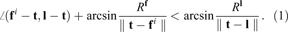
Considering the volume of each robot, a detection pulse signal generated from the target cannot reach Fⁱ if the below condition is met.

$\angle ({\mathbf{f}}^i-\mathbf{t},\mathbf{l}-\mathbf{t})+\text{arcsin}\frac{R^{\mathbf{f}}}{\parallel \mathbf{t}-{\mathbf{f}}^i\parallel }<\text{arcsin}\frac{R^{\mathbf{l}}}{\parallel \mathbf{t}-\mathbf{l}\parallel }\mathrm{.}$

1

Fⁱ is unobservable if equation (1) is met. If equation (1) is met at k th time index, then we say that Fⁱ is in the unobservable state S_s at k th time index. This indicates that Fⁱ is not observable by the target’s sensor while Fⁱ chases the target.

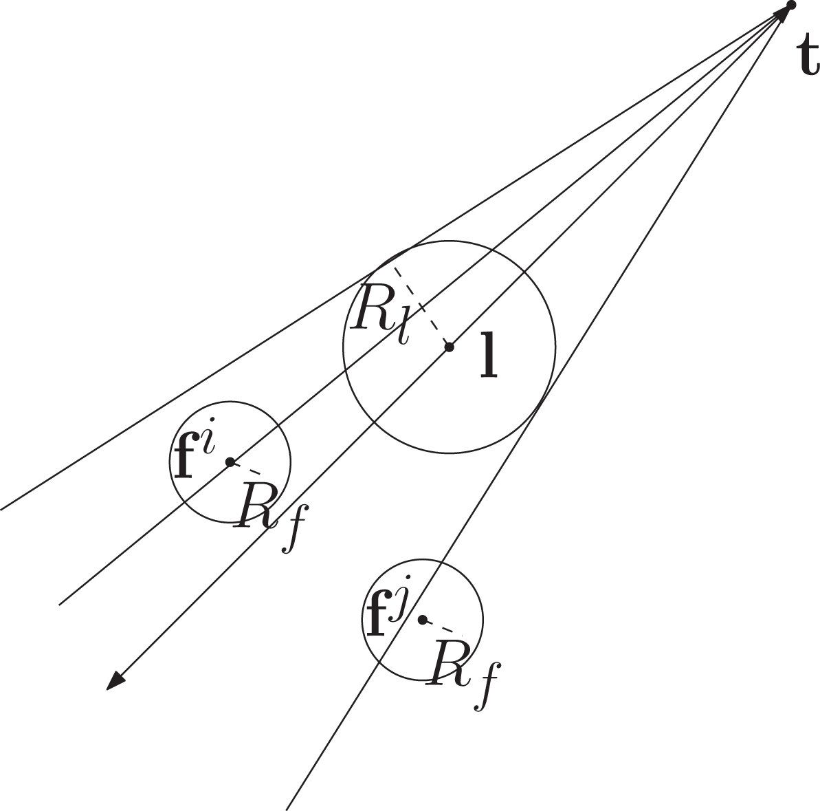
Figure 2 illustrates the situation in which Fⁱ is unobservable. A detection pulse signal generated from the target cannot reach Fⁱ, attenuated by the leader. Therefore, Fⁱ is not observable by the target’s sensor. But, F^j is observable by the target’s sensor, due to the fact that a detection pulse signal can reach F^j.

Figure 2.

Fⁱ is in the unobservable state. But, F^j is observable by the target’s sensor.

Predict the target position one step forward in time considering noisy environments

The leader uses sensor measurements to derive the target’s location in real time. Then, the leader at time step k predicts ${\mathbf{t}}_{k+1}$ using the curve fitting method in this section.

Prediction of ${\mathbf{t}}_{k+1}$

We utilize curve fitting methods for recent target positions: $\left(x_{k-K+1},y_{k-K+1},z_{k-K+1}\right),\left(x_{k-K+2},y_{k-K+2},z_{k-K+2}\right),\mathrm{\dots },\left(x_k,y_k,z_k\right)$ . Here, $K>2$ . This indicates that we need more than two measurements.

Recent x coordinate of the target are as follows. $x_{k-K+1},x_{k-K+2},\mathrm{...},x_k$ . We fit $x_{k-K+1},x_{k-K+2},\mathrm{...},x_k$ using the following second-order polynomials: $x_n=a_x{(n-k)}^2+b_x(n-k)+{\mathbf{c}}_x$ . This second-order polynomials represent the x coordinate trajectory of the target within recent K time steps.

We utilize the following matrix to solve this curve fitting problem

$A\times S=B$

2

Here, $A=\left(\begin{array}{ccc}{(-K+1)}^2& -K+1& 1\\ {(-K+2)}^2& -K+2& 1\\ \mathrm{...}& \mathrm{...}& \mathrm{...}\\ 0& 0& 1\end{array}\right)$ ,

$B={\left(x_{k-K+1}\mathrm{,}{x}_{k-K+2}\mathrm{,}\mathrm{...}{x}_k\right)}^{\text{T}},\text{ and} S={\left(a_x\mathrm{,}\hspace{0.17em}\hspace{0.17em}{b}_x\mathrm{,}\hspace{0.17em}\hspace{0.17em}{c}_x\right)}^{\text{T}}.$

We solve for S using pseudo-inverse methods as follows

$S={\left(A^{\text{T}}\times A\right)}^{-1}\times A\times B$

3

${\widehat{\mathbf{t}}}_{k+1}$ is the estimate of ${\mathbf{t}}_{k+1}$ . Let ${\widehat{\mathbf{t}}}_{k+1}(j)$ denote the j th element in ${\widehat{\mathbf{t}}}_{k+1}$ . Since $x_n=a_x\times {(n-k)}^2+b_x\times (n-k)+{\mathbf{c}}_x$ , $x_{k+1}=a_x+b_x+{\mathbf{c}}_x$ . Thus, we predict the x coordinate of ${\widehat{\mathbf{t}}}_{k+1}$ as follows

${\widehat{\mathbf{t}}}_{k+1}(1)=Q_2\times S$

4

where $Q_2=\left(1,\hspace{0.17em}1,\hspace{0.17em}1\right)$ .

Similarly, we can estimate the y coordinates of ${\mathbf{t}}_{k+1}$ using the following second-order polynomials: $y_n=a_y{(n-k)}^2+b_y(n-k)+{\mathbf{c}}_y$ . Also, we can estimate the z coordinates of ${\mathbf{t}}_{k+1}$ using the following second-order polynomials: $z_n=a_z{(n-k)}^2+b_z(n-k)+{\mathbf{c}}_z$ . This curve fitting approach requires more than two measurements. In other words, we need $K>2$ . Since the target has been moving before time step 0, we have more than one measurement.

If we have only two measurements ( $k=2$ ), then we set

${\widehat{\mathbf{t}}}_3=(x_1,y_1,z_1)+\mathbf{D}\times 2\times T$

5

where $\mathbf{D}=\frac{(x_2-x_1,y_2-y_1,z_2-z_1)}{T}$ . Equation (5) indicates that we fit two measurements using the first-order polynomials.

The multi-agent controller

In this section, we discuss our 3-D multi-agent controller in detail. At each time index k, the controller for Fⁱ is as follows

${\mathbf{f}}_{k+1}^i={\mathbf{f}}_k^i+v^{f}T\frac{{\mathbf{h}}_k^i-{\mathbf{f}}_k^i}{\parallel {\mathbf{h}}_k^i-{\mathbf{f}}_k^i\parallel }\mathrm{.}$

6

The above controller implies that Fⁱ moves toward its associated heading point ${\mathbf{h}}_k^i$ at each time step k. Since ${\mathbf{h}}_k^i$ exists on $L_{k+1}$ and is on the line segment whose two end points are ${\mathbf{c}}_k^i$ and ${\mathbf{t}}_{k+1}$ , respectively, Fⁱ gets closer to both $L_{k+1}$ and the target. In the situation where $d_k^i>v^{\mathbf{f}}T$ , Fⁱ moves toward $L_{k+1}$ . Figure 3 illustrates this situation. This implies that a follower moves to “hide” behind the leader as fast as possible. In the situation where $d_k^i\le v^{\mathbf{f}}T$ , ${\mathbf{f}}_{k+1}^i$ is on $L_{k+1}$ . Figure 1 illustrates this situation. This implies that a follower “hides” behind the leader completely.

Figure 3.

In the situation where $d_k^i>v^{\mathbf{f}}T$ , ${\mathbf{f}}_{k+1}^i$ is not on $L_{k+1}$ .

We next present the analysis of the proposed controller. In this analysis, we do not consider target prediction error presented in the third section. In other words, we assume that the predicted target state ${\widehat{\mathbf{t}}}_{k+1}$ is identical to the true target state ${\mathbf{t}}_{k+1}$ .

Stability analysis

Under our 3-D multi-agent controller (equation (6)), each follower gets closer to L while chasing the target. See Figures 1 and 3. Since a follower gets closer to L, we encounter a situation where $d_{k^i}^i\le v^{\mathbf{f}}T$ at a certain time step kⁱ. (Assume that all robots are positioned close to each other initially. For instance, we can consider the case where all robots are launched from one platform, such as a submarine or an airplane. In this case, $d_0^i\le v^{\mathbf{f}}T$ is feasible for all $i\le N$ . Hence, it is feasible that kⁱ is zero for all $i\le N$ .)

Once $d_{k^i}^i\le v^{\mathbf{f}}T$ occurs, ${\mathbf{f}}_k^i$ is on L_k for all $k>k^i$ under our 3-D multi-agent controller (6). This is presented as the following theorem.

Theorem 1

Consider the situation where $d_{k^i}^i\le v^{\mathbf{f}}T$ at a certain time step kⁱ. Then, ${\mathbf{f}}_k^i$ is on L_k for all $k>k^i$ . Furthermore, $\parallel {\mathbf{f}}_k^i-{\mathbf{c}}_k^i\parallel \le v^{\mathbf{f}}T$ for all $k>k^i$

Proof

Consider the situation where $d_{k^i}^i\le v^{\mathbf{f}}T$ . In this situation, ${\mathbf{f}}_{k^i+1}^i$ is on $L_{k^i+1}$ under our multi-agent controller (6). See Figure 1.

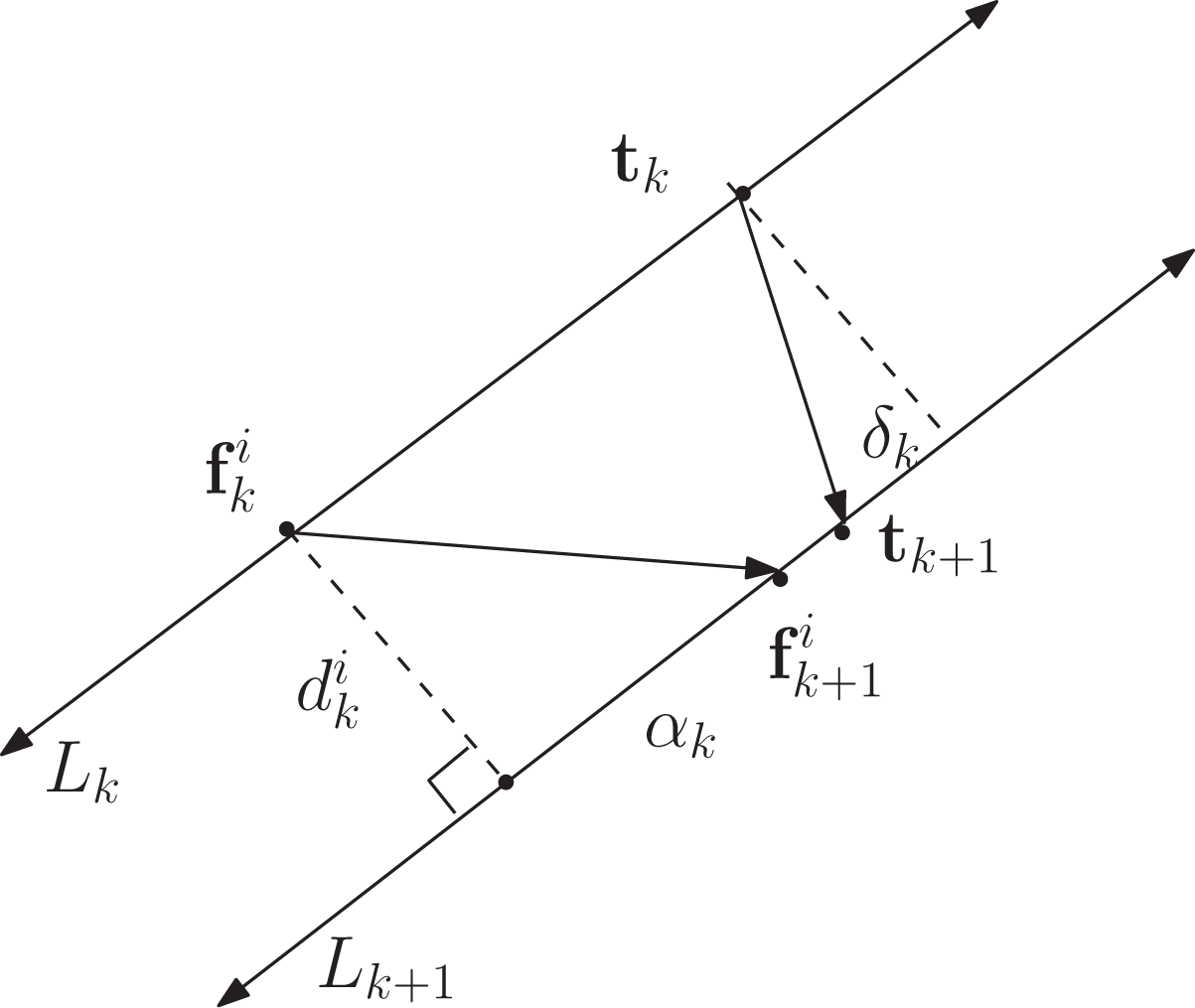
Induction is utilized for our proof. Consider the situation where $k>k^i$ . Suppose that ${\mathbf{f}}_{k+1}^i$ is on $L_{k+1}$ . It is next proved that $\parallel {\mathbf{f}}_{k+1}^i-{\mathbf{c}}_{k+1}^i\parallel \le v^{\mathbf{f}}T$ and that ${\mathbf{f}}_{k+2}^i$ is on $L_{k+2}$ .

$L_{k+2}$ is parallel to $L_{k+1}$ . $\parallel {\mathbf{f}}_{k+1}^i-{\mathbf{c}}_{k+1}^i\parallel$ is the distance between $L_{k+1}$ and $L_{k+2}$ . The target located at $L_{k+1}$ reaches $L_{k+2}$ within one time interval. It is assumed that $v^{\mathbf{t}}<v^{\mathbf{l}}$ and that $v^{\mathbf{t}}<v^{\mathbf{f}}$ . Therefore, $\parallel {\mathbf{f}}_{k+1}^i-{\mathbf{c}}_{k+1}^i\parallel \le v^{\mathbf{t}}T<v^{\mathbf{f}}T$ . In this situation, ${\mathbf{f}}_{k+2}^i$ is on $L_{k+2}$ under our 3-D multi-agent controller (6).

Utilizing induction, we proved that ${\mathbf{f}}_k^i$ is on L_k and that $\parallel {\mathbf{f}}_k^i-{\mathbf{c}}_k^i\parallel \le v^{\mathbf{f}}T$ for all $k>k^i$ . □

Theorem 1 proved that if $d_{k^i}^i\le v^{\mathbf{f}}T$ at a certain time step kⁱ, then ${\mathbf{f}}_k^i$ is on L_k for all $k>k^i$ under our 3-D multi-agent controller (equation (6)). This implies that a follower “hides” behind the leader completely. Note that even if a follower “hides” behind the leader completely, the follower may be detected by the target depending on the size of the follower. We have Theorem 2 to discuss the condition for becoming unobservable.

Theorem 2

Consider the situation where $d_{k^i}^i\le v^{\mathbf{f}}T$ at a certain time step kⁱ. Under our 3-D multi-agent controller (6), Fⁱ at time index $k>k^i$ is unobservable if $\frac{R^{\mathbf{f}}}{\parallel {\mathbf{t}}_k-{\mathbf{f}}_k^i\parallel }<\frac{R^{\mathbf{l}}}{\parallel {\mathbf{t}}_k-{\mathbf{l}}_k\parallel }$ .

Proof

Fⁱ is unobservable if equation (1) is satisfied. Consider the situation where $d_{k^i}^i\le v^{\mathbf{f}}T$ . ${\mathbf{f}}_k^i$ is on L_k for all $k>k^i$ utilizing Theorem 1. Furthermore, $\parallel {\mathbf{f}}_k^i-{\mathbf{c}}_k^i\parallel \le v^{\mathbf{f}}T$ for all $k>k^i$ utilizing Theorem 1.

Since $\parallel {\mathbf{f}}_k^i-{\mathbf{c}}_k^i\parallel \le v^{\mathbf{f}}T$ for all $k>k^i$ , $\angle ({\mathbf{f}}_k^i-{\mathbf{t}}_k,{\mathbf{l}}_k-{\mathbf{t}}_k)=0$ under our 3-D multi-agent controller (6). See Figure 1. Recall that equation (1) is the condition for becoming unobservable. Since $\angle ({\mathbf{f}}_k^i-{\mathbf{t}}_k,{\mathbf{l}}_k-{\mathbf{t}}_k)=0$ in equation (1) is zero, Fⁱ is unobservable at time index k if $\text{arcsin}\frac{R^{\mathbf{f}}}{\parallel {\mathbf{t}}_k-{\mathbf{f}}_k^i\parallel }<\text{arcsin}\frac{R^{\mathbf{l}}}{\parallel {\mathbf{t}}_k-{\mathbf{l}}_k\parallel }$ , which proves this theorem. □

Corollary 1 shows convergence of our 3-D multi-agent controller under two assumptions. We first assume that a follower is not bigger than the leader. The second assumption is that $\parallel \mathbf{t}-{\mathbf{f}}^i\parallel \ge \parallel \mathbf{t}-\mathbf{l}\parallel$ . This assumption is required to make a follower hide behind the leader with stealth capabilities so that the follower is not detected by the sensors of the target.

Corollary 1

Fⁱ maneuvers under our 3-D multi-agent controller (6). Consider the situation where $d_{k^i}^i\le v^{\mathbf{f}}T$ at a certain time step kⁱ. $\parallel {\mathbf{t}}_k-{\mathbf{f}}_k^i\parallel >\parallel {\mathbf{t}}_k-{\mathbf{l}}_k\parallel$ at each time index $k>k^i$ . In addition, $R^{\mathbf{f}}\le R^{\mathbf{l}}$ . Then, Fⁱ is unobservable at each time index $k>k^i$ .

Proof

$R^{\mathbf{f}}\le R^{\mathbf{l}}$ and $\parallel {\mathbf{t}}_k-{\mathbf{f}}_k^i\parallel >\parallel {\mathbf{t}}_k-{\mathbf{l}}_k\parallel$ at each time index $k>k^i$ . Under Theorem 2, Fⁱ is unobservable at time index k in the situation where $\frac{R^{\mathbf{f}}}{\parallel {\mathbf{t}}_k-{\mathbf{f}}_k^i\parallel }<\frac{R^{\mathbf{l}}}{\parallel {\mathbf{t}}_k-{\mathbf{l}}_k\parallel }$ . This situation is satisfied utilizing the assumptions presented in this corollary. Thus, utilizing Theorem 2, Fⁱ is unobservable at each time index $k\ge k^i$ . □

Convergence analysis

Besides achieving motion camouflage, the follower must approach the target until satisfying that the distance between the target and the follower is less than $(v^{\mathbf{f}}+v^{\mathbf{t}})T$ .

Suppose $d_{k^i}^i\le v^{\mathbf{f}}T$ . Then, utilizing Theorem 1, Fⁱ is on L_k at each time index $k>k^i$ .

The following theorem proves that as the time index increases from kⁱ, the distance between the target and Fⁱ monotonically decreases until it is less than $(v^{\mathbf{f}}+v^{\mathbf{t}})T$ .

Theorem 3

Suppose that $d_{k^i}^i\le v^{\mathbf{f}}T$ . As the time index increases from kⁱ, the distance between the target and Fⁱ monotonically decreases until it is less than $(v^{\mathbf{f}}+v^{\mathbf{t}})T$ .

Proof

Suppose that $d_{k^i}^i\le v^{\mathbf{f}}T$ . Utilizing Theorem 1, Fⁱ is on L_k at each time index $k>k^i$ . D_k is the distance between the target and Fⁱ at time index k. We will prove that $D_k>D_{k+1}$ for each time index $k>k^i$ .

We introduce two concepts beforehand. ${\alpha }_k=\sqrt{{(v^{\mathbf{f}}T)}^2-{(d_k^i)}^2}>0$ , and ${\delta }_k=\sqrt{{(v^{\mathbf{t}}T)}^2-{(d_k^i)}^2}>0$ . Figure 4 illustrates these two concepts.

Figure 4.

An illustration of ${\alpha }_k$ and ${\delta }_k$ . The target at time index k moves away from the robot.

First, consider the case where the target at time index k moves to increase the distance between it and the robot. See Figure 4 for an illustration of this case. Since L_k is parallel to $L_{k+1}$ , the geometry in Figure 4 yields

$D_{k+1}=D_k-{\alpha }_k+{\delta }_k$

7

Since $v^{\mathbf{f}}>v^{\mathbf{t}}$ , ${\alpha }_k-{\delta }_k$ in equation (7) is positive. Thus, we have

$D_{k+1}<D_k$

8

Next, consider the case where the target at time index k moves to decrease the distance between it and the robot. See Figure 5 for an illustration of this case. Similar to equation (7), we have

$D_{k+1}=D_k-{\alpha }_k-{\delta }_k$

9

${\alpha }_k+{\delta }_k$ in equation (9) is positive. Thus, we have equation (8).

Figure 5.

An illustration of ${\alpha }_k$ and ${\delta }_k$ . The target at time index k moves to decrease the distance between it and the robot.

Utilizing equation (8), D_k monotonically decreases as k increases. Thus, there exists a time index $k^{\prime }$ such that $D_{k^{\prime }}>0$ and that $D_{k^{\prime }+1}=D_{k^{\prime }}-{\alpha }_{k^{\prime }}\pm {\delta }_{k^{\prime }}<0$ .

Utilizing equations (7) and (9), we have

$\parallel D_{k^{\prime }}-D_{k^{\prime }+1}\parallel \le {\alpha }_{k^{\prime }}+{\delta }_{k^{\prime }}<(v^{\mathbf{f}}+v^{\mathbf{t}})T$

10

Since $D_{k^{\prime }+1}=D_{k^{\prime }}-{\alpha }_{k^{\prime }}\pm {\delta }_{k^{\prime }}<0$ , we further have

$D_{k^{\prime }}<\left(v^{\mathbf{f}}+v^{\mathbf{t}}\right)T$

11

Equation (11) implies that the relative distance between ${\mathbf{f}}_{k^{\prime }}^i$ and ${\mathbf{t}}_{k^{\prime }}$ is less than $(v^{\mathbf{f}}+v^{\mathbf{t}})T$ . Here, $k^{\prime }$ is a time step such that $D_{k^{\prime }}>0$ and that $D_{k^{\prime }+1}=D_{k^{\prime }}-{\alpha }_{k^{\prime }}\pm {\delta }_{k^{\prime }}$ becomes negative. □

Collision avoidance analysis

We introduce several concepts utilized in collision avoidance analysis between two robots, Fⁱ and F^m. Let $P_{i,k+1}$ denote a 3-D plane containing both $L_{k+1}$ and ${\mathbf{f}}_k^i$ . This plane is depicted on Figures 1 and 3. In the plane, the origin is ${\mathbf{c}}_k^i$ . Also, the x-axis is along $L_{k+1}$ in the direction of ${\mathbf{t}}_{k+1}$ , and the y-axis is in the direction of ${\mathbf{f}}_k^i$ . x-axis and y-axis are drawn on $P_{i,k+1}$ meeting the below conditions:

The origin is ${\mathbf{c}}_k^i$ , and x-axis intersects y-axis at ${\mathbf{c}}_k^i$ .

The y coordinate of ${\mathbf{f}}_k^i$ in $P_{i,k+1}$ is $d_k^i$ .

The x coordinate of ${\mathbf{t}}_{k+1}$ in $P_{i,k+1}$ is positive.

x-axis is perpendicular to y-axis.

Let ${\mathbf{f}}_k^i(1)$ denote the x-coordinate of ${\mathbf{f}}_k^i$ on $P_{i,k+1}$ . Since ${\mathbf{c}}_k^i$ is the origin of $P_{i,k+1}$ , ${\mathbf{f}}_k^i(1)=0$ . In addition, let ${\mathbf{f}}_k^i(2)$ denote the y-coordinate of ${\mathbf{f}}_k^i$ on $P_{i,k+1}$ . Since the y coordinate of ${\mathbf{f}}_k^i$ in $P_{i,k+1}$ is $d_k^i$ , we have ${\mathbf{f}}_k^i(2)=d_k^i$ .

Let $P_{m,k+1}^i$ denote a 3-D plane containing both $L_{k+1}$ and ${\mathbf{f}}_k^m$ , such that ${\mathbf{c}}_k^i$ is the origin. $P_{i,k+1}$ and $P_{m,k+1}^i$ share $L_{k+1}$ . x-axis and y-axis are drawn on $P_{m,k+1}^i$ meeting the below conditions:

x-axis intersects y-axis at ${\mathbf{c}}_k^i$ .

x-axis is perpendicular to y-axis.

The y coordinate of ${\mathbf{f}}_k^m$ in $P_{m,k+1}^i$ is $d_k^m$ .

The x coordinate of ${\mathbf{t}}_{k+1}$ in $P_{m,k+1}^i$ is positive.

Let ${\mathbf{f}}_k^m(1,i)$ denote the x-coordinate of ${\mathbf{f}}_k^m$ on $P_{m,k+1}^i$ . Since ${\mathbf{c}}_k^i$ is the origin of $P_{m,k+1}^i$ , we have

$\parallel {\mathbf{f}}_k^i(1)-{\mathbf{f}}_k^m(1,i)\parallel =\parallel {\mathbf{c}}_k^i-{\mathbf{c}}_k^m\parallel$

12

Moreover, let ${\mathbf{f}}_k^m(2,i)$ denote the y-coordinate of ${\mathbf{f}}_k^m$ on $P_{m,k+1}^i$ .

Theorem 1 proved that if $d_{k^i}^i<v^{\mathbf{f}}T$ at a certain time step kⁱ, then ${\mathbf{f}}_k^i$ is on L_k where $k>k^i$ . This implies that ${\mathbf{f}}_k^i$ is on L_k where $k\ge k^i+1$ . Also, ${\mathbf{f}}_k^m$ is on L_k where $k\ge k^m+1$ . Thus, both ${\mathbf{f}}_k^i$ and ${\mathbf{f}}_k^m$ are on L_k where $k\ge \text{max}(k^i+1,k^m+1)$ . Let $k^{i,m}+1=\text{max}(k^i+1,k^m+1)$ for convenience.

Theorem 4 proves that Fⁱ avoids colliding with F^m at every time index $k\ge k^{i,m}+1$ .

Theorem 4

Suppose that $\parallel {\mathbf{f}}_{k^{i,m}+1}^i-{\mathbf{f}}_{k^{i,m}+1}^m\parallel >C_d$ and that both ${\mathbf{f}}_{k^{i,m}+1}^i$ and ${\mathbf{f}}_{k^{i,m}+1}^m$ are on $L_{k^{i,m}+1}$ . Then, we have $\parallel {\mathbf{f}}_k^i-{\mathbf{f}}_k^m\parallel =\parallel {\mathbf{f}}_{k^{i,m}+1}^i-{\mathbf{f}}_{k^{i,m}+1}^m\parallel$ for all $k>k^{i,m}+1$ . Also, both ${\mathbf{f}}_k^i$ and ${\mathbf{f}}_k^m$ are on L_k for all $k>k^{i,m}+1$

Proof

Suppose that $\parallel {\mathbf{f}}_{k^{i,m}+1}^i-{\mathbf{f}}_{k^{i,m}+1}^m\parallel >C_d$ and that both ${\mathbf{f}}_{k^{i,m}+1}^i$ and ${\mathbf{f}}_{k^{i,m}+1}^m$ are on $L_{k^{i,m}+1}$ .

Let k denote a time index bigger than $k^{i,m}+1$ . We prove by induction. Suppose that $\parallel {\mathbf{f}}_k^i-{\mathbf{f}}_k^m\parallel =\parallel {\mathbf{f}}_{k^{i,m}+1}^i-{\mathbf{f}}_{k^{i,m}+1}^m\parallel >C_d$ and that both ${\mathbf{f}}_k^i$ and ${\mathbf{f}}_k^m$ are on L_k. We will prove that $\parallel {\mathbf{f}}_{k+1}^i-{\mathbf{f}}_{k+1}^m\parallel =\parallel {\mathbf{f}}_{k^{i,m}+1}^i-{\mathbf{f}}_{k^{i,m}+1}^m\parallel$ and that both ${\mathbf{f}}_{k+1}^i$ and ${\mathbf{f}}_{k+1}^m$ are on $L_{k+1}$ .

Utilizing Theorem 1, both ${\mathbf{f}}_{k+1}^i$ and ${\mathbf{f}}_{k+1}^m$ are on $L_{k+1}$ . Since $L_{k+1}$ is parallel to L_k, ${\mathbf{f}}_{k+1}^i-{\mathbf{f}}_k^i$ is also parallel to ${\mathbf{f}}_{k+1}^m-{\mathbf{f}}_k^m$ under our multi-agent controller (6). Thus, ${\mathbf{f}}_k^m-{\mathbf{f}}_k^i$ is identical to ${\mathbf{f}}_{k+1}^m-{\mathbf{f}}_{k+1}^i$ , as depicted in Figure 6. This implies that

$\parallel {\mathbf{f}}_{k+1}^i-{\mathbf{f}}_{k+1}^m\parallel =\parallel {\mathbf{f}}_k^i-{\mathbf{f}}_k^m\parallel =\parallel {\mathbf{f}}_{k^{i,m}+1}^i-{\mathbf{f}}_{k^{i,m}+1}^m\parallel$

13

which proves this theorem. □

Figure 6.

$L_{k+1}$ is parallel to L_k, and ${\mathbf{f}}_{k+1}^i-{\mathbf{f}}_k^i$ is parallel to ${\mathbf{f}}_{k+1}^m-{\mathbf{f}}_k^m$ .

Suppose that both ${\mathbf{f}}_{k^{i,m}+1}^i$ and ${\mathbf{f}}_{k^{i,m}+1}^m$ are on $L_{k^{i,m}+1}$ . Then, they avoid colliding with each other for every time index $k>k^{i,m}+1$ utilizing Theorem 4. But, we acknowledge that collision between Fⁱ and F^m may occur if one of these two robots has not converged to the bearing line L yet.

Theorem 5 proves that $\parallel {\mathbf{c}}_{k+1}^i-{\mathbf{c}}_{k+1}^m\parallel >\parallel {\mathbf{c}}_k^i-{\mathbf{c}}_k^m\parallel -v^{\mathbf{f}}T$ under our multi-agent controller (equation (6)).

Theorem 5

$\parallel {\mathbf{c}}_{k+1}^i-{\mathbf{c}}_{k+1}^m\parallel >\parallel {\mathbf{c}}_k^i-{\mathbf{c}}_k^m\parallel -v^{\mathbf{f}}T$ under our multi-agent controller (equation (6)).

Proof

Figures 1 and 3 show that

${\mathbf{f}}_{k+1}^i(1)=\sqrt{{(v^{\mathbf{f}}T)}^2-{(d_k^i)}^2}>0$

14

and that ${\mathbf{f}}_k^i(1)$ is zero.

We further have

${\mathbf{f}}_{k+1}^m(1,i)={\mathbf{f}}_k^m(1,i)+\sqrt{{(v^{\mathbf{f}}T)}^2-{(d_k^m)}^2}$

15

Utilizing equation (12), ${\mathbf{f}}_k^m(1,i)$ is either $\parallel {\mathbf{c}}_k^i-{\mathbf{c}}_k^m\parallel$ or $-\parallel {\mathbf{c}}_k^i-{\mathbf{c}}_k^m\parallel$ .

First, consider the situation where ${\mathbf{f}}_k^m(1,i)$ is $-\parallel {\mathbf{c}}_k^i-{\mathbf{c}}_k^m\parallel$ . Since ${\mathbf{f}}_k^m(1,i)$ is $-\parallel {\mathbf{c}}_k^i-{\mathbf{c}}_k^m\parallel$ , Equation (15) leads to

${\mathbf{f}}_{k+1}^m(1,i)=-\parallel {\mathbf{c}}_k^i-{\mathbf{c}}_k^m\parallel +\sqrt{{(v^{\mathbf{f}}T)}^2-{(d_k^m)}^2}>-\parallel {\mathbf{c}}_k^i-{\mathbf{c}}_k^m\parallel$

16

Utilizing equations (14) and (16), we obtain

$\parallel {\mathbf{f}}_{k+1}^m(1,i)-{\mathbf{f}}_{k+1}^i(1,i)\parallel >\parallel {\mathbf{c}}_k^i-{\mathbf{c}}_k^m\parallel -v^{\mathbf{f}}T$

17

Here, we utilized the fact that $P_{i,k+1}$ and $P_{m,k+1}^i$ share the identical x-axis.

Next, consider the situation where ${\mathbf{f}}_k^m(1,i)$ is $\parallel {\mathbf{c}}_k^i-{\mathbf{c}}_k^m\parallel$ . Utilizing equation (15), we have

${\mathbf{f}}_{k+1}^m(1,i)=\parallel {\mathbf{c}}_k^i-{\mathbf{c}}_k^m\parallel +\sqrt{{(v^{\mathbf{f}}T)}^2-{(d_k^m)}^2}>\parallel {\mathbf{c}}_k^i-{\mathbf{c}}_k^m\parallel$

18

We can further derive equation (17) utilizing both equations (14) and (18). We proved this theorem. □

Utilizing Theorem 5, the following statement holds: if $\parallel {\mathbf{c}}_k^i-{\mathbf{c}}_k^m\parallel >C_d+v^{\mathbf{f}}T$ , then we have $\parallel {\mathbf{c}}_{k+1}^i-{\mathbf{c}}_{k+1}^m\parallel >C_d$ . Utilizing equation (12), $\parallel {\mathbf{c}}_{k+1}^i-{\mathbf{c}}_{k+1}^m\parallel >C_d$ further implies that $\parallel {\mathbf{f}}_{k+1}^i(1)-{\mathbf{f}}_{k+1}^m(1,i)\parallel >C_d$ . This further implies that $\parallel {\mathbf{f}}_{k+1}^i-{\mathbf{f}}_{k+1}^m\parallel >C_d$ under our controller (6). Thus, Fⁱ avoids colliding with F^m at time index $k+1$ .

Lemma 1 provides conditions to achieve collision avoidance between Fⁱ and F^m under our controller.

Lemma 1

Let k denote the current time index. Fⁱ and F^m avoid colliding with each other within $\frac{\parallel {\mathbf{c}}_k^i-{\mathbf{c}}_k^m\parallel -C_d}{T{v}^{\mathbf{f}}}$ time indexes in the future under our controller (6).

Proof

Let k denote the current time index. Utilizing Theorem 5, we have

$\parallel {\mathbf{c}}_{k+n}^i-{\mathbf{c}}_{k+n}^m\parallel >\parallel {\mathbf{c}}_k^i-{\mathbf{c}}_k^m\parallel -n\hspace{0.17em}\times \hspace{0.17em}{v}^{\mathbf{f}}T$

19

To avoid collision between Fⁱ and F^m within n time indexes in the future, $\parallel {\mathbf{f}}_{k+n}^i-{\mathbf{f}}_{k+n}^m\parallel$ must be bigger than C_d. This is satisfied if $\parallel {\mathbf{f}}_{k+n}^i(1)-{\mathbf{f}}_{k+n}^m(1,i)\parallel >C_d$ . Utilizing equation (12), $\parallel {\mathbf{f}}_{k+n}^i(1)-{\mathbf{f}}_{k+n}^m(1,i)\parallel >C_d$ further implies that $\parallel {\mathbf{c}}_{k+n}^i-{\mathbf{c}}_{k+n}^m\parallel >C_d$ .

Utilizing equation (19), $\parallel {\mathbf{c}}_{k+n}^i-{\mathbf{c}}_{k+n}^m\parallel >C_d$ if

$C_d<\parallel {\mathbf{c}}_k^i-{\mathbf{c}}_k^m\parallel -n\times v^{\mathbf{f}}T$

20

This implies that as long as

$n<\frac{\parallel {\mathbf{c}}_k^i-{\mathbf{c}}_k^m\parallel -C_d}{T{v}^{\mathbf{f}}},$

21

Fⁱ and F^m avoid collision within n time indexes in the future. We proved this lemma. □

We acknowledge that the collision avoidance cannot be guaranteed when pursers have not converged to the bearing line L. The following theorem states that in the case where two pursuers Fⁱ and F^m converge to the bearing line L within a time interval given by $\frac{\parallel c_0^i-c_0^m\parallel -C_d}{T{v}^{\mathbf{f}}}$ , then the collision avoidance can be assured for the two pursuers.

Theorem 6

Suppose that both ${\mathbf{f}}_{k^{i,m}+1}^i$ and ${\mathbf{f}}_{k^{i,m}+1}^m$ are on $L_{k^{i,m}+1}$ . If $k^{i,m}+1<\frac{\parallel c_0^i-c_0^m\parallel -C_d}{T{v}^{\mathbf{f}}}$ , then Fⁱ and F^m do not collide with each other utilizing our controller (6).

Proof

Utilizing Lemma 1, Fⁱ and F^m avoid colliding with each other within $\frac{\parallel {\mathbf{c}}_0^i-{\mathbf{c}}_0^m\parallel -C_d}{T{v}^{\mathbf{f}}}$ time indexes in the future under our controller (6). Suppose that both ${\mathbf{f}}_{k^{i,m}+1}^i$ and ${\mathbf{f}}_{k^{i,m}+1}^m$ are on $L_{k^{i,m}+1}$ . Theorem 4 proves that Fⁱ avoids colliding with F^m for each time index $k>k^{i,m}+1$ .

If $k^{i,m}+1<\frac{\parallel c_0^i-c_0^m\parallel -C_d}{T{v}^{\mathbf{f}}}$ , then $\parallel {\mathbf{c}}_0^i-{\mathbf{c}}_0^m\parallel$ is sufficiently large to satisfy the following statement: under our controller (6), Fⁱ and F^m do not collide with each other at every time index. □

Simulations

We demonstrate the effectiveness of our 3-D multi-agent controller utilizing simulations. The leader and five followers maneuver with speed 0.6. $C_d=0.5$ distance units, and $T=1\hspace{0.17em}\text{s}$ . $R^{\mathbf{l}}=0.5$ and $R^{\mathbf{f}}=0.5$ . This implies that the size of a follower is equal to that of the leader. The target’s initial location is (0,0,30). The leader’s initial location is (0,0,0). The initial locations of all followers are $(0,-2,-5)$ , $(1,1,-3)$ , $(-1,-1,-1)$ , $(-2,0,-3)$ , and $(-2,-2,-5)$ , respectively.

We examine whether Fⁱ is unobservable by accessing $S_s(k)=\text{arcsin}\frac{R^{\mathbf{l}}}{\parallel {\mathbf{t}}_k-{\mathbf{l}}_k\parallel }-\text{arcsin}\frac{R^{\mathbf{f}}}{\parallel {\mathbf{t}}_k-{\mathbf{f}}_k^i\parallel }-\angle ({\mathbf{f}}_k^i-{\mathbf{t}}_k,{\mathbf{l}}_k-{\mathbf{t}}_k)$ . $S_s(k)$ is derived utilizing equation (1). If $S_s(k)$ is positive, then F_i is unobservable at time index k.

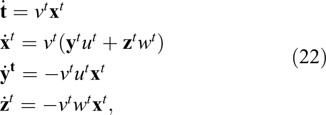
We control the leader utilizing the 3-D chasing controller in the study by Reddy et al. ¹¹ To simulate the target movement, we utilized Frenet–Serret frames ^11,31 as follows

$\begin{array}{l}\dot{\mathbf{t}}=v^t{\mathbf{x}}^t\\ {\dot{\mathbf{x}}}^t=v^t({\mathbf{y}}^t{u}^t+{\mathbf{z}}^t{w}^t)\\ {\dot{\mathbf{y}}}^{\mathbf{t}}=-v^t{u}^t{\mathbf{x}}^t\\ {\dot{\mathbf{z}}}^t=-v^t{w}^t{\mathbf{x}}^t,\end{array}$

22

where the natural curvatures u^t and w^t are target’s controllers. $v^{\mathbf{t}}$ is 0.5, which is slightly smaller than $v^{\mathbf{f}}=0.6$ . $\mathbf{t}$ is the target’s 3-D location. Note that $\{{\mathbf{x}}^t,{\mathbf{y}}^t,{\mathbf{z}}^t\}$ is natural Frenet frame (relatively parallel adapted frame) for the target’s trajectories. ¹¹

We give the target two behaviors: (1) if the target detects a follower, then the target moves in the opposite direction to avoid capture and (2) if the target detects no followers, then the target moves using its predefined $u^{\mathbf{t}}$ and $w^{\mathbf{t}}$ . Each simulation continues until the relative distance between the leader and the target is smaller than $2\times v^f$ distance units.

Noiseless simulations

$(x_k,y_k,z_k)-{\mathbf{t}}_k$ represents sensor noise and is a vector with three elements. In this subsection, we consider noiseless sensing. Thus, $(x_k,y_k,z_k)={\mathbf{t}}_k$ , and the target prediction is accurate, that is, ${\widehat{\mathbf{t}}}_{k+1}={\mathbf{t}}_{k+1}$ at each time step k.

Figure 7 shows how the system behaves when $u^{\mathbf{t}}$ and $w^{\mathbf{t}}$ in equation (22) are 0.01 and −0.01, respectively. Considering the scenario in Figure 7, Figure 8 presents S_s with respect to time index. S_s of each follower is negative initially, which implies that a follower is detected by the target initially. S_s of each follower becomes positive as time index increases. This indicates that every follower becomes unobservable as time index increases. Figure 8 further shows the distance between a follower and its closest robot with respect to time index. See that collision avoidance is assured for each robot under our controller.

Figure 7.

The robot and target trajectories ( $u^{\mathbf{t}}$ and $w^{\mathbf{t}}$ in equation (22) are 0.01 and −0.01, respectively).

Figure 8.

Left figure: unobservable state with respect to time index. Right figure: distance between a follower and its closest robot with respect to time index ( $u^{\mathbf{t}}$ and $w^{\mathbf{t}}$ in equation (22) are 0.01 and −0.01, respectively).

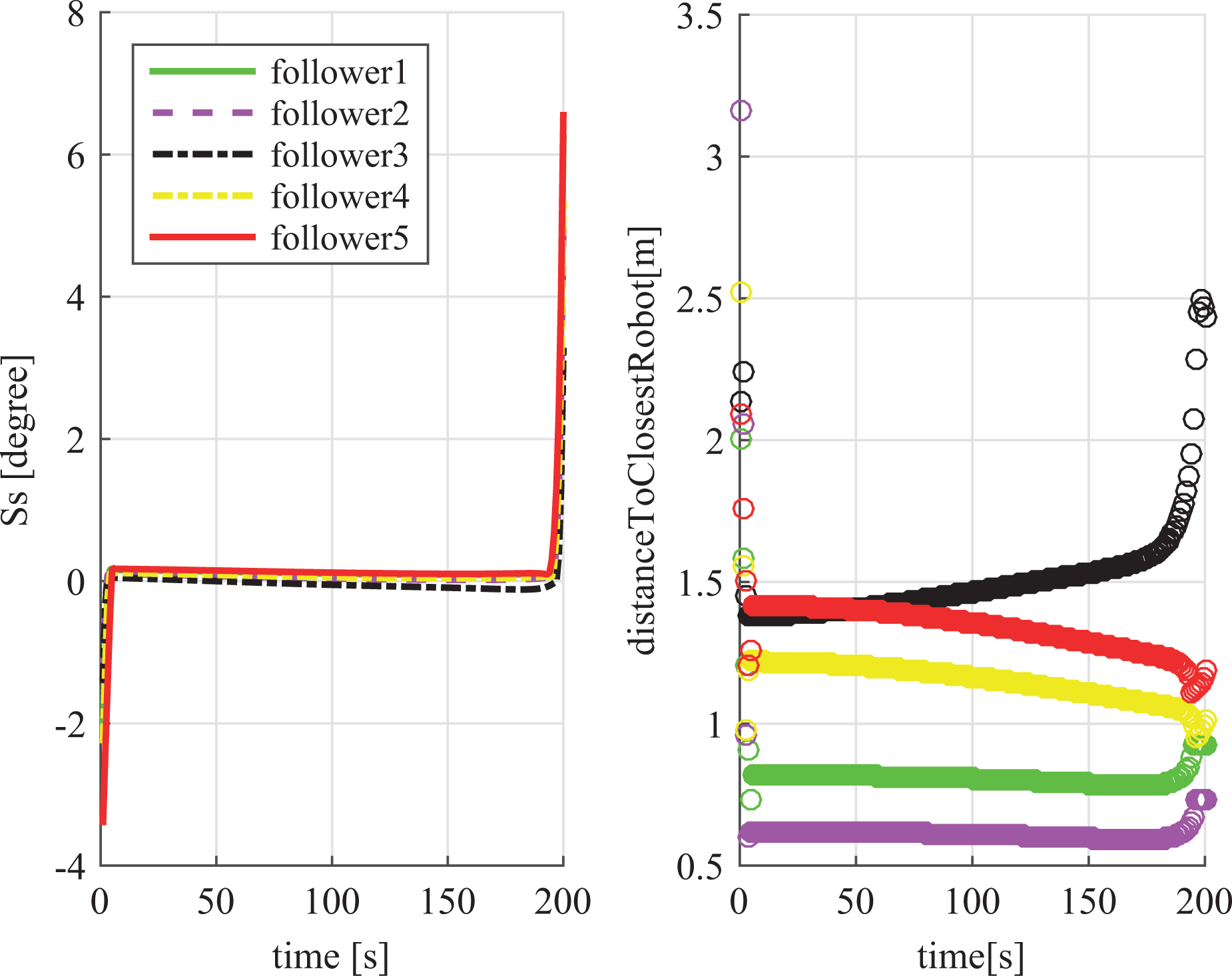
Figure 9 shows the system behavior when $u^{\mathbf{t}}$ and $w^{\mathbf{t}}$ in equation (22) are $0.05\text{sin}(\mathbf{t}/10)$ and −0.01, respectively. Considering the scenario in Figure 9, Figure 10 presents S_s with respect to time index. S_s of each follower becomes positive as time index increases. This indicates that every follower becomes unobservable as time index increases. Also, Figure 10 shows the distance between a follower and its closest robot with respect to time index. See that collision avoidance is assured for each robot under our controller.

Figure 9.

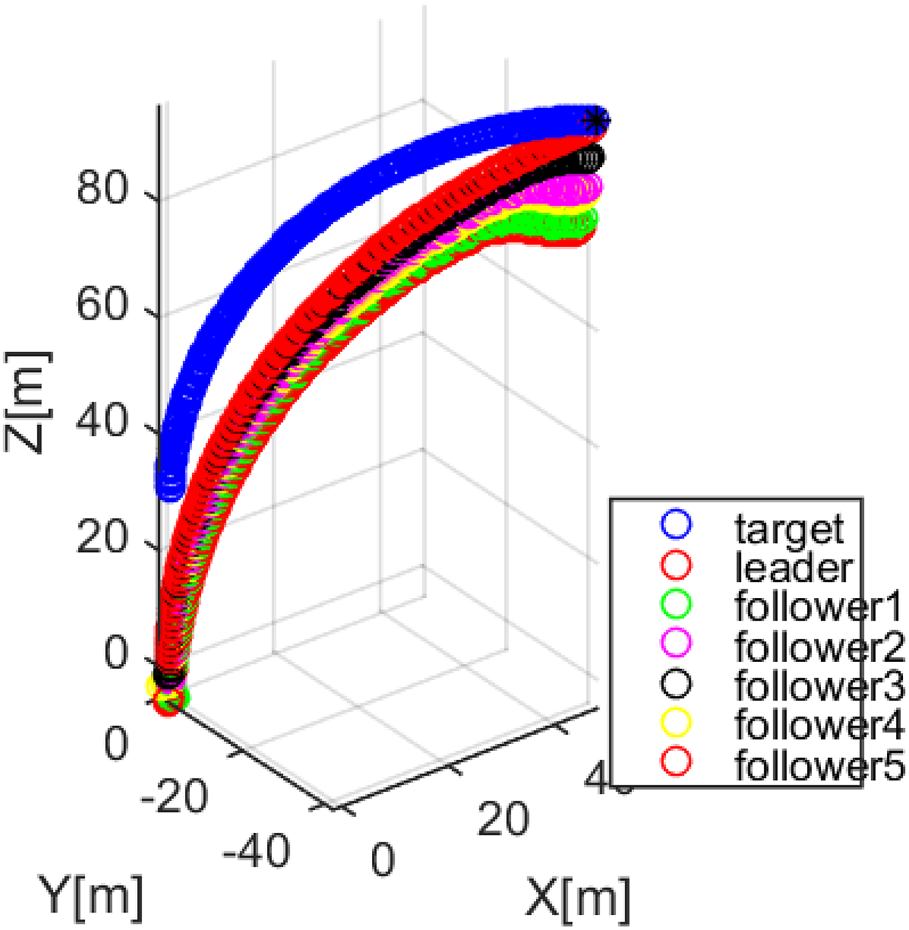
The robot and target trajectories ( $u^{\mathbf{t}}$ and $w^{\mathbf{t}}$ in equation (22) are $0.05\text{sin}(\mathbf{t}/10)$ and −0.01, respectively).

Figure 10.

Left figure: unobservable state with respect to time index. Right figure: distance between a follower and its closest robot with respect to time index ( $u^{\mathbf{t}}$ and $w^{\mathbf{t}}$ in equation (22) are $0.05\text{sin}(\mathbf{t}/10)$ and −0.01, respectively).

Theorem 4 proved that Fⁱ avoids colliding with F^m for every time index $k>k^{i,m}+1$ . Here, $k^{i,m}+1$ is a time index satisfying that both ${\mathbf{f}}_{k^{i,m}+1}^i$ and ${\mathbf{f}}_{k^{i,m}+1}^m$ are on $L_{k^{i,m}+1}$ . Theorem 4 proved that the relative distance between Fⁱ and F^m does not change for every time index $k>k^{i,m}+1$ . However, Figures 8 and 10 show that the distance between a follower and its closest robot slowly changes even after a follower is located on L. This is due to the fact that the bearing line of the leader, whose motion is controlled under the 3-D controller in the Reddy et al.’s study, ¹¹ rotates slowly.

Noisy simulations

In this subsection, we consider noisy environments. $(x_k,y_k,z_k)-{\mathbf{t}}_k$ represents sensor noise and is a vector with three elements. Each element in $(x_k,y_k,z_k)-{\mathbf{t}}_k$ has Gaussian distribution with mean 0 and covariance 0.1

Figure 11 shows how the system behaves when $u^{\mathbf{t}}$ and $w^{\mathbf{t}}$ in equation (22) are 0.01 and −0.01, respectively. Considering the scenario in Figure 11, Figure. 12 presents S_s with respect to time index. S_s of each follower is negative initially, which implies that a follower is detected by the target initially. In general, S_s of each follower becomes positive as time index increases. However, S_s becomes negative occasionally, due to noisy environments. Figure 12 further shows that collision avoidance is assured for each robot under our controller.

Figure 11.

The robot and target trajectories in noisy environments ( $u^{\mathbf{t}}$ and $w^{\mathbf{t}}$ in equation (22) are 0.01 and −0.01, respectively).

Figure 12.

Simulations in noisy environments. Left figure: unobservable state with respect to time index. Right figure: distance between a follower and its closest robot with respect to time index ( $u^{\mathbf{t}}$ and $w^{\mathbf{t}}$ in equation (22) are 0.01 and −0.01, respectively).

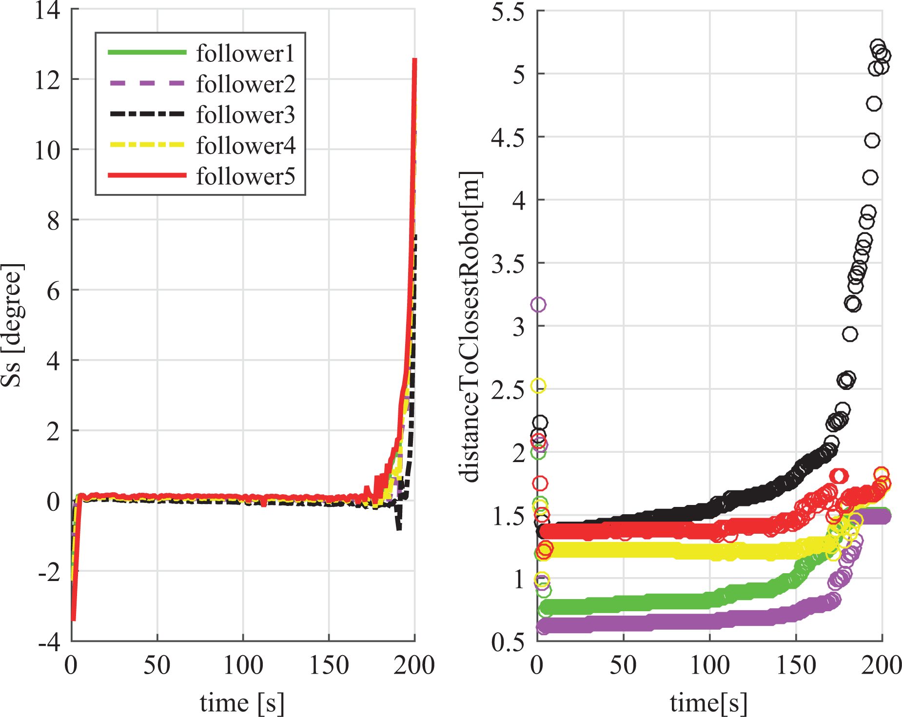
Figure 13 shows the system behavior when $u^{\mathbf{t}}$ and $w^{\mathbf{t}}$ in equation (22) are $0.05\text{sin}(\mathbf{t}/10)$ and −0.01, respectively. Considering the scenario in Figure 13, Figure 14 presents S_s with respect to time index. In general, S_s of each follower becomes positive as time index increases. However, S_s becomes negative occasionally, due to noisy environments. Also, Figure 14 shows that collision avoidance is assured for each robot under our controller.

Figure 13.

The robot and target trajectories in noisy environments ( $u^{\mathbf{t}}$ and $w^{\mathbf{t}}$ in equation (22) are $0.05\text{sin}(\mathbf{t}/10)$ and −0.01, respectively).

Figure 14.

Simulations in noisy environments. Left figure: unobservable state with respect to time index. Right figure: distance between a follower and its closest robot with respect to time index ( $u^{\mathbf{t}}$ and $w^{\mathbf{t}}$ in equation (22) are $0.05\text{sin}(\mathbf{t}/10)$ and −0.01, respectively).

Conclusions

This article introduces a 3-D multi-agent control which is to make a team of robots get closer to a target while not being observed by the target. Our 3-D chasing controller is to control followers so that they are not observed, blocked by the stealth leader. This article further proves that under our stealth control with some condition satisfied, multiple robots avoid colliding with each other. Simulations are utilized to demonstrate the effectiveness of our 3-D multi-agent controller.