Sage Journals: Discover world-class research

Abstract

To avoid the saturation of momentum wheels and the harm due to the thruster plume during the on-orbital manipulation, space robots usually stay in a free-floating state which follows the linear and angular momentum conservation leading to a kinematic coupling effect of the satellite base and the space manipulator. Emphasizing the stability of satellite base and execution safety, it is significant to minimize the kinematic coupling effect as well as avoid obstacles in the environment. Nevertheless, coupling minimization and obstacles avoidance are considered separately in previous work. By applying a hybrid map in the Configuration space, this article proposes a unified method dealing with the above two problems together. First, coupling factors are defined to evaluate the kinematic coupled effect which can be described by a coupling map; second, an obstruction map is generated by transforming obstacles in the Cartesian space to the Configuration space; the proposed hybrid map is finally generated from an overlay of a coupling map and an obstruction map. Numerical simulations verify the effectiveness of the method on a two degree-of-freedom planar space robot.

Keywords

Space robot coupling minimization obstacles avoidance hybrid map configuration space

Introduction

Unmanned orbital operation by space robots is a significant way to perform on-orbital service.¹ With the development of robotics, the manipulation of space robots continues to show great advantages and benefits in on-orbital servicing missions, including docking, berthing, refueling, repairing, upgrading, transporting, rescuing, and orbital debris removal.^2
–4 Because of the microgravity environment in space, the space robot is usually in a free-floating state to avoid the saturation of momentum wheels and the harm due to the thruster plume.^5,6 The dynamic coupling between the manipulator and the base makes it more difficult to control motion.^7,8 Besides, the space robot is facing the threat of obstacles such as space debris.⁹ To ensure the flight safety, the space robot needs to achieve autonomous obstacles avoidance with coupling minimization.^10,11

To solve the problem of coupling interference between the manipulator and the base, many researches have been carried out by utilizing the nonholonomic properties of the space robot system.¹² Inspired by astronauts to adjust body balance by moving their extremities, Vafa and Dubowsky¹³ introduced an approach called Virtual Manipulator to simplify the kinematics and analyze the workspace of a space robot. They proposed a self-correcting motion method that used the cyclic motion of the robot’s joint to change the attitude of the base. Umetani and Yoshida¹⁴ defined the Generalized Jacobian Matrix (GJM) to replace the traditional Jacobian matrix, which enabled the fixed-base approach to be extended to free-floating space robots. Based on the GJM, Xu et al.^15,16 presented the coupling factor to measure the degrees of dynamic coupling between the manipulator and the base. Xu et al.¹⁷ used hybrid dynamic coupling modeling and analysis methods to solve the problem of various singular configurations and low computational efficiency. However, these methods didn’t consider obstacles avoidance as well. To achieve obstacles avoidance for space robot, Lozano-Perez et al.¹⁸ proposed a free space method in the Configuration space. The Configuration space was established by the joint coordinate system of the manipulator, and the heuristic search algorithm was used to search the path of the manipulator in the free space. Wang et al.¹⁹ regarded obstacles avoidance as a constraint of motion control and used the online quadratic programming program to obtain the constrained optimal control in real time. Liu et al.²⁰ proposed an approach about obstacle collision-free motion planning of space manipulator by utilizing a Configuration-Oriented Artificial Potential Field method. Zhou et al²¹ proposed an improved ant colony algorithm to avoid obstacles. The method was effective and simple, but it didn’t consider the coupling disturbance. In general, in the process of path planning, it is difficult to consider coupling minimization and obstacle avoidance together.

In this article, we present a hybrid method in the Configuration space to achieve both coupling minimization and obstacles avoidance of free-floating space robots, by unifying the coupling map and the obstruction map to the hybrid map. First of all, this article analyzes the kinematic coupling effect between the manipulator and the base by kinematics modeling, establishing a coupling map to describe quantitatively. Secondly, an obstruction map is generated by converting obstacles from the Cartesian space into the Configuration space by the theory of the Configuration space. Finally, the coupling map is superimposed with the obstruction map to construct a hybrid map in the Configuration space.

The remainder of this article is arranged as follows. In second section, we derive the kinematic equations and the momentum conservation equations for space robots and establish the theoretical basis of the coupling map. In this section, we first introduce the generation and function of the coupling map. Then, we introduce the theory of the Configuration space and establish the obstruction map in the Configuration space. Finally, we put forward the concept of the hybrid map in the Configuration space and present the quantitative criterion of the hybrid map. Simulation experiment of path planning is conducted to verify the effectiveness of the proposed method in the fourth section. In the final section, we offer a conclusion of the study.

Kinematic modeling and coupling effect analysis

A space robot can be described as a tree-shaped multi-rigid-body system in which the head and the end are connected with each other. The position, attitude, and the joint angles are often chosen as the generalized coordinates to describe the motion of the space robot, which form the Configuration space of the space robot. When using space robots to perform space missions, people are generally concerned about the trajectory of the end-effector in the Cartesian space. One is to require that the path of end effector satisfies certain constraints in the Cartesian space.^22,23 The other is to achieve accurate tracking of the desired path.^24,25 In this section, the robot kinematics is modeled to solve the mathematical expression of the relationship between the generalized coordinates of the space robot and the trajectory of the end-effector. Besides, the conversion of space robots is established from the Cartesian space to the Configuration space. Since the kinematics modeling theory is very mature, the explanation process in this section omits some unnecessary details.

Kinematic modeling

As shown in Figure 1, the space robot is described as a tree-shaped multi-body system in this section. According to the research method proposed by Xu,¹⁵ the generalized velocity of the end-effector can be obtained as

[\begin{array}{l} v_{e}^{k} \\ ω_{e}^{k} \end{array}] = J_{b}^{k} [\begin{array}{l} v_{0} \\ ω_{0} \end{array}] + J_{m}^{k} \dot{θ}

where $J_{b}^{k}$ is the Jacobian matrix associated with the motion of the base, and $J_{m}^{k}$ is the Jacobian matrix associated with the motion of the manipulator. Their detailed definitions are as follows

J_{b}^{k} = (\begin{array}{l} E_{3} - {\tilde{p}}_{0 e}^{k} \\ O E_{3} \end{array}) = [\begin{array}{l} J_{b v}^{k} \\ J_{b w}^{k} \end{array}] \in R^{6 \times 6}

{\tilde{p}}_{0 e}^{k} = p_{e}^{k} - r_{0}

J_{m}^{k} = [\begin{array}{l} k_{1}^{k} \times (p_{e}^{k} - p_{1}^{k}) \cdot \cdot \cdot k_{n}^{k} \times (p_{e}^{k} - p_{n}^{k}) \\ k_{1}^{k} \cdot \cdot \cdot k_{n}^{k} \end{array}] = [\begin{array}{l} J_{m v}^{k} \\ J_{m w}^{k} \end{array}] \in R^{6 \times n}

where $J_{b v}^{k}$ and $J_{b w}^{k}$ are block matrixes associated with linear velocity and angular velocity. $J_{m v}^{k}$ and $J_{m w}^{k}$ are block matrixes of $J_{m}^{k}$ .

Figure 1.

The tree-shaped system of a space robot.

The initial linear momentum and angular momentum of the system is defined $P_{0}$ and $L_{0}$ , respectively. According to the conservation of linear momentum and angular momentum, we can obtain

P = m_{0} v_{0} + \sum_{k = 1}^{N} (\sum_{i = 1}^{n_{k}} m_{i}^{k} {\dot{r}}_{i}^{k}) = P_{0}

L = (I_{0} ω_{0} + r_{0} \times m_{0} {\dot{r}}_{0}) + \sum_{k = 1}^{2} (\sum_{i = 1}^{n_{k}} (I_{i}^{k} ω_{i}^{k} + r_{i}^{k} \times m_{i}^{k} {\dot{r}}_{i}^{k})) = L_{0}

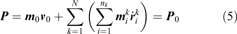
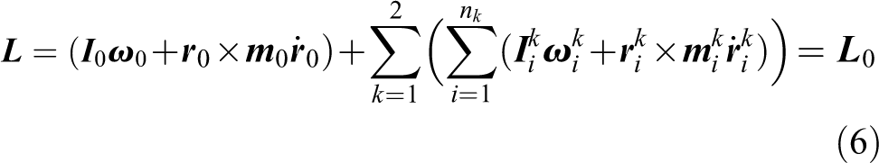
For the convenience of subsequent discussions, the above two formulas are further written as

[\begin{array}{l} P \\ L \end{array}] = (\begin{matrix} ME & M {\tilde{r}}_{o g}^{T} \\ M {\tilde{r}}_{g} & I_{w} \end{matrix}) [\begin{array}{l} v_{0} \\ ω_{0} \end{array}] + \sum_{k = 1}^{N} ([\begin{array}{l} J_{T w}^{k} \\ I_{ϕ}^{k} \end{array}] {\dot{q}}_{k}) = [\begin{array}{l} P_{0} \\ L_{0} \end{array}]

where

I_{w} = I_{0} + \sum_{k = 1}^{N} (\sum_{i = 1}^{n_{k}} (I_{i}^{k} + m_{i}^{k} {\tilde{r}}_{i}^{k} {({\tilde{r}}_{0 i}^{k})}^{T}))

I_{ϕ}^{k} = \sum_{i = 1}^{n_{k}} (I_{i}^{k} J_{R i}^{k} + m_{i}^{k} {\tilde{r}}_{i}^{k} J_{T i}^{k})

r_{0 g} = r_{g} - r_{0}

r_{0 i}^{k} = r_{i}^{k} - r_{0}

J_{T w}^{k} = \sum_{i = 1}^{n_{k}} (m_{k}^{i} J_{T i}^{k}) \in R^{3 \times n_{k}}

J_{T i}^{k} = {\begin{matrix} [z_{1}^{k} \times (r_{i}^{k} - p_{1}^{k}) \cdot \cdot \cdot z_{i}^{k} \times (r_{i}^{k} - p_{i}^{k}) 0 \cdot \cdot \cdot 0] \in R^{3 \times n_{k}}, Rotating joint \\ [z_{1}^{k} \cdot \cdot \cdot z_{i}^{k} 0 \cdot \cdot \cdot 0] \in R^{3 \times n_{k}}, Prismatic joint \end{matrix}

J_{R i}^{k} = {\begin{cases} [z_{1}^{k} \cdot \cdot \cdot z_{i}^{k} 0 \cdot \cdot \cdot 0] \in R^{3 \times n_{k}}, Rotating joint \\ [0 \cdot \cdot \cdot 00 \cdot \cdot \cdot 0] \in R^{3 \times n_{k}}, Prismatic joint \end{cases}

Equation (7) can be reduced as follows:

H_{b} {\dot{x}}_{0} + \sum_{k = 1}^{N} (H_{b m}^{k} {\dot{q}}^{k}) = M_{0}

where

H_{b} = (\begin{matrix} ME & M {\tilde{r}}_{o g}^{T} \\ M {\tilde{r}}_{g} & H_{w} \end{matrix}) \in R^{6 \times 6}

H_{b m}^{k} = [\begin{array}{l} J_{T w}^{k} \\ I_{ϕ}^{k} \end{array}] \in R^{6 \times n_{k}}

M_{0} = [\begin{array}{l} P_{0} \\ L_{0} \end{array}] \in R^{6 \times 1}

According to equation (15), we establish a kinematic model of a free-floating space robot based on the GJM. Further, based on the theorems of linear momentum and angular momentum conservation, the coupling matrix between the generalized coordinates of the manipulator and the base is deduced. Through the coupling matrix, the motion state of base can be determined by the motion state of the manipulator. Further, the degree of the kinematic coupling effect can be measured to guide the path planning of the space robot.

Coupling factor

Since the free-floating space robot satisfies the conservation of linear momentum and angular momentum, we can define the initial linear momentum and angular momentum to be zero. The mass center of the space robot system is still in inertial space. From the derivation of equation (15), we can get the following equation

H_{b} {\dot{x}}_{0} + \sum_{k = 1}^{N} (H_{b m}^{k} {\dot{q}}^{k}) = 0

ω_{0} = - H_{s}^{- 1} H_{θ} \dot{θ}

v_{0} = ({\tilde{p}}_{e}^{x} ω_{0} - {\tilde{J}}_{m v} \dot{θ}) = (- {\tilde{p}}_{e}^{x} H_{s}^{- 1} H_{θ} - {\tilde{J}}_{m v}) \dot{θ}

where

H_{s} = M r_{g}^{x} {\tilde{p}}_{e}^{x} + I_{w}

H_{θ} = I_{ϕ} - M r_{g}^{x} {\tilde{J}}_{m v}

{\tilde{J}}_{m v} = [\begin{matrix} k_{1} \times ({\tilde{p}}_{e} - {\tilde{p}}_{1}) & \dots & k_{n} \times ({\tilde{p}}_{e} - {\tilde{p}}_{n}) \end{matrix}]

The joint-base translational coupling matrix $C_{b j}^{r} \in R^{3 \times n}$ and the joint-base rotational coupling matrix $C_{b j}^{w} \in R^{3 \times n}$ are defined as follows

C_{b j}^{r} = = - {\tilde{p}}_{e}^{x} H_{s}^{- 1} H_{θ} - {\tilde{J}}_{m v}

C_{b j}^{w} = - H_{s}^{- 1} H_{θ}

Then, according to the equations (20) and (21), we can get the result as follows

v_{0} = (- {\tilde{p}}_{e}^{x} H_{s}^{- 1} H_{θ} - {\tilde{J}}_{m v}) \dot{θ} = C_{b j}^{r} \dot{θ}

ω_{0} = - H_{s}^{- 1} H_{θ} \dot{θ} = C_{b j}^{w} \dot{θ}

Equations (27) and (28) can be combined into the following format

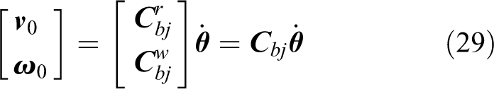
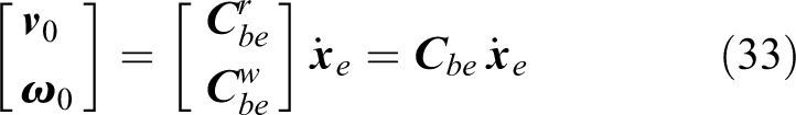
[\begin{array}{l} v_{0} \\ ω_{0} \end{array}] = [\begin{array}{l} C_{b j}^{r} \\ C_{b j}^{w} \end{array}] \dot{θ} = C_{b j} \dot{θ}

Substituting equation (29) into equation (1), the following equation is obtained

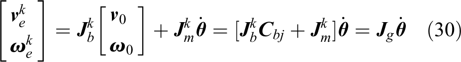
[\begin{array}{l} v_{e}^{k} \\ ω_{e}^{k} \end{array}] = J_{b}^{k} [\begin{array}{l} v_{0} \\ ω_{0} \end{array}] + J_{m}^{k} \dot{θ} = [J_{b}^{k} C_{b j} + J_{m}^{k}] \dot{θ} = J_{g} \dot{θ}

where $J_{g} = J_{b}^{k} C_{b j} + J_{m}^{k}$ is known as the GJM.

Substituting equation (30) into equations (27) and (28), the following equation is obtained

v_{0} = C_{b j}^{r} \dot{θ} = C_{b j}^{r} J_{g}^{- 1} {\dot{x}}_{e} = C_{b e}^{r} {\dot{x}}_{e}

ω_{0} = C_{b j}^{w} \dot{θ} = C_{b j}^{w} J_{g}^{- 1} {\dot{x}}_{e} = C_{b e}^{w} {\dot{x}}_{e}

where $C_{b e}^{r} = C_{b j}^{r} J_{g}^{- 1} \in R^{3 \times 6}$ and $C_{b e}^{w} = C_{b j}^{w} J_{g}^{- 1} \in R^{3 \times 3}$ are the end-base translational coupling matrix and the end-base rotational coupling matrix. Equations (31) and (32) can be combined into the following format

[\begin{array}{l} v_{0} \\ ω_{0} \end{array}] = [\begin{array}{l} C_{b e}^{r} \\ C_{b e}^{w} \end{array}] {\dot{x}}_{e} = C_{b e} {\dot{x}}_{e}

Coupling factors $w_{b j}^{r} (\dot{θ})$ , $w_{b j}^{ω} (\dot{θ})$ , $w_{b e}^{r} ({\dot{x}}_{e})$ , and $w_{b e}^{ω} ({\dot{x}}_{e})$ are defined as follows

w_{b j}^{r} (\dot{θ}) = \frac{{‖ v_{0} ‖}_{2}}{{‖ \dot{θ} ‖}_{2}} = \sqrt{\frac{{\dot{θ}}^{T} ({(C_{b j}^{r})}^{T} C_{b j}^{r}) \dot{θ}}{{\dot{θ}}^{T} \dot{θ}}} = \sqrt{\frac{{\dot{θ}}^{T} A_{b j}^{r} \dot{θ}}{{\dot{θ}}^{T} \dot{θ}}}

w_{b j}^{ω} (\dot{θ}) = \frac{{‖ ω_{0} ‖}_{2}}{{‖ \dot{θ} ‖}_{2}} = \sqrt{\frac{{\dot{θ}}^{T} ({(C_{b j}^{ω})}^{T} C_{b j}^{ω}) \dot{θ}}{{\dot{θ}}^{T} \dot{θ}}} = \sqrt{\frac{{\dot{θ}}^{T} A_{b j}^{ω} \dot{θ}}{{\dot{θ}}^{T} \dot{θ}}}

w_{b e}^{ω} ({\dot{x}}_{e}) = \frac{{‖ ω_{0} ‖}_{2}}{{‖ {\dot{x}}_{e} ‖}_{2}} = \sqrt{\frac{{\dot{x}}_{e} ​^{T} ({(C_{b e}^{ω})}^{T} C_{b e}^{ω}) {\dot{x}}_{e}}{{\dot{x}}_{e} ​^{T} {\dot{x}}_{e}}} = \sqrt{\frac{{\dot{x}}_{e} ​^{T} A_{b e}^{ω} {\dot{x}}_{e}}{{\dot{x}}_{e} ​^{T} {\dot{x}}_{e}}}

w_{b e}^{r} ({\dot{x}}_{e}) = \frac{{‖ ω_{0} ‖}_{2}}{{‖ {\dot{x}}_{e} ‖}_{2}} = \sqrt{\frac{{\dot{x}}_{e} ​^{T} ({(C_{b e}^{r})}^{T} C_{b e}^{r}) {\dot{x}}_{e}}{{\dot{x}}_{e} ​^{T} {\dot{x}}_{e}}} = \sqrt{\frac{{\dot{x}}_{e} ​^{T} A_{b e}^{r} {\dot{x}}_{e}}{{\dot{x}}_{e} ​^{T} {\dot{x}}_{e}}}

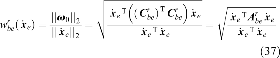
In equation (35), $w_{b j}^{ω} (\dot{θ})$ describes the attitude change of the base for a given motion of joints. $A_{b j}^{w}$ is a n-order real symmetric square and the eigenvalues of the matrix $A_{b j}^{w}$ are the spectral values of the coupling matrix $C_{b j}^{w}$ . We assuming that $λ_{min} (A_{bj}^{ω})$ is the minimum eigenvalue of the matrix $A_{b j}^{w}$ , and the maximum is $λ_{max} (A_{bj}^{ω})$ . According to measure method proposed in,¹⁵ we can get the following equation

\sqrt{λ_{min} (A_{bj}^{ω})} \leq w_{b j}^{ω} (\dot{θ}) \leq \sqrt{λ_{max} (A_{bj}^{ω})}

From equation (38), the range of the kinematic coupling effect between the motion of manipulator and the attitude of base is defined. Based on the same theory, the value range of the other three coupling factors can also be discussed.

According to equations (34) to (38), coupling factors are determined by geometry structure and motion state of the space robot. Once the geometry structure is determined, coupling factors are only functions of the motion state. At the same time, the motion state of the space robot can be expressed as a function of generalized coordinates, which are functions of the joint angle. Therefore, once the geometry structure of the space robot is determined, coupling factors are only functions of the joint angle.

Hybrid map in the configuration space

To comprehensively consider coupling minimization and obstacles avoidance in the Configuration space, we first map the information in the Cartesian space to the Configuration space. This information consists of two parts, one is the coupling factor, and the other is the robotic configuration and the obstacle position. In this section, we first introduce the coupling map formed by the coupling factor in the Configuration space. Then, we introduced the generation method of the obstruction map. Finally, we introduce the theoretical basis and generation method of the hybrid maps in the Configuration space.

Coupling map in the configuration space

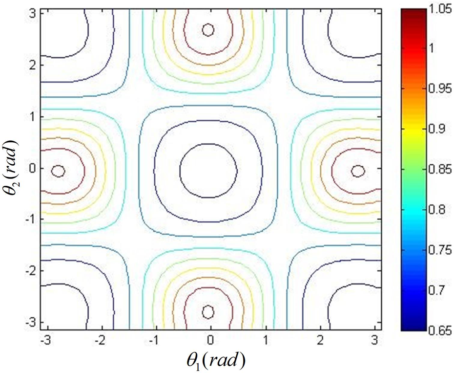
To express the change of the coupling factor more intuitively, we draw an n-dimensional map of its values. We define the n-dimensional map of the coupling factor as a coupling map. The size of n is determined by the dimensions of generalized coordinate of space robots. In the tree-shaped multi-body system of space robots, the size of n is equal to the number of joint angles. Each dimensional space represents a joint angle. We define the value of the coupling factor as the altitude of the coupling map. The boundary of the altitude is determined by equation (38).

According to the formulas (34) to (37), the 3-D curve of each coupling factor can be obtained when the joint angle changes from 0° to 360°. As shown in Figure 2, a coupling map of a two-joint robot is drawn. Since the path planning is performed in the two-dimensional space, this article projects the 3-D curve onto the two-dimensional plane, which is shown in Figure 3. By further analysis, a contour of the coupling factor as a function of joint angle can be obtained, as shown in Figure 4.

Figure 2.

The coupling map of a two-joint robot.

Figure 3.

The projection of coupling map.

Figure 4.

The contour of coupling map.

As shown in Figure 3, the red area is called “Hot Zone,” where the disturbance between the manipulator and the base is large. And the blue area is called “Cold Zone,” where the disturbance is small. During the movement of the robot, it is necessary to avoid disturbing ‘Hot Zone’. Besides, the disturbance of each point can be quantitatively described by the contour lines divided in Figure 4, which can be used as a basis for motion planning.

Obstruction map in the configuration space

It is straightforward and convenient to avoid obstacles for space robots in the Cartesian space, but it is very difficult to ensure that all points on the robot can avoid obstacles. In addition, the planned trajectories for obstacles avoidance in the Cartesian space may not be able to avoid all the singularities of space robots and even require infinite velocities of robotic joints. Further, most of space robots are controlled by its joints. The conversion of planned trajectories is complex from the Cartesian space to the Configuration space, which makes it difficult to achieve real-time control of space robots. To solve the above problems, many researchers have proposed to employ the Configuration space theory into the path planning of space robots.^26,27 First, space robots and obstacles are converted into the Configuration space to generate the planning map. Then, based on the planning map, the path planning strategy is used to search for the optimal path.

For the convenience of the following description, the specific definitions are given as follows:

Q: the space robot in the Cartesian space;

$U = {U_{1}, U_{2} \dots U_{n}}$ : information collection of obstacles, where $U_{i}$ represents the information of ith obstacle;

$C (Q, U)$ : the Configuration space;

C_Q : the Configuration space of space robots;

$C_{obstacle} (Q, U) = {C_{obstacle} (Q, U_{1}) \dots C_{obstacle} (Q, U_{n})}$ : the obstacle space, where $C_{obstacle} (Q, U_{i})$ represents the obstacle space corresponding to ith obstacle; and

$C_{free} (Q, U)$ : the free space.

The Configuration space is also known as the Joint space or C-space. Its main idea is a conversion from the Cartesian space to the Configuration space. Firstly, space robots and obstacles are converted to form the Configuration space $C (Q, U)$ . Then, the Configuration space is divided into two subspaces, the obstacle space $C_{o b s t a c l e} (Q, U)$ and the free space $C_{f r e e} (Q, U)$ . The specific definitions are as follows

C_{obstacle} (Q, U) = {c \in C (Q, U) | R (c) \cap U \neq \emptyset}

C_{free} (Q, U) = C (Q, U) \ C_{obstacle} (Q, U)

where $R (\cdot)$ represents the solution process of forward kinematics. It maps the configuration space area to Cartesian space.

After the analysis in second section, we can conclude that the pose of the space robot is determined by its generalized coordinates. And the generalized coordinates are a function of the joint angle $θ = {[θ_{1}, θ_{2} \dots θ_{n}]}^{T}$ . Therefore, the pose of space robot can be expressed as a point C_Q in the configuration space. On the other hand, the pose in which the space robot collides with obstacles constitutes the obstacle space. Therefore, the pose of the space robot and the point in the Configuration space are one-to-one correspondence. To visually describe the distribution of obstacles in the Configuration space, we draw a map of the obstacles space named the obstruction map.

As shown in Figure 5, the left is a planar two degree-of-freedom robot with fixed base in the Cartesian space. The start pose of the robot is shown in the left figure and the black rectangle is an obstacle. This article defines the start point of path planning as A and the end point as B. The right is the Configuration space corresponding to the left. The abscissa corresponds to the first joint angle of the manipulator named α, whose range is from 0 to π. And the ordinate corresponds to the second joint angle of the manipulator named β, whose range is from 0 to 2π. The point C_A corresponds to the initial state of the robot and the point C_B corresponds to the final state of the robot. The black area is the obstacle space $C_{obstacle} (Q, U)$ , and the rest is the free space $C_{free} (Q, U)$ . We find that there is not a connecting path between points C_A and C_B in the Configuration space. Therefore, we conclude that the start point A cannot be moved to the end point B in the Cartesian space due to the blockage of the obstacle.

Figure 5.

The conversion between the Cartesian space and the configuration space.

The space robot can capture images in the Cartesian space by its global camera and the obstacle information can be easily obtained by the recognition algorithm. Therefore, the obstacle information is regarded as known information in the article. To reduce the computation times and improve the efficiency of generating obstruction map, this article uses the idea of grid method to divide the Configuration space into m × n small squares. As shown in Figure 6, the length and width of small squares are w and h, where $w = 2 π / m, h = 2 π / n$ . $C_{i, j} (1 \leq i \leq n, 1 \leq j \leq m)$ represents the ith row and the jth column of small squares.

Figure 6.

The correspondence between grid coordinates and serial numbers.

For all the squares $C_{i, j}$ in the Configuration space, we need to examine the collision between the space robot and the obstacles in the Cartesian space. When a collision occurs, the square is blacked out. When all the squares are tested, the union of all the black squares forms the obstacle subspace $C_{obstacle} (Q, U)$ in the Configuration space. Correspondingly, all the uncolored squares form the free subspace $C_{free} (Q, U)$ in the Configuration space. Collision detection between the areas swept by the space robot and the obstacles can be transformed into the collision detection between the convex polygons. There are many mature algorithms which will not be introduced here.

Hybrid map in the Configuration space

After the above analysis, we can conclude that both the coupling map and the obstruction map are functions of the joint angles $θ = {[θ_{1}, θ_{2} \dots θ_{n}]}^{T}$ . Therefore, this article defines the numerical coupling map as $CM = f (θ) = f (θ_{1}, θ_{2} \dots θ_{n})$ , and the numerical obstruction map as $O M = g (θ) = g (θ_{1}, θ_{2} \dots θ_{n})$ . The specific formulas for the coupling map and the obstruction map are as follows

f (θ) = w_{b j}^{ω} (\dot{θ}) o r w_{b j}^{ω} (\dot{θ}) o r w_{b e}^{r} ({\dot{x}}_{e}) o r w_{b e}^{ω} ({\dot{x}}_{e})

g (θ) = {\begin{cases} - \sum_{i = 1}^{k} min ‖ θ - C_{obstacle} (Q, U_{i}) ‖, θ \in C_{free} (Q, U) \\ - \infty, θ \in C_{obstacle} (Q, U) \end{cases}

where $min ‖ θ - C_{obstacle} (Q, U_{i}) ‖$ is minimum distance between point $θ = {[θ_{1}, θ_{2} \dots θ_{n}]}^{T}$ and ith obstacle.

To comprehensively consider the kinematic coupling effect and obstacles avoidance, this article superimposes two maps to construct a hybrid map in the configuration space. However, the two map functions have different measures. To make the two functions have the same metric, this article normalizes the two functions separately. After the above processing, the hybrid map is still a function of the joint angles $θ = {[θ_{1}, θ_{2} \dots θ_{n}]}^{T}$ , which is defined as $HMCS = h (θ) = h (θ_{1}, θ_{2} \dots θ_{n}) = α_{1} f (θ) + α_{2} g (θ)$ . Among them, α₁ and α₂ are the normalization coefficients of the two map functions, respectively. The specific process of the method is shown in Figure 7.

Figure 7.

The flow chart of hybrid map in the configuration space.

First of all, using the GJM, we set up the kinematics model of the space robot system and get the mathematical equations that describe the kinematics parameters of the robot. Then, based on the law of linear momentum and angular momentum conservation, we derive the coupling matrix between the generalized coordinates of the base and the space robot. Further, the range of the coupling factor is determined by the spectral radius of the coupling matrix. Finally, the article draws the coupling map in the Configuration space.

On the other hand, with the global camera carried by the space robot system, we can get the global map in the Cartesian space. Using well-established recognition algorithms, we can get location information of obstacles on the global map. In order to improve the efficiency of computing, we use the grid method to divide obstacles into small areas. By sampling in a small area and using the kinematics model established in “Obstruction map in the Configuration space” section, we obtain the obstacle space and the free space. Finally, the coupling map and the obstruction map are superposed, and the hybrid map in the Configuration space can be obtained.

Simulation experiment

In order to verify the feasibility and effectiveness of the proposed approach in this article, a simulation experiment is performed under the Windows 10 operating system. The processor model is Intel I5 7500 clocked at 3.4 GHz, and the graphics card is GTX 1070 (GPU). This article uses MATLAB 2013a to build a simulation system of the free-floating space robot. The two degree-of-freedom planar space robot is selected as the research object to carry out the simulation experiment. As shown in Figure 8, the base has two translational and one rotational degree-of-freedom, and the space manipulator has two rotating joints. The configuration parameters of the space robot are shown in Table 1.

Figure 8.

The two degree-of-freedom planar space robot.

Table 1.

Configuration parameters of the space robot.

B_i	m_i (kg)	a_i (m)	b_i (m)	I_i (kg m²)
B⁰	300	0	1.0	50
B¹	30	1.0	1.0	8
B²	30	1.0	1.0	8

Generation of the hybrid map

Generation of the coupling map

According to the theory described in “Coupling map in the Configuration space” section, configuration parameters of the space robot are shown in Table 1. When the end loads are m_L = 0 kg and m_L = 50 kg, respectively, the range of coupling factors is shown in Figure 9. The red curve indicates a unit circle, which means that the space manipulator and the base have the same kinematic coupling effect with each other. $λ_{min} (A_{b j}^{ω})$ is the semi-minor axis of the ellipse, and $λ_{max} (A_{b j}^{ω})$ is the semi-major axis of the ellipse. Table 2 shows the size of $λ_{min} (A_{b j}^{ω})$ and $λ_{max} (A_{b j}^{ω})$ when m_L = 0 kg, 50 kg, 100 kg, 150 kg, 200 kg, and 250 kg. From Figure 9 and Table 2, we can see that as the load increases, the kinematic coupling effect between the manipulator and the base gradually increases. This is in line with the conclusion we had before. Similarly, we can analyze the changes of other coupling factors under different loads.

Figure 9.

The size of coupling factor.

Table 2.

The size of coupling factor under different loads.

m_L (kg)	0	50	100	150	200	250
$λ_{min} (A_{b j}^{ω})$	0.0584	0.1278	0.1774	0.2137	0.2408	0.2617
$λ_{max} (A_{b j}^{ω})$	0.7805	0.8560	0.8999	0.9366	0.9692	0.9985

To express the change of the coupling factor in the whole process more clearly, this article further analyzes the size of the coupling factor under different angles. Taking the coupling factor $w_{b j}^{ω} (\dot{θ})$ as an example, the coupling map in 3-D form is shown in Figure 10. Since the simulation object selected in this article is a two-link space robot, the dimension of the coupling map is three. For the convenience of subsequent processing, we project the three-dimensional image onto the two-dimensional plane and draw the contour map of the coupling map shown in Figure 11. The larger coupling factor represented by the red contour area indicates that the robotic arm has a large disturbance to the base. On the other hand, the smaller coupling factor represented by the blue contour area indicates that the disturbance between the manipulator and the base is small.

Figure 10.

The coupling map in 3-D form.

Figure 11.

The contour of the coupling map.

Generation of the obstruction map

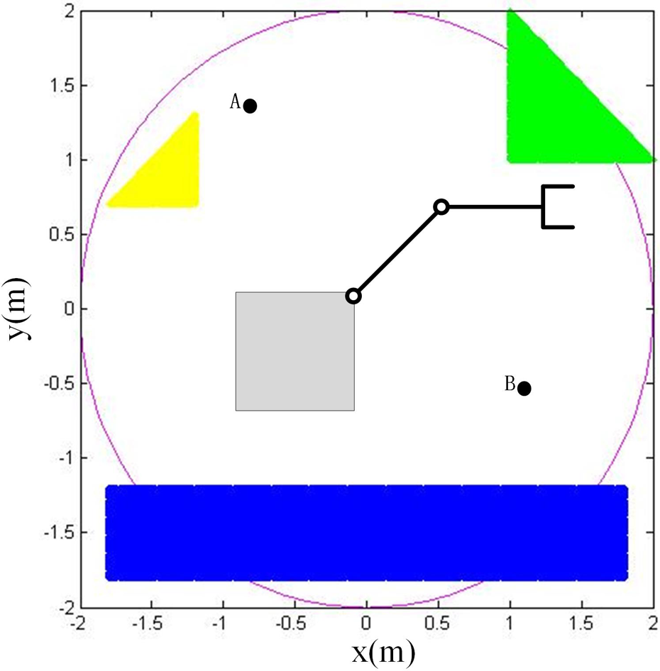
The distribution of obstacles in the Cartesian space is shown in Figure 12. The upper left yellow area is a right-angled triangle of size 0.6 × 0.6 m², the upper right green area is a right-angled triangle of size $1.0 \times 1.0 m^{2}$ , and the lower blue area is a rectangle of size $3.6 \times 0.5 m^{2}$ . In the follow-up simulation experiment, we assume that θ₁ and θ₂ are in the range of $[- π, + π]$ . The purple circle represents the maximum motion range of the robotic end-effector. When generating the obstruction space, we only do collision detection for areas within the purple circle.

Figure 12.

The obstruction distribution in the Cartesian space.

We use the method proposed in “Obstruction map in the Configuration space” section to convert obstacles in the Cartesian space to the Configuration space. In the process of actual programming, we choose 0.01 radian as the criterion of interval division and select nine pixels around the center as sampling points in each small square. Figure 13 is the obstruction map in the Configuration space converted from the Cartesian space. By observing the figure, we can get the following conclusions:

Due to the multi-solution characteristics of robotic inverse kinematics, a closed area in the Cartesian space corresponds to n closed areas in the Configuration space. The size of n is determined by the number of inverse solutions, and the closed areas can be connected together. Since the simulation object selected in this article is a two-link space robot, n is equal to two.

Due to the restrictions of sampling, the converted obstruction map is not a continuous closed area. When performing collision detection for path planning later, this article will take this effect into account.

The Configuration space is a continuous m-dimensional space graph, and the value of m is determined by the dimensions of robot’s generalized coordinate. In particular, the yellow obstacle is converted to three parts in the Configuration space. In fact, the two blocks on the left and right borders should be connected together by themselves. In order to show intuitively on a two-dimensional plane, we artificially divided it into two parts.

Figure 13.

Obstruction map in the configuration space.

Generation of the hybrid map

To consider the kinematic coupling effect and the obstacles avoidance together, the coupling map and the obstruction map are superposed to the hybrid map in the Configuration space, which is shown in Figure 14. In the hybrid map, every point contains both obstacle information and coupling information. At the same time, this article carries on the comprehensive operation of $f (θ)$ and $g (θ)$ to get the numerical characteristics of each point.

Figure 14.

Hybrid map in the configuration space.

As shown in Figure 14, each point in the Configuration space can be represented as a function of joint angle $θ = (θ_{1}, θ_{2} \dots θ_{n})$ . The state of the space robot at each moment corresponds to a point on Figure 14. The hybrid map in the Configuration space describes the positional relationship between the robot system and the obstacle at that moment and the internal coupling disturbance. Therefore, when designing the algorithm of path planning, the influence of the above two constraints can be conveniently measured.

Experiment of path planning

Evaluation criteria of path planning

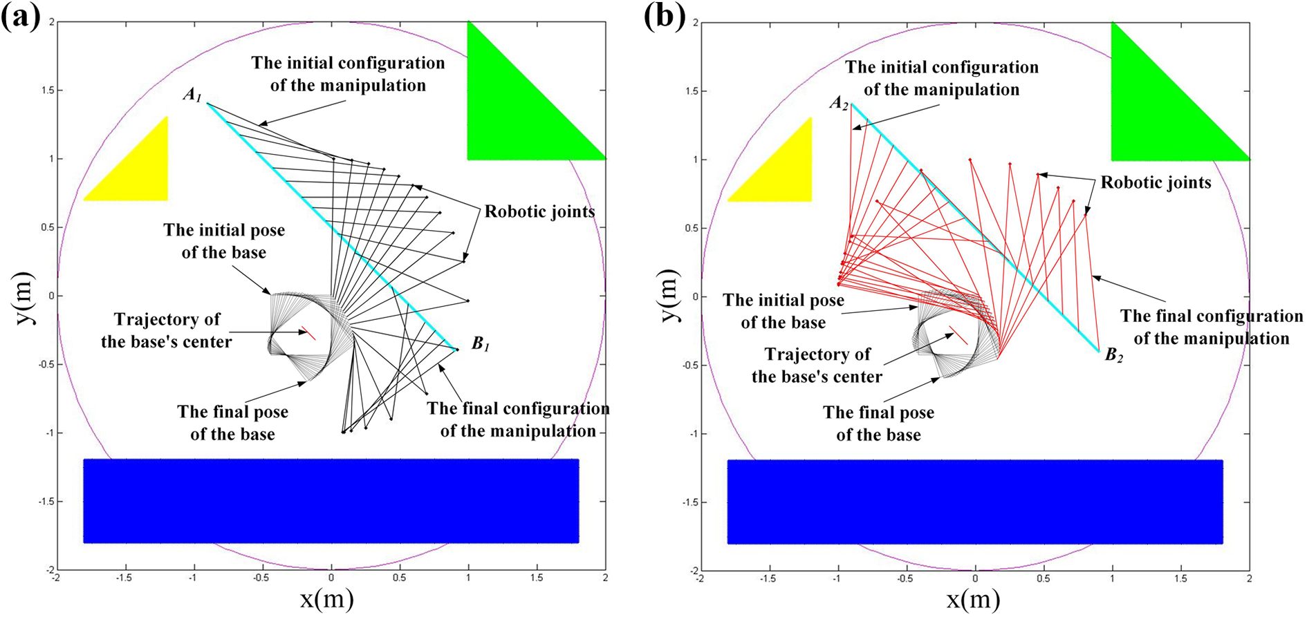
Based on the hybrid map in the Configuration space, optimization experiment of path planning is designed in this part. During the simulation experiment, the path planning moves from the start point A to the end point B in Figure 12. Due to the multi-solution property of the inverse kinematics, the start point A in Cartesian space corresponds to A ₁ and A ₂ in the Configuration space, while the end point B corresponds to B ₁ and B ₂. The obstacle avoidance and shortest path are used as constraints, and the artificial potential field method is used as the path planning algorithm. After the heuristic search strategy, two trajectories in red and black are searched out as shown in Figure 15. Both trajectories have achieved obstacles avoidance. However, the black path traverses ‘Hot Zone’ in the coupling map, disturbing the base more than the red path.

Figure 15.

Simulation results of path planning.

Figure 16 shows the configuration changes of the space robot in the Cartesian space. Figure 16(a) shows the configuration change of the robot corresponding to the black path A ₁ B ₁ in Cartesian space, while Figure 16(b) is corresponding to the red path A ₂ B ₂. It can be obtained from the figure that both paths implement the obstacle avoidance and are the shortest path in the straight line. Through the variation of the base centroid and the configuration of the robot manipulator, we can also intuitively feel that the disturbance in Figure 16(b) is more severe than in Figure 16(b).

Figure 16.

Configuration changes of the space robot. (a) The black path and (b) the red path.

The curves of the joint angles of the black path and the red path are depicted in Figure 17. We can conclude that the curves of the joint angles are smooth without singularity, which is in line with our previous analysis.

Figure 17.

The curves of joint angles.

In the above discussion, we measure the pros and cons of the two trajectories qualitatively. In order to quantitatively evaluate the path, based on the numerical hybrid map, this section designs the following evaluation criteria

E v a = \sum_{θ_{1}, θ_{2} \dots θ_{n}} h (θ_{1}, θ_{2} \dots θ_{n})

When the path planning is completed, the Eva obtained by different paths can be sorted, and the smallest Eva is selected as the optimal path. After calculation, the Eva of the black path is 0.9015 and the Eva of the red path is 0.7132. Therefore, the red path is chosen as the optimal path according to our rules.

Constraint for path planning

The core idea of the article is to build a map for path planning, and the path planning algorithm has not been considered. Therefore, the article uses the artificial potential field method mentioned by Liu et al.²⁰ as the path planning algorithm, and designs the potential functions of obstacles and coupling factors respectively. In this section, we present detailed comparisons of the hybrid map method with the method proposed by Liu et al.²⁰ In the following section, the method by Liu et al.²⁰ is referred to as the Liu method for the convenience of description.

Based on the map of Figure 14, the robot searches the path from the start point S to the end point G using our method and the Liu method, respectively. In the process of searching for the path, the robot is affected by three potential fields including obstacles, coupling factor, and the goal. Figure 18 shows the path planned by the Liu method and our method.

Figure 18.

Simulation results of path planning.

As shown in Figure 18, both paths can avoid obstacles. In terms of disturbances, the path planned by the Liu method passes through more “Hot Zone” than our method, indicating that the disturbance between the manipulator and the base is much severely. However, from the perspective of the path length, the planning path of the Liu method is slightly shorter.

In the following section, this article quantitatively measures the above methods. The three indicators, including obstacle avoidance, coupling disturbance and path length, are selected as the evaluation criteria of the path. The verification results are shown in Table 3.

Table 3.

Comparison of planning path indicators.

Indicator	Obstacle avoidance	Coupling factor	Eva	Path length (m)	Comprehensive performance
The Liu method	Yes	0.8536	0.7625	3.4245	0.8537
Our method	Yes	0.6779	0.5843	3.5372	0.7148

Eva: evaluation criteria.

The two paths are converted back to the Cartesian space and the length of the path is calculated. The length of path planned by the Liu method is 3.4245 m, while the length of path planned by our method is 3.5372 m. Taking the equation (43) as the criterion for evaluation, the Eva values of the two curves are calculated separately. The Eva of the Liu method is 0.7625, while the Eva of our method is 0.5843. Finally, the path length and Eva are normalized and weighted average to obtain comprehensive performance. The comprehensive performance of the Liu method is 0.8537 and our method is 0.7148. Therefore, considering the obstacle avoidance, coupling disturbance and path length, the article considers our method to be superior to the Liu method.

Although the experiment is based on a two degree-of-freedom planar space robot, the method can be applied to other multi-joint robot in the real world. The basic idea of the method is to build maps for path planning in the Configuration space, which can avoid the infinite solution of inverse kinematics. Once the path planning in the Configuration space is over, we will convert the path from the Configuration space to the Cartesian space to guide the control of the robot.

Conclusion

In order to build maps for path planning of free-floating space robot, a unified method dealing with the coupling minimization as well as obstacles avoidance is proposed in this article. The basic idea here is to optimize a path in the Configuration space by utilizing a hybrid map which consists of a coupling map and an obstruction map. The former generates from the value of the coupling factor derived from the spectral radius of the coupled matrix versus generalized coordinates; while the latter is developed from a conversion between two manifolds: the Cartesian space and the Configuration space. Thus, by overlaying these two maps, a novel hybrid map on which the search for an optimal path is conducted can be obtained. A two degree-of-freedom planar space robot is considered as a numeric demo in the simulation to evaluate the performance of our method. According to the results, our method is superior to the Liu method in terms of comprehensive performance. The proposed method provides maps for path planning and can be applied to space robots with any joint due to its robustness and universality. However, since our approach simplifies the model of obstacles, its performance deteriorates in applications of dynamic scenes

Footnotes

Declaration of conflicting interests

The author(s) declared no potential conflicts of interest with respect to the research, authorship, and/or publication of this article.

Funding

The author(s) disclosed receipt of following financial support for the research, authorship, and/or publication of this article: This work is funded by the National Natural Science Foundation of China (no. 11402004).

ORCID iD

Xiaodong Hu

References

Flores-Abad

Pham

. A review of space robotics technologies for on-orbit servicing. Prog Aerosp Sci 2014; 68: 1–26.

Chen

Meirovitch

. Control of a flexible space robot executing a docking maneuver. J Guid Control Dynam 1995; 18(4): 756–766.

Liu

Liang

Wang

. Autonomous path planning and experiment study of free-floating space robot for spinning satellite capturing. In: 13th international conference on control automation robotics & vision (ICARCV), Piscataway, USA, 2015, pp. 1573–1580. IEEE.

Green

Sasiadek

. Intelligent tracking control of a free-flying flexible space robot manipulator. In: Navigation and control conference, AIAA Guidance, Hilton Head, South Carolina, 2007, p. 6320.

Yoshida

. Experimental study on the dynamics and control of a space robot with experimental free-floating robot satellite. Adv Robotic 1994; 9(6): 583–602.

Moosavian

SAA

Papadopoulos

. On the kinematics of multiple manipulator space free-flyers and their computation. J Field Robot 1998; 15(4): 207–216.

Huang

Zhang

. Dynamics and configuration control of the maneuvering-net space robot system. Adv Space Res 2015; 55(4): 1004–1014.

Zhao

Bai

. Dynamics analysis of space robot manipulator with joint clearance. Acta Astronaut 2011; 68(7): 1147–1155.

Liu

Liang

. Autonomous path planning and experiment study of free-floating space robot for target capturing. J Intell Robot Syst 2008; 51(3): 303–331.

10.

Kumar

Pathak

Sukavanam

. Trajectory control of a two DOF rigid–flexible space robot by a virtual space vehicle. Robot Auton Syst 2013; 61(5): 473–482.

11.

Wang

Luo

Walter

. Trajectory planning of free-floating space robot using Particle Swarm Optimization (PSO). Acta Astronaut 2015; 112: 77–88.

12.

Zhang

Zhou

. Nonholonomic motion planning for minimizing base disturbances of space manipulators based on multi-swarm PSO. Robotica 2017; 35(4): 861–875.

13.

Vafa

Dubowsky

. The kinematics and dynamics of space manipulators: the virtual manipulator approach. Int J Robot Res 1990; 9(4): 3–21.

14.

Umetani

Yoshida

. Resolved motion rate control of space manipulators with generalized Jacobian matrix. IEEE T Robotic Autom 1989; 5(3): 303–314.

15.

. The measure of dynamic coupling of space robot systems. In: Proceedings of the IEEE international conference on robotics and automation, Atlanta, GA, 1993, pp. 615–620. IEEE.

16.

Shum

. Dynamic control and coupling of a free-flying space robot system. J Field Robot 1994; 11(7): 573–589.

17.

Peng

Liang

. Hybrid modeling and analysis method for dynamic coupling of space robots. IEEE Trans Aero Elec Sys 2016; 52(1): 85–98.

18.

Lozano-Perez

. Spatial planning: a configuration space approach. IEEE Trans Comput 1983; 2: 108–120.

19.

Wang

Luo

Walter

. A non-linear model predictive controller with obstacle avoidance for a space robot. Adv Space Res 2016; 57(8): 1737–1746.

20.

Liu

Zhang

Zhou

. Obstacle avoidance path planning of space manipulator based on improved artificial potential field method. J Instit Eng 2014; 95(1): 31–39.

21.

Luo

Zong

Wang

. Optimal capture occasion determination and trajectory generation for space robots grasping tumbling objects. Acta Astron 2017; 136: 380–386.

22.

Zhang

. Robust adaptive control of a free-floating space robot system in Cartesian space. Int J Adv Robot Syst 2015; 12(11): 157.

23.

Guo

Chen

. Adaptive robust control for free-floating space robot system with dual-arms to track desired trajectory in joint space. J Syst Simulat 2009; 3: 002.

24.

Jia

Misra

. Robust trajectory tracking control of a dual-arm space robot actuated by control moment gyroscopes. Acta Astron 2017; 137: 287–301.

25.

Wang

. Study on non-holonomic Cartesian path planning of a free-floating space robotic system. Adv Robot 2009; 23(1–2): 113–143.

26.

Zhao

Lü

. Smoothing obstacle avoidance path planning based on C-space for harvesting robot. In: Proceedings of the 32nd Chinese control conference, Xi’an, P. R. China, 26–28 July 2013.

27.

Raheem

Hussain

. Modified C-space analysis and construction for two-link robot arm. In: 1st International conference for engineering research, Middle Technical University, Baghdad, Iraq, March 2017.

Coupling minimization with obstacles avoidance of free-floating space robots based on hybrid map in configuration space

Abstract

Keywords

Introduction

Kinematic modeling and coupling effect analysis

Kinematic modeling

Coupling factor

Hybrid map in the configuration space

Coupling map in the configuration space

Obstruction map in the configuration space

Hybrid map in the Configuration space

Simulation experiment

Generation of the hybrid map

Generation of the coupling map

Generation of the obstruction map

Generation of the hybrid map

Experiment of path planning

Evaluation criteria of path planning

Constraint for path planning

Conclusion

Footnotes

Declaration of conflicting interests

Funding

ORCID iD

References