
Abstract
This article puts forth a framework using model-based techniques for path planning and guidance for an autonomous mobile robot in a constrained environment. The path plan is synthesized using a numerical navigation function algorithm that will form its potential contour levels based on the “minimum control effort.” Then, an improved nonlinear model predictive control approach is employed to generate high-level guidance commands for the mobile robot to track a trajectory fitted along the planned path leading to the goal. A backstepping-like nonlinear guidance law is also implemented for comparison with the NMPC formulation. Finally, the performance of the resulting framework using both nonlinear guidance techniques is verified in simulation where the environment is constrained by the presence of static obstacles.
Keywords
Introduction
The focus of this article is to present a framework for path planning and guidance for autonomous mobile robots. The framework is designed as a step toward increased autonomy for differential drive mobile robots. The quantifiable measures of autonomy the authors recognize in this article are the vehicle’s ability to observe, orient, make decisions, and act. 1 Of those autonomy measures, this article will focus primarily on expanding a mobile robot’s ability to make decisions and to control its actions within a given environment.
The first component of the framework discussed in this article is the navigation function (NF) path planner. NF planners are designed as a special class of artificial potential functions (APFs), wherein the local minimum problem is eliminated. In fact, within the potential field of a NF, there exists a unique global minimum located at an objective destination in the given environment. 2 –4 And there are two main approaches found in the literature for constructing a suitable NF.
The first method is to define an analytic function which possesses an attractive component associated with the objective and repulsive components attached to the obstacles. These approaches are motivated by the research introduced by Khatib 5 for online collision avoidance using APFs. Examples of the analytical approach with an NF are presented in previous studies, 6 –8 whose results originate from the NF definition introduced by Rimon and Koditschek. 4 With this approach, the NF is defined as a composition of several functions each designed to satisfy specific properties established by Rimon and Koditschek. 4 And while effective, this method requires proper tuning of several parameters within the function before the local minima can be removed and for the NF to be properly defined.
The second approach is to define the NF numerically in a discrete environment. Examples of this approach come in two flavors, either through wavefront expansion as described in previous works 2,3,9,10 or through numerical solutions to harmonic partial differential equations (PDE) as put forth in the literature. 11 –13 With the harmonic PDE methods, the boundary conditions of the numerical solvers are set for the obstacles and the objective to form a potential field with its unique and global minimum at the goal. In contrast, the wavefront expansion method identifies the goal and expands its potential through the free space and is computed based on the distance from the goal. 2,3 Also, with the numerical approaches, the path plans are typically determined through a graph search method such as the best first graph search method.
The path plan algorithm presented in this article expands upon earlier results by the authors. 14 Our approach is based on the the wavefront expansion algorithm. However, in the original wavefront expansion, as described by Latombe, 2 a distance-based metric from the goal is used to form the potential levels of the NF. With the new method, the potential contours are formed with a minimum control effort metric. Ultimately, this approach is dependent upon the kinematic model of the system being studied (model-based wavefront expansion method).
Other path planning techniques that make use of the control effort and the kinematic model of the system are discussed in terms of rapid exploring randomized trees (rrt and rrt*), 15,16 kinodynamic rrt, 17 and probabilistic roadmap approach. 18 These methods use a randomized approach with state information of the system to determine the path plans, and the paths are designed with information of the environment and the initial location. While these methods can be computationally intensive, depending on the model, they also generate plans without needing to know where the objective is located.
In contrast, the path plan algorithm introduced in this article can generate reference paths from anywhere in the free environment. However, the algorithm will require knowledge of both the objective location as well as a final desired state and would need to be regenerated if a new objective is given. The result, however, is a path plan that will guide the robot safely to its objective, while also considering the control effort to get there as well as how to form its approach to a goal state. Additionally, the path plan algorithm enables the inclusion of the kinematics of the mobile robot in its formation without increasing the dimensions of the configuration space of the system. The planner in this article considers the model of the mobile robot to consist of four state variables, but it generates the path plan within a two-dimensional environment making it computationally cheap.
The second component of the framework put forth in this article is the generation of high-level guidance commands based on a nonlinear model predictive control (NMPC) design. This approach is used to generate high-level guidance commands for the mobile robot to track a given trajectory. The derived guidance commands will be unique since it will make use of the state-dependent coefficient (SDC) form of the nonlinear kinematic equations, and the system’s inputs will be found by quadratic programming. The SDC formulation is used because it can preserve the nonlinear nature of the system being studied.
The use of model predictive control, or receding horizon control (RHC), is a widely researched topic in controls engineering for a variety of applications. Model predictive control is a process control method where the current inputs to the system are determined by forecasting the behavior of the system model over a finite horizon. The control is designed to minimize a cost function over the finite horizon and can be used for regulation or tracking of a reference trajectory. 19 Traditionally, NMPC involves linearizing the system’s dynamics about a nominal trajectory. 19 –21 Kwon and Han 19 and Rawlings 20 give an overview of the traditional formulation for NMPC.
The SDC form for nonlinear systems as it pertains to controller, observer, or filter design is discussed previous research. 22 –25 The focus of using the SDC form is to transform a nonlinear system into a psuedo-linear form and then implement optimal control or estimation techniques through solving the state dependent Riccati equation (SDRE). As it relates to control design, the SDC form allows for the synthesis of nonlinear feedback controllers that are similar to the linear quadratic regulator (LQR) structure.
The SDC form and control designs using the SDRE discussed by researchers 22 –25 center on solutions over an infinite time horizon for LQR types of problems. In contrast, the results described by Heydari and Balakrishnan 26 and Khamis and Naidu 27 look at solutions for control problems with a finite horizon. Both papers include a change of variables to solve for the control over a finite horizon as well as fixed terminal constraints, so that they can achieve their respective objectives. 26,27
In general, studies 22 –27 highlight the use of the SDC form and the nonlinear feedback control laws that can be found through solving the SDRE. These results, however, do not consider constraints on the system’s inputs or outputs (other than some terminal constraints, shown in previous studies 26,27 ). The novelty of the contribution of this article, using the SDC formulation and NMPC, is that it will enforce both input and output constraints while performing reference trajectory tracking.
An alternate approach for NMPC using an SDC approach employs a Control Lyapunov Function (CLF) to help with achieving stability and applying an approximation of the terminal cost to the tail of the infinite horizon problem. 28 –33 The CLF approach for RHC along with an SDC-factorized system is shown by Sznaier and colleagues, 30,31 without considering constraints. Primbs 28 presents the CLF technique in detail with RHC and focuses on time varying and input constrained systems. Jadbabaie 29 also covers the CLF approach with RHC, where the developments pertain to the stabilization of an unconstrained nonlinear systems and use the CLF as a terminal cost function.
The contribution of this component of the framework covered in this article is motivated by the developments of Ru and Subbarao. 34 However, the research presented distinguishes itself in that the NMPC guidance design is applied to a wheeled mobile robot which is verified in simulations. Overall, the contribution from this aspect of the work comes from the application of a combined planning and guidance scheme to a mobile robot vehicle and its comparison with another nonlinear guidance design based on backstepping.
Problem description
The proposed framework in this article will consist of two main capabilities meant to enhance the autonomous capabilities of a mobile robot. Figure 1 illustrates the main flow of information in a typical guidance, navigation, and control framework. The main contributions in this article will be in the areas of a NF path planner and two different nonlinear guidance designs, as highlighted in Figure 1. For the results given, it is assumed that information concerning the environment such as obstacle positions and objectives are known to the vehicle and that the maneuvers occur within a flat environment.

Block diagram depicting general guidance, navigation and control (GNC) framework.
The first capability of the framework evident with the path planning algorithm is that it has the ability to guide the vehicle safely through a hazardous, obstacle laden environment to a reachable state. This aspect of the work will be addressed through a special class of APFs called NFs. The objective with this component of the framework is to introduce the technique with the vehicle’s kinematic model and to generate a path plan that directs the approach of the vehicle to a final desired reachable state.
The second capability is the guidance law which generates high-level commands to have the vehicle track a desired path through the environment. This aspect within the framework is handled through two different nonlinear guidance techniques. The first technique is based on a NMPC derivation and the second is a backstepping-based design. The NMPC technique applied in this framework is given in “SDC-based NMPC” section of this article and is based on the developments found by Ru and Subbarao. 34 For this methodology, the SDC form is used to preserve the nonlinear nature of the vehicle’s kinematic equations and the weight on the terminal state of the system is found by solving the discrete time SDRE. The guidance commands are then found by quadratic programming with input and state constraints enforced on the system.
Then, the backstepping guidance law in this framework is presented in the “Nonlinear guidance law” section of this article. This approach is chosen for comparison with the NMPC design as it is an extensively studied method used for controlling differential drive mobile robots. This guidance law is designed to provide stable, high-level guidance commands and will be verified through simulation.
The simulation results involve the combination of the NF path planner with the nonlinear guidance designs to close the loop of the framework. The overall contributions of this article are to first present the path planning algorithm considering the kinematic model of a two-wheeled mobile robot. Second, this article will provide insight into the capabilities of two different nonlinear guidance techniques while tracking a reference trajectory fitted along a path plan through an obstacle laden environment.
Kinematic model of the mobile robot vehicle
The kinematic model of the vehicle is illustrated in Figure 2. For the results discussed, an East-North-Up convention is used. The heading angle, ψ, is defined positively going in a counterclockwise direction about the z-axis (up) going from the inertial x-axis (xI) to the body x-axis (xb). The state of the vehicle is taken as the inertial x and y position, its heading angle (ψ), and its forward velocity (v), and it can be represented by the vector

Kinematics of the robot vehicle.
The set of nonlinear kinematic equations used to represent the mobile robot are given by

where u1 and u2 are the guidance commands. These equations can be used as a representative model with control over the heading angle turn rate and the vehicle’s forward acceleration. The set of equations defined in equation (1) are used for the path planning algorithm and the nonlinear guidance derivations.
The equations of motion given in equation (1) also need to be placed in linear state-space form for use in the path planning algorithm. The linear equations of motion are placed in the form

where the

and

For the path planning algorithm, the nominal trajectory for the robot is considered as a straight line, non-accelerating trajectory between two points in a grid over a constant sample time,


Within the path planning algorithm, the values for
Path plan algorithm
The main contribution of this research is the construction of the NF, which is motivated by the wavefront expansion described in previous studies. 2,3 However, the novel design discussed here distinguishes itself from the traditional methods, since it will use a metric based on the control effort of the system to form the contour levels in the potential field as opposed to a distance-based metric. The work presented in this article expands on the previous results 14 by studying the linear kinematic model of a mobile robot and observing how it influences the potential contour levels with the algorithm. The end result is a path plan algorithm that is model-dependent.
The full algorithm is outlined in Figure 3 with the contributions to the algorithm highlighted. These modifications were added to the original wavefront expansion algorithm to enable the inclusion of a metric defined by the control effort of the system and allow for some constraints to be considered.

Control effort-based NF algorithm. NF: navigation function.
The method introduced in this article will make use of the solution to the minimum control effort problem given a fixed initial and final state for a linear system. This method is constructed to plan a path to an objective reachable state, expressed as
Minimum control effort approach
The minimum control effort–based path plan is designed considering the solution to the optimal control problem for finding the minimum energy controller. The cost function associated with this problem is given by

subject to

Within the context of the grid-based path planner, the above expression represents the cost going from one grid point at t0 to a neighboring grid point at tf (denoted as

where

and the reachability Gramian is computed by
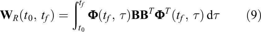
which needs to be non-singular in order for the state at tf to be reachable.
Solving for the reachability Gramian using equation (9) is not straightforward; however, there are simplifications to find a solution which exist in the linear systems literature, such as the study by Chen. 36 One method to find a solution to equation (9) is to look at the analytic solution of a differential Lyapunov equation. The solution to the differential Lyapunov equation of the form

is given by

Therefore, by taking
Additionally, the aspect of reachability for the system being studied is formally addressed with the following remark. The motivation for this assertion can be found in the discussions of chapter 6 in the study by Chen 36 and chapter 3 in the study by Williams and Lawrence 37 involving the concept of a system’s controllability and its implications with regards to reachability. The aim is to show that if the linear system is controllable, then it can be directed to successive local reachable states, with each one leading the system to the final objective reachable state at the end of the path plan.
Remark 1
Consider the nonlinear system in equation (1) and it’s linearization in equation (2) about the nominal state,
In equation (2), the input vector,


Grid set up in two-dimensional space for a mobile robot model.
And the nominal velocity is computed as

To compute the control effort from equation (8), the state information at t0 and at tf needs to be determined. Within the path planning algorithm, the final state at each level is taken as the ith state extracted from the kth list, that is,
At t0, the state information is denoted as
and the velocity as

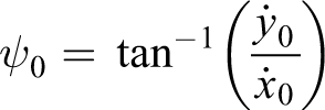
where the directional velocities are calculated as


where
Finally, in order to make use of the solution to the minimum energy controller in equation (8), the state perturbations
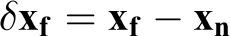

This procedure is done for each of the free neighbors of
Initialization block
Now, with an understanding of how the minimum energy controller influences the potential levels in the NF, an explanation of the modified wavefront expansion is given. The first step of the algorithm takes place with the initialization block, as shown in Figure 3.
The initialization block of this numerically constructed potential field begins by discretizing the workspace into an evenly spaced grid. This grid can be scaled to fit over any two-dimensional working environment. The discrete grid and the obstacle positions are then used to form a bitmap representation of the environment. This allows the free points to be identified and extracted. Note that the free space is denoted as
Also, during initialization, the obstacle potential levels are set uniformly to a large number and these configurations are separated for the rest of the algorithm. The potential level of the desired final state is then set to zero, to ensure that it is the global minimum, and these values are inserted into a list, list
k
, where the index k = 0 initially, that is,
Another attribute that is set during initialization is the model to base the NF generation. The model will motivate how to set the final objective state,
Main block
Once set, the information from the initialization block is passed into the algorithm’s main block to generate the NF. Within the algorithm, the states and potentials within list
k
are used to evaluate the potential values of their neighbors,
Next, it must be determined if the neighbor point is in the free space and if the potential has not yet been computed. If the neighbor point is both free and has not been visited by the wavefront expansion, then the algorithm continues; otherwise, that point is disregarded and the next neighbor point,
Also, for the free neighbor points, the algorithm completes the state information of
The resulting control vector and position information are compared with the constraints


where
Effectively, the deff term in equation (13) does make this method partially dependent on a measure of distance. However, the deff term is associated solely with the maximum control effort constraint, umax. The combination of the constraints in equations (12) and (13) is used to enforce the notion that it would be cost prohibitive to approach the final desired state from certain configurations, such as facing the opposite direction at close proximity. The deff parameter in this sense restricts the umax constraint to only affect grid points within a certain neighborhood of the goal and has no bearing on the potential levels through the rest of the free space.
Now, if the constraints in equations (12) and (13) are violated at a given neighbor point,

where
There are a couple of considerations with the cost function in equation (14). The first is that the cost is always increasing from one level to the next with the wavefront expansion, and this feature is what enables us to claim that there is a unique and global minimum at the goal. Second, the choice of grid resolution, or the spacing between the grid points, and the time-step parameter
Finally, when the cost for

in Figure 3. This process is continued for each neighboring configuration of
If all the neighbors have been visited, then the next final state and cost in list
k
are used, that is,
Once the NF algorithm finishes, the reference path,
The resulting path plan is used to provide a set of reference position coordinates,
SDC-based NMPC
The primary guidance technique discussed in this article uses a NMPC approach and is presented in this section. The procedure is motivated by the work of Ru and Subbarao, 34 where the performance of the traditional approach of NMPC is compared with that of a SDC approach. The objective in this section is to present this method for an autonomous mobile robot and verify its trajectory tracking capability in simulation and then compare its performance with the results from a different and widely researched nonlinear guidance approach.
SDC representation of the vehicle kinematics
Given a general nonlinear system of the form

a state-space representation of the system is obtained wherein the system matrices are given as functions of the current state of the system as
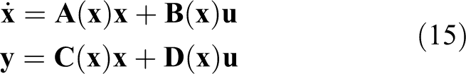
where
In general, the formation of SDC matrices for the system are not unique unless observing a scalar system. 22 –25 Therefore, different SDC forms may be obtained for a given system and solutions to the optimization problems posed may vary. Two particular SDC factorizations of the kinematics, from equation (1), are derived for the results in this article.
For the results, it is assumed that the full state is available at each instant, that is, the system output matrix

And one possible solution for the SDC factored

where

This result is derived using the following trigonometric identity and expansions
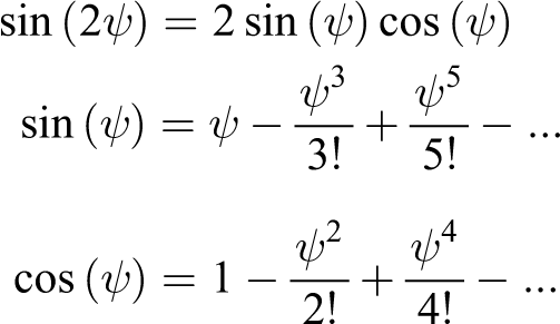
The above derivation of the

Note that with both SDC matrix results from equations (17) and (18), the psuedo-linear system
Next, a discrete-time equivalent of the system shown in equation (15) can be obtained by introducing a zero-order-hold (ZOH) with a specified sample time (

where
The discrete-time system in equation (19) can be placed in batch form for an N-step prediction horizon as

where


And the terminal state at the end of the prediction horizon is defined as

where

NMPC design
The guidance commands are obtained as the solution to the minimization of the finite-horizon linear quadratic tracking cost function with free final state subject to state and input constraints. The cost function is given as

where

where

is the batch form of the reference trajectory over the N-step horizon and
After proper substitution, the objective function can be rewritten in a quadratic-like form as

The objective function depends on the current state of the system and is calculated at the beginning of every sample interval. Also, the weight matrix for the final state,
where
Input and state constraints
The constraints are used in this formulation to ensure that the tracking capabilities of the system are feasible in simulation and in practice. The nonlinear kinematic equations for the vehicle represented in equation (1) enable constraints to be placed on the heading angle turn rate and acceleration of the vehicle without added complication. Overall, the form of the kinematics chosen enables us to place constraints on the system’s velocity, heading angle, its turn rate, and its forward acceleration. In general, the input and state constraints are represented by the following inequalities
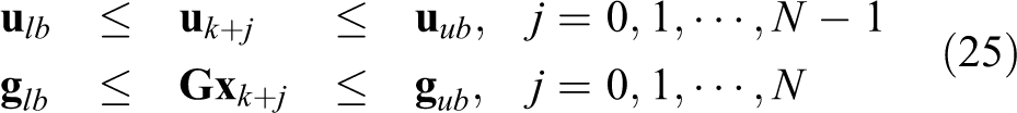
where the subscripts lb and ub denote the lower and upper bounds, respectively, of the constraints and the matrix

where

where

and

where

The guidance commands are synthesized by minimizing the quadratic cost function in equation (23), subject to the input and state constraints in equation (27) using quadratic programming.
Guidance command synthesis using the linear matrix inequality form
For readability with the following linear matrix inequality (LMI) formulation, the notation for state dependence is changed from using brackets to a subscript, in other words

where

and

Then, for each

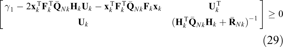


where

subject to the constraints in equations (29) to (32). And upon solving the quadratic programming problem,

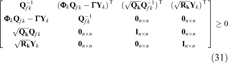
which will extract the guidance commands corresponding to the kth time step to the system in equation (1). The stability of the closed-loop system using the SDC-based NMPC guidance law is given in Appendix 1.
Nonlinear guidance law
The second guidance technique investigated with this research is a backstepping-based approach which is chosen for comparison with the NMPC design for generating guidance commands for the mobile robot. Unlike the guidance law design using NMPC, the derivation in this section will not explicitly introduce constraints into the formulation.
Using the kinematic equations for the vehicle defined in equation (1), the guidance commands u1 and u2 influence the turn rate and forward acceleration of the robot. The guidance commands defined using the backstepping-based approach are


where
The guidance commands are formulated to achieve stability in the sense of Lyapunov while tracking a reference trajectory. Note, the position tracking errors are given by
Then, using equation (36), the desired heading angle and velocity signals are obtained as


The guidance commands are derived such that the heading angle and velocity tracking errors,

which are the terms introduced in equations (34) and (35).
The time derivatives for the desired heading angle and velocity values are obtained by differentiating equations (37) and (38) with respect to time, leading to


where
Note that when vd = 0,


The values of

where n is the number of position points in the reference trajectory and the ordered pair
Simulation results
The examples presented in this article are based on a two-dimensional Euclidean workspace. It is assumed that knowledge of the workspace such as the obstacle regions, model properties, and the objective reachable state are known by the robot. It is important to note that the path plan in both scenarios would have to be regenerated if either the environment or objectives change, thereby making the algorithm inefficient. However, the focus of this article considers situations where there are little to no uncertainty in the environment, such as in a warehouse or an open space and the objective is well defined.
There will be two example environments shown. The first case will have no obstacles present which will illustrate the features of the potential field’s formation with the NF algorithm. Then, the second case will have obstacles present in the environment which will be used to demonstrate the obstacle avoidance capability of the algorithm. A trajectory is fitted over the path plans as described in Appendix 1 and is used to test the trajectory tracking performance of the two guidance designs for both cases.
In this section, the path plan algorithm results will be shown first. With these set of results, the path plan will be shown alongside a contour plot illustrating the potential levels the algorithm generates. Next, the simulation results of the different guidance laws are presented with the same two cases tested using each design. The simulation results are obtained using MATLAB 2017a and the quadratic programming problem is solved using MATLAB’s solver in the optimization toolbox.
Path plan results
The results of the path plan algorithm are given in this subsection. The resulting path plan and potential levels are highlighted in each of the plots. Case 1 is the example with no obstacles in the environment and case 2 depicts an example environment with obstacles present.
Case 1: No obstacles present
For the first example, the final desired reachable state is
The NF algorithm is run considering the minimum control effort approach with a linear rover model, and the resulting potential field and path plan is illustrated in Figure 5.

Minimum control energy path plan and potential field for case 1.
The value of

Minimum control energy path plan and potential field for case 2.
Case 2: Obstacles present
The following example demonstrates the obstacle avoidance capability of the path planner with multiple obstacles present. The final desired reachable state for this example is taken as
The results with the path planner show that the paths generated will avoid collisions and direct the vehicle to a state in between two obstacles.
From the results, it can be seen that the potential fields only possess one global minimum. This is a result that comes from the wavefront expansion construction method used. This also implies that a path plan can be formed to the final state from any free configuration in the given environment.
Note that if a minimum distance based path plan approach were considered, particularly in the second result in Figure 6, the path plan would look different. The resulting path plan would go straight toward the objective and hug the boundary of the obstacles until it is safely around. With the minimum control effort-based approach, the robot is trying to reduce the control energy, making it so there are less changes in direction and that they are not as sharp or sudden.
Trajectory tracking results
For all the trajectory tracking results presented, the same path plan results are used. And the reference trajectory is generated along the path plan as described in Appendix 1 with a desired time to reach the goal set at
For the NMPC guidance law, the sampling time used to discretize the SDC system is chosen as

The input constraints chosen for the simulation are chosen as

for the heading angle turn rate and forward acceleration, respectively. The state, or output, constraints are placed on the heading angle and velocity, respectively, as

These constraints are chosen based on experiments conducted with the experimental mobile robot platform in the Aerospace Systems Laboratory at the University of Texas at Arlington. However, the lower bounds of 0.001 m/s for the velocity are chosen due to the lack of controllability with the SDC form of the equations (from equation (15)) when the velocity is equal to zero.
Then, for the backstepping guidance law results, the control gains are chosen as constants where
Case 1: Framework simulation results
The simulation results for case 1 are presented in Figures 7 to 12. The results illustrate the reference path tracking performance in Figures 7 and 8. Then, the simulated heading angle and velocity signals are depicted in Figures 9 and 10, respectively. Last, the guidance command time histories are shown in Figures 11 and 12 for u1 and u2, respectively. For the simulation results presented, the subscript NL denotes the set of results from the backstepping-based nonlinear guidance law and the subscript NMPC denotes the set of results from the NMPC guidance law.

Reference path tracking for case 1.

x. and y position tracking for case 1.

Heading angle plot for case 1.
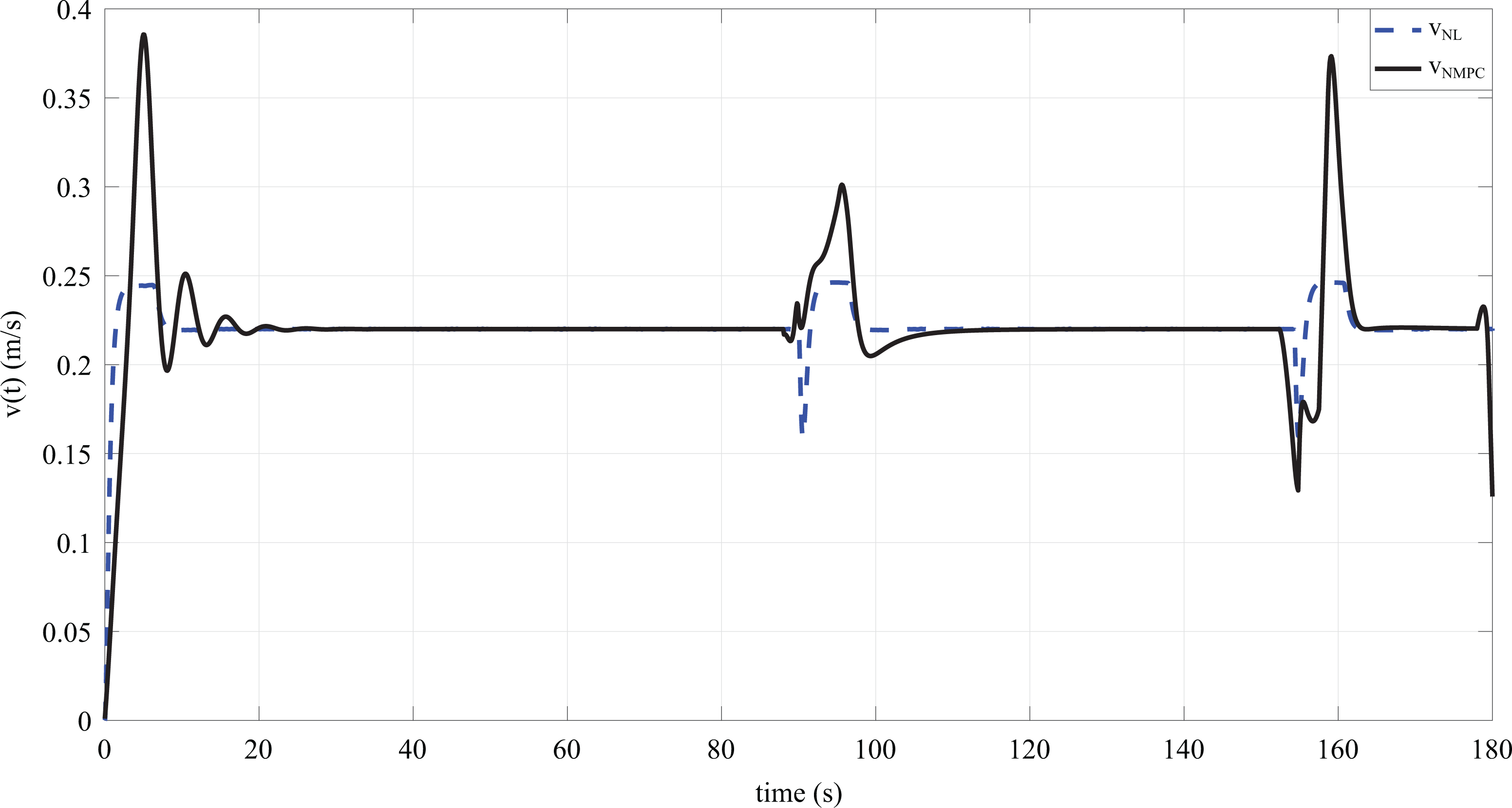
Velocity plot for case 1.

Guidance command u1 for case 1.

Guidance command u2 for case 1.
From the reference path tracking results in Figures 7 and 8, the performance of the two guidance laws are nearly identical. Both guidance laws tightly track the reference path given with each simulation result showing that the vehicle arrives at its objective location.
The different behavior of the two guidance designs is evident in the plots of the robot’s heading angle and velocity, Figures 9 and 10, respectively. In these plots, it can be seen that there are spikes in the signals which correlate to the corner points in the reference path where a sharp turn occurs. The NMPC signals spike higher than the backstepping signals at these times due to the constraints being considered. The constraints enforced (essentially the vehicle’s acceleration and the turn rate, see Figures 11 and 12) within the NMPC framework imply that it cannot settle to a steady value as suddenly as the backstepping designs, hence the overshoot in the signals. Additionally, there are oscillations in the velocity signal in Figure 10, these may be undesired and can be lessened with further tuning of the state and input weight matrices.
As highlighted previously, another important contrast between the two guidance laws is evident in the plots of the guidance command history in Figures 11 and 12. In these plots, the constraints enforced within the NMPC design are overlayed on the plot of the two signals. The results in Figures 11 and 12 illustrate that the guidance commands for the NMPC design obey the constraints of the system. In contrast, the backstepping guidance commands have sudden sharp changes over the course of the simulation which would violate these constraints.
Also, notice the behavior of the acceleration guidance command, u2, at the end of the simulation. At the end of the simulation, the guidance command drops suddenly to a low negative value. This occurs because the guidance law is commanding the vehicle to decelerate and stop at the end of the trajectory. The NMPC commands the vehicle’s acceleration to the lower bounds of its capability, whereas the backstepping command tends to a value that violates this constraint. This feature is also evident in the guidance command plot for case 2 in Figure 18.
Case 2: Framework simulation results
The simulation results for case 2 are presented in Figures 13 to 18. As with the previous case, the results illustrate the reference path tracking performance first in Figures 13 and 14. Then, the simulated heading angle and velocity signals are depicted in Figures 15 and 16, respectively. Last, the guidance command time histories for case 2 are shown in Figures 17 and 18 for u1 and u2, respectively.

Reference path tracking for case 2.

x. and y position tracking for case 2.

Heading angle plot for case 2.

Velocity plot for case 2.

Guidance command u1 for case 2.

Guidance command u2 for case 2.
Similar to the simulation results in case 1, the reference path tracking performance with both guidance laws are indistinguishable, as illustrated in Figures 13 and 14. The differences of the two methods are most evident in the simulation results of the heading angle, velocity, and guidance command signals, depicted in Figures 15 to 18, respectively.
As with the results for case 1, the heading angle and velocity signals of the two simulations behave similarly with the signals spiking at time instants that correlate to when the robot is making sudden turns along the reference path. The difference lies in the time it takes for the signals to settle. The backstepping signals settle rather quickly whereas the NMPC signals do so gradually. This behavior with the NMPC design is attributed to the constraints being enforced within its design. Similar to the result shown in Figure 10, there are oscillations in the velocity signal in Figure 16, and this behavior again may be lessened with further tuning of the state and input weight matrices.
Also, the guidance command history plots, shown in Figures 17 and 18, display similar results to what was presented with case 1. The guidance commands originating from the NMPC design are able to adhere to the constraints on the system over the duration of the simulation. In comparison, the backstepping commands again provide sharp and sudden changes which, at times, exceed the capabilities of the vehicle.
Overall, the guidance commands from the backstepping approach adhere to the constraints of the system for most of the simulation. However, the presence of sudden sharp changes in its guidance commands, as well as heading angle and velocity signals, could present complications in applying the backstepping approach to a mobile robot platform.
Conversely, all the state and input signals corresponding to the NMPC guidance law operate within the defined capabilities of the vehicle as intended. These signals do have some sudden changes but are less amplified in comparison with the backstepping approach over the course of the simulation. Thus, the capability of the NMPC design to ensure that the vehicle can operate within its physical limitations could prove beneficial for the kinds of tasks it may face.
Conclusions
In this article, a procedure for developing a reliable path planning and guidance framework for autonomous mobile robots was presented. The article introduced a new model-based path planning algorithm in addition to a NMPC guidance design to form a reliable path planning and guidance framework that was verified in simulation. The path planning algorithm, essentially derived from a special form of an APF constructed based on the minimum control effort to a goal state was shown to be very effective in synthesizing trajectories by transitioning through locally reachable states. The trajectory design exploited the wavefront expansion construction procedure to form potential contours using a control effort-based metric, thus establishing a model-based minimum control effort trajectory. This approach enables one to find an obstacle-free path that not only guides a robot to its objective state but also takes into account the final approach of the vehicle to a reachable state. Additionally, this algorithm allows for the obstacle-free paths to be formed from anywhere in the environment. The guidance law using the SDC-based NMPC design explicitly accounts for the vehicle’s physical constraints to track the desired trajectory. Comparisons with a nonlinear backstepping-based guidance law show similar tracking performance but the NMPC clearly distinguished itself by being able to perform with realistic constraints imposed on the system.
Ultimately, the combination of the aspects described in this article form a model-based framework that can be used for path planning and guidance involving autonomous mobile robots.
Future work using the research presented in this article includes applying the derived methods to real-time mobile robot platforms. Additionally, a detailed comparison of the path planning algorithm with other techniques will be conducted and considered with the minimum control effort approach.
Footnotes
Declaration of conflicting interests
The author(s) declared no potential conflicts of interest with respect to the research, authorship, and/or publication of this article.
Funding
The author(s) received following financial support for the research, authorship, and/or publication of this article: The authors acknowledge support for this project provided by the Air Force Research Lab (AFRL) through award FA9453-16-1-0058.