An improved artificial potential field method of trajectory planning and obstacle avoidance for redundant manipulators

Abstract

In this article, we present an improved artificial potential field method of trajectory planning and obstacle avoidance for redundant manipulators. Specifically, we not only focused on the position for the manipulator end-effectors but also considered their posture in the course of trajectory planning and obstacle avoidance. We introduced boundaries for Cartesian space components to optimize the attractive field function. Moreover, the manipulator achieved a reasonable speed to move to the target pose, regardless of the difference between the initial pose and target pose. We proved the stability using Lyapunov stability theory by introducing velocity feedforward, when the manipulator moved along a continuous trajectory. Considering the shape of the manipulator joints and obstacles, we set up the collision detection model by projecting the obstacles to link coordinates. In this case, establishing the repulsive field between the nearest points on every joint and obstacles with the closest distance was sufficient for achieving obstacle avoidance for redundant manipulators. The simulation results based on a nine-degree-of-freedom hyper-redundant manipulator, which was designed and made in our laboratory, fully substantiated the efficacy and superiority of the proposed method.

Introduction

Redundant manipulators are mostly intended for performing complex tasks in a restrictive environment, because they have a high number of degrees of freedom (DOFs), and the flexibility that results from a high number of DOF. In particular, their end-effectors are required to follow a desired trajectory; meanwhile, none of their joints will collide with obstacles in any cases. Many ^{1 –20} approaches have been proposed to solve the problems of trajectory planning and obstacle avoidance.

Considering redundant manipulators that work in Cartesian space, they have more than six DOFs. Hence, every desired task pose (position and posture) corresponds to infinite joint configurations. Moreover, when redundant manipulators perform the main task of tracking a desired trajectory, they are required to avoid joint limits and singularities, evade obstacles, and minimize the tracking error as far as possible. To solve these issues, global and local strategies have been developed by some researchers. Global path planning is a relatively well-studied research area ¹ ; many global approaches were presented to solve these kinematic problems for redundant manipulators such as rapidly exploring random trees, ^2,3 graph search algorithms, ⁴ optimization of predefined paths, ⁵ tangent graph-based planning, ⁶ mathematical programming and optimization, ⁷ and partially observable Markov decision processes. ⁸ A free path and the joint variables are obtained through the application of restrictions such as obstacles and joint limits. However, since complete trajectory information needs to be offered in advance, global methods are not suited to tasks that require continuous trajectory modification based on sensory feedback. ⁹ Local strategies are utilized by applying the deformation of the Jacobian matrix to acquire the trajectory online step by step based on current information. Conventionally, to minimize the joint velocity norm under the premise of the minimum tracking error of the end-effector, the Jacobian pseudoinverse is defined as the general solution of redundancy resolution. ¹⁰ The gradient projection method based on the Jacobian pseudoinverse is used to obtain the self-motion necessary to optimize the performance criteria, such as the avoidance of the joint limit and obstacle by defining a standard function and projecting it onto the null space of the Jacobian. ^11,12 The weighted least-norm solution was suggested to minimize energy using the inertia matrix as the weighting matrix. ¹³ Additionally, it also can be used to avoid joint limits ¹⁴ and reduce joint torque. ^15,16 Another option was developed as a so-called augmented Jacobian approach ^17,18 and extended the Jacobian as a square matrix with additional tasks, such as performing cyclic tasks ¹⁹ and avoiding obstacles. ²⁰ The artificial potential field method concerned in this article is a kind of local strategy that exerts virtual forces that are caused by attractive potentials or repulsive potentials on the manipulator link or end-effector. ²¹ Hence, the global dynamics model of the manipulator is required and the friction forces also cannot be neglected. Another kind of potential field method is to calculate the joint velocities by introducing the Jacobian pseudoinverse ²² and avoid collisions by controlling the joint velocities in the Jacobian nullspace. ²³ The pseudo-distance between obstacles and links is defined to extend the Jacobian matrix to avoid collisions. ²⁴ However, in these artificial potential field methods, stability is always demonstrated only in point-to-point motion but seldom considered while end-effector moving along a continuous trajectory. Furthermore, if the difference between the initial pose and target pose is too large, then the motion mode may be impossible because of demanding high speed or large torque. When repulsive potentials are used for obstacle avoidance, the volume of the link is often neglected, but the shape of the obstacle or its effect on manipulator motion is always expanded. The approximate method of obstacles reduces the motion space of manipulators in their restrictive work space, and neglecting the volume of the link may also increase the risk of failure to avoid obstacles. Additionally, most of these potential field methods are verified using planar robots, ^{22 –24} the verification and application of the method is seldom considered in Cartesian space, and the continuous change of posture is also neglected.

In this article, we propose an improved artificial potential field method to achieve trajectory planning and obstacle avoidance. Both position and posture are controlled simultaneously by defining an optimized six-dimensional attractive field in Cartesian space. Moreover, the product of the Jacobian pseudoinverse and desired speed is used as feedforward while manipulators move along a continuous trajectory. Obstacle avoidance is transformed by the collision detection problem, and only the repulsive potential field between the nearest two points on the obstacle and joint is considered. The attractive force caused by the attractive field and the repulsive force caused by the repulsive field are converted to joint torques using the Jacobian transpose. The torques are translated into joint velocities by constructing the virtual relationship between them to achieve trajectory and obstacle avoidance.

The remainder of this article is organized as follows. In “Trajectory planning based on attractive potential” section, we describe the trajectory planning method for a redundant manipulator, which can offer a reasonable motion form for the end-effector from the initial pose to the target pose. In “Obstacle avoidance based on repulsive potential” section, we present the obstacle avoidance algorithm that introduces the simplified geometric model of the manipulator link and only considers the repulsive potential action between the closest points on the obstacle and link. We discuss the simulation results and analysis of the proposed trajectory planning and obstacle avoidance algorithm for the redundant manipulator in “Simulation results” section. Finally, we present the conclusions.

Trajectory planning based on attractive potential

In actual applications, the desired trajectory is given in Cartesian space, whereas the manipulator can only be controlled in the joint space. Hence, the main issue in this field is to define the relation between Cartesian space and joint space. In this case, an approach based on the forward kinematic and the Jacobian transpose is employed.

The principle of trajectory planning based on attractive potential is shown in Figure 1. The schematic diagram of the n DOF robot is drawn during its initial pose and dotted line in the target pose; however, the configuration of the joint that corresponds to the target pose is not unique. From the graph, the relation between the two poses is obtained as

$x_{\text{tar}}=x_{\text{ini}}+\Delta x$

1

where x_tar, x_ini, and Δx are the target pose, initial pose, and difference between the two poses, respectively, and they are all 6 × 1 vectors consisting of three translational and three rotational components. Thus, any pose of the end-effector can be written as

$x={\left[\begin{array}{cc}{x}_{\text{t}}& x_{\text{r}}\end{array}\right]}^{\text{T}}={\left[\begin{array}{llllll}x\hfill & y\hfill & z\hfill & \alpha \hfill & \beta \hfill & \gamma \hfill \end{array}\right]}^{\text{T}}$

2

where $x_{\text{t}}=[\begin{array}{lll}x\hfill & y\hfill & z\hfill \end{array}]$ and $x_{\text{r}}=[\begin{array}{lll}\alpha \hfill & \beta \hfill & \gamma \hfill \end{array}]$ , respectively, denote the translational pose and rotational pose. Moreover, we assume that there is a force F_att caused by the attractive potentials to pull (and twist) the manipulator end-effector toward the target pose. And the force F_att can enable a change in the orientation in addition to the position of the end-effector; hence, it is also a 6 × 1 vector.

Figure 1.

Schematic of redundant manipulator end-effector movement under the influence of attractive potential field.

As mentioned above, force F_att is caused by the attractive potential around the target pose. We describe how the attractive potential can be constructed directly on the end-effector of the manipulator. Attractive potential field U_att is constructed to make the end-effector be attracted to the target pose; hence there are some criteria that should be satisfied by field U_att. Clearly, U_att should be increasing with the difference Δx. However, if only the linear relationship between U_att and Δx is defined, then this will lead to stability problems, because there is a discontinuity near the origin at which attractive force F_att caused by potential field U_att tends to zero ^.25 To obtain a continuously differentiable potential field, such a field that grows quadratically with Δx is defined as

$\begin{array}{l}{U}_{\text{att}}={\left[\begin{array}{cc}{U}_{\text{t}}& U_{\text{r}}\end{array}\right]}^{\text{T}}\\ =\frac{\xi }{2}\left[\begin{array}{llllll}\Delta x^2\hfill & \Delta y^2\hfill & \Delta z^2\hfill & \Delta {\alpha }^2\hfill & \Delta {\beta }^2\hfill & \Delta {\gamma }^2\hfill \end{array}\right]\end{array}$

3

where $U_{\text{t}}=\frac{\xi }{2}\left[\begin{array}{ccc}\Delta x^2& \Delta y^2& \Delta z^2\end{array}\right]$ and $U_{\text{r}}=\frac{\xi }{2}\left[\begin{array}{ccc}\Delta {\alpha }^2& \Delta {\beta }^2& \Delta {\gamma }^2\end{array}\right]$ , respectively, denote the attractive potential which make the end-effector translate and rotate, and ξ is a parameter used to scale the effect of the attractive potential. The influence of every pose difference in Cartesian space is different, hence; ξ is a diagonal matrix rather than a constant; ξ is denoted as $\xi =\text{diag}\left({\xi }_1,{\xi }_2,{\xi }_3,{\xi }_4,{\xi }_5,{\xi }_6\right)$ . Moreover, F_att can be given as

$\begin{array}{l}{F}_{\text{att}}={\left[\begin{array}{cc}{F}_t& F_r\end{array}\right]}^{\text{T}}\\ ={\left[\begin{array}{llllll}{F}_x\hfill & F_y\hfill & F_z\hfill & F_{\alpha }\hfill & F_{\beta }\hfill & F_{\gamma }\hfill \end{array}\right]}^{\text{T}}\\ =\xi {\left[\begin{array}{llllll}\Delta x\hfill & \Delta y\hfill & \Delta z\hfill & \Delta \alpha \hfill & \Delta \beta \hfill & \Delta \gamma \hfill \end{array}\right]}^{\text{T}}\end{array}$

4

where $F_{\text{t}}=\left[\begin{array}{ccc}{F}_x& F_y& F_z\end{array}\right]$ and $F_{\text{r}}=\left[\begin{array}{ccc}{F}_{\alpha }& F_{\beta }& F_{\gamma }\end{array}\right]$ , respectively, denote the force which make the end-effector translate and rotate. Note that ${F_{\text{att}}}^i\left(i=1,2,\cdots \mathrm{,6}\right)$ converges linearly to zero with $\Delta x^i$ decreasing and grows without bound with $\Delta x^i$ increasing. Hence, if ${x_{\text{ini}}}^i$ is very far from ${x_{\text{tar}}}^i$ , then it may produce too large an attractive force ${F_{\text{att}}}^i$ . Thus, the quadratic and conic potentials are combined to define the attractive potential, and boundary η should be explained. When $\Delta x^i$ is over η, the conic potential works on the manipulator; otherwise, the quadratic potential attracts the manipulator. Clearly, the boundary of translational and rotational components cannot be defined by the same standard, so η is expressed as

$\eta ={\left[\begin{array}{cc}{\eta }_{\text{t}}& {\eta }_{\text{r}}\end{array}\right]}^{\text{T}}$

5

where η_t and η_r describe the boundary of translational and rotational components, respectively. Furthermore, U_att can be defined as

$\begin{array}{l}{U}_{\text{t}}^i=\{\begin{array}{cc}\frac{1}{2}\xi ||\Delta x^i|{|}^2& ||\Delta x^i||\le {\eta }_{\text{t}}\\ {\eta }_{\text{t}}\xi ||\Delta x^i||-\frac{1}{2}\xi {\eta }_{\text{t}}& ||\Delta x^i||>{\eta }_{\text{t}}\end{array}\\ \text{and}\hspace{0.17em}{U}_{\text{r}}^i=\{\begin{array}{cc}\frac{1}{2}\xi ||\Delta x^i|{|}^2& ||\Delta x^i||\le {\eta }_{\text{r}}\\ {\eta }_{\text{t}}\xi ||\Delta x^i||-\frac{1}{2}\xi {\eta }_{\text{t}}& ||\Delta x^i||>{\eta }_{\text{r}}\end{array}\end{array}$

6

and in this case F_att is given as

$\begin{array}{l}{F}_{\text{t}}^i=\{\begin{array}{cc}\xi \Delta x^i& \Vert \Delta x^i\Vert \le {\eta }_{\text{t}}\\ \xi {\eta }_{\text{t}}\frac{\Delta x^i}{\Vert \Delta x^i\Vert }& \Vert \Delta x^i\Vert >{\eta }_{\text{t}}\end{array}\\ \text{and} F_{\text{r}}^i=\{\begin{array}{cc}\xi \Delta x^i& \Vert \Delta x^i\Vert \le {\eta }_{\text{r}}\\ \xi {\eta }_{\text{r}}\frac{\Delta x^i}{\Vert \Delta x^i\Vert }& \Vert \Delta x^i\Vert >{\eta }_{\text{r}}\end{array}\end{array}$

7

The boundary is well defined for the two fields because both U_att and F_att are continuous in the entire field.

Specific attractive force F_att can be obtained from the attractive potential as defined above. Additionally, F_att acting on the end-effector is resolved to joint torque

${\tau }_{\text{att}}=J^{\text{T}}{F}_{\text{att}}$

8

where J is a 6 × n matrix, and n denotes the DOF of the manipulator, as a result, τ is an n × 1 vector. We assume that there are no joint motors only viscous dampers on the manipulator, thus, joint velocity $\dot{\theta }$ is proportional to the applied torques

${\dot{\theta }}_{\text{att}}=\frac{{\tau }_{\text{att}}}{B}$

9

where B is the joint damping coefficient (all dampers are assumed to be the same). ²⁶ The change in the joint angle is obtained through the joint speed integral, and based on this, we determine the trajectory to the target pose. The principle is as shown in Figure 2.

Figure 2.

Block diagram of point-to-point trajectory planning for redundant manipulator.

Gain K is denoted as $K=\xi /B$ . And the influence of pose difference Δx and the joint speed ${\dot{\theta }}_{\text{att}}$ can be controlled by adjusting the magnitude of K. Current pose x of the end-effector can be solved using forward kinematics according to the current joint angles. The stability of the algorithm for end-effector moving to a desired pose in Cartesian space was proved both in real time and discrete time. ²⁷ However, the stability demonstrated previously would not be fully valid, when the manipulators’ end-effector was required to move continuously along a desired trajectory.

The continuous trajectory planning principle is shown in Figure 3, if the desired trajectory is a circle. The motion, such that the end-effector moves along a circle, can be decomposed into a myriad of point-to-point motion. Assuming that the deviation between every two adjacent poses is sufficiently small, each movement can achieve a predetermined desired position, and the error converges. Current position information and desired position information are continuously updated as the arm moves. Its convergence is hardly directly guaranteed for the entire motion. To achieve this goal, the product of desired trajectory velocity ${\dot{x}}_d$ and Jacobian pseudoinverse J⁺ is used as the forward input. The schematic diagram is shown in Figure 4. J⁺ can be denoted as $J^{+}=J^{\text{T}}{(J{J}^{\text{T}})}^{-1}$ . Stability in this case is proved using the Lyapunov stability proof. The candidate Lyapunov function is selected as

$V=\frac{1}{2}\Delta x^{\text{T}}K\Delta x$

10

where $\Delta x=x_d-x$ . $\dot{V}$ is negative definite to ensure system stability, and $\dot{V}$ is expressed as

$\begin{array}{l}\dot{V}=\Delta x^{\text{T}}K\Delta \dot{x}=\Delta x^{\text{T}}K({\dot{x}}_d-\dot{x})\end{array}$

11

Figure 3.

Schematic of continuous trajectory planning for redundant manipulators using an attractive potential field.

Figure 4.

Block diagram of continuous trajectory planning for redundant manipulators by introducing velocity feedforward.

We substitute $\dot{x}=J{\dot{\theta }}_{\text{att}}$ into equation (11), where ${\dot{\theta }}_{\text{att}}$ is defined according to Figure 4.

$\begin{array}{l}\dot{V}=\Delta x^{\text{T}}K\left({\dot{x}}_d-\dot{x}\right)\\ =\Delta x^{\text{T}}K\left({\dot{x}}_d-J{\dot{\theta }}_{\text{att}}\right)\\ =\Delta x^{\text{T}}K\left({\dot{x}}_d-J\left(J^{\text{T}}{\left(J{J}^{\text{T}}\right)}^{-1}{\dot{x}}_d+K{J}^{\text{T}}\Delta x\right)\right)\\ =-\Delta x^{\text{T}}J{K}^2{J}^{\text{T}}\Delta x\end{array}$

12

where K is chosen to be a diagonal matrix, and $\dot{V}$ is always negative; hence, the algorithm is stable and the tracking error is convergent. However, using the Jacobian pseudoinverse leads to the problem of singularity. To avoid this problem, the singularity robust inverse is employed as shown. ²⁸

$J^{*}=J^{\text{T}}{\left(J{J}^{\text{T}}+\lambda I\right)}^{-1}$

13

where λ is considered as a small value when the configuration of the manipulator approaches the singularity, and zero otherwise. This not only ensures the stability of the entire system but also avoids the emergence of singular values.

Obstacle avoidance based on repulsive potential

To prevent a collision between the manipulator and obstacles, each particle of the obstacle surface is regarded as the repulsive potential field source. Additionally, the field should satisfy these following criteria: When the manipulator approaches the obstacle, the repulsive potential field works, thereby generating a repulsive force to compel the manipulator to move away from the obstacles; and when the manipulator is far away from obstacles, the fields exert little or no influence on manipulator motion. Based on these, the repulsive potential field function ²³ is defined as

$U_{\text{rep}}=\{\begin{array}{cc}\frac{1}{2}\delta \left(\frac{1}{d}-\frac{1}{d_0}\right)& d\le d_0\\ 0& d>d_0\end{array}$

14

where d₀ is the shortest distance boundary from the manipulator to the obstacles, and d is the shortest Euclidean distance between the origin of the repulsive field and the manipulator. From this, the relation between the magnitude of the force and the distance is obtained as

$F_{\text{rep}}=\{\begin{array}{cc}\delta \left(\frac{1}{d}-\frac{1}{d_0}\right)\frac{1}{d^2}& d\le d_0\\ 0& d>d_0\end{array}$

15

As described above, the relations among U_rep, F_rep, and d are defined. Because computing d directly in Cartesian space is quite complex, the obstacle is projected onto every link coordinate to compute d as shown in Figure 5. Each joint of the manipulator is regarded as a capsule body, and the obstacle avoidance problem of the entire manipulator is transformed into collision detections between n fixed capsule bodies and moving obstacles.

Figure 5.

Schematic of collision detection between the joint and obstacle by projecting the obstacle to link coordinate.

To simplify the calculation, the scope of the manipulator movement affected by the obstacle should be identified. As shown in Figure 6(a), the capsule is projected onto any plane over line segment $o{o}^{\prime }$ and plane oxy, where the cylinder radius and sphere radius of the capsule body are both r, and the height of the cylinder is h. In particular, the points in G₁ and G₂ describe the surface of the joint equivalent capsule body and obstacle, respectively. For the case of Figure 6(a), the repulsive field, which has no effect on manipulator movement, needs to meet the following conditions

$\begin{array}{l}{p}_2(x_{\text{min}})>(h+r+d_0)or\\ p_2(x_{\text{max}})<-(r+d_0)\end{array}$

16

where $p_2\in G_2$ is any point on the obstacle surface. In the case of Figure 6(b), all the points should satisfy the condition

$\left(p_2{\left(x\right)}^2+p_2{\left(y\right)}^2\right)>{\left(r+d_0\right)}^2$

17

Figure 6.

Schematic of the range affected by the obstacle in joint space: (a) capsule horizontal projection, (b) capsule vertical projection.

The obstacle also has no effect on the movement.

When the motion of the manipulator is affected by the repulsive field, it is impossible that only one particle’s potential field acts on the manipulator. According to the theory of collision detection, two geometries will not collide, in any case, if their shortest distance is greater than zero. Hence, only considering the repulsive force between the two closest points on the joint and obstacle is adequate for attaining collision avoidance. When the shortest distance between the two points is less than d₀, the point on the obstacle will produce a repulsive force to propel the point on the joint away from the obstacle. The shortest distance is guaranteed to be greater than zero, to achieve a single joint avoidance, and the entire manipulator will not collide with any obstacles.

For any points $p_1\in G_1$ and $p_2\in G_2$ , their Euclidean distance is expressed as

$\Vert p_1-p_2\Vert =\sqrt{{\left(p_{1x}-p_{2x}\right)}^2+{\left(p_{1y}-p_{2y}\right)}^2+{\left(p_{1z}-p_{2z}\right)}^2}$

18

And the shortest distance between the obstacle and joint is defined as

$d=\text{min}\left\{\Vert p_1-p_2\Vert :p_1\in G_1,p_2\in G_2\right\}$

19

The manner in which the Euclidean distance between two complex objects in three-dimensional space is computed was studied thoroughly in the study by Gilbert et al., ²⁹ and it will not be described in detail in this article. It should be mentioned that the positions of two closest points, $p_1\prime$ and $p_2\prime$ , are constantly changing with manipulator movement. Based on this, the repulsive force can be defined as a vector from $p_2\prime$ to $p_1\prime$ . Since the repulsive potential field only changes the position of the joint but does not change the attitude of the joint, direction vector of the force in Cartesian space can be expressed as

$\overrightarrow{u}=\frac{1}{\Vert p_1-p_2\Vert }\cdot {\left[\begin{array}{cccccc}{p}_{1x}-p_{2x}& p_{1y}-p_{2y}& p_{1z}-p_{2z}& 0& 0& 0\end{array}\right]}^{\text{T}}$

20

And the force can be obtained as

${\overrightarrow{F}}_{\text{rep}}=F_{\text{rep}}\overrightarrow{u}$

21

Because ${\overrightarrow{F}}_{\text{rep}}$ only makes the joint translate and the joint of the manipulator itself is a rigid body, every particle on the joint translates the same distance including the origin of coordinate, so point O will translate the same distance as the point which ${\overrightarrow{F}}_{\text{rep}}$ acts on. In this case, we regard force as ${\overrightarrow{F}}_{\text{rep}}$ on O as shown in Figure 7.

Figure 7.

Schematic of the repulsive force acting the manipulator joint.

Algorithm 1

Obstacle avoidance algorithm.

Input: The manipulator current joint angle, θ; The critical point on k-th joint, $p_1^k$ ; The critical point on obstacle, p2; The unit vector $\overrightarrow{u}$ pointing from $p_1^k$ to p2; The shortest distance boundary from the manipulator to an obstacle, d0;

Output: The velocity under the influence of an obstacle, ${\dot{\theta }}_{rep}$ ;

1: for k = 1; k < n; k++ do

2:  Compute the closest distance between k-th joint and obstacle $d^k=\Vert p_1^k-p_2\Vert$ ;

3:  if $d^k<d_0$ then

4:     ${\dot{\theta }}_{\text{rep}}=0$ ;

5:  else

6:    Compute kth joint Jacobian transposed matrix, $J_k^{\text{T}}$ , according to θ;

7:    Compute ${\overrightarrow{F}}_{\text{rep}}^k=\delta \left(\frac{1}{d}-\frac{1}{d_0}\right)\frac{1}{d^2}\overrightarrow{u}$ ;

8:    Compute ${\tau }_{\text{rep}}^k=J_k^{\text{T}}{\overrightarrow{F}}_{\text{rep}}^k$ ;

9:    Compute ${\dot{\theta }}_{\text{rep}}^k=\frac{{\tau }_{\text{rep}}^k}{B}$ ;

10:  end if

11:  Compute ${\dot{\theta }}_{\text{rep}}={\dot{\theta }}_{\text{rep}}+{\dot{\theta }}_{\text{rep}}^k$ ;

12: end for

13: return ${\dot{\theta }}_{\text{rep}}$ ;

However, there may be a line or plane that is closest to a joint, or even multiple obstacles could have the same distance to a joint, thus O may be also subjected to multiple forces. Moreover, there may be infinitely many parallel forces to synthesize an infinite force, therefore, only one is considered as the effective force. And forces that have the same magnitude and different directions are synthesized as new force ${\overrightarrow{F}}_{\text{rep}}$ acting on point O.

The repulsive forces acting on O were defined in the outline above. Such forces induce forces and torques on the manipulators joints, and motion would occur because of them. In particular, it is necessary to make explicit how these forces can be applied to drive every joint movement. Let O be the origin of the coordinate on the kth link. Consistent with equation (8), ${\overrightarrow{F}}_{\text{rep}}$ acting on O can also be resolved to joint torque

${\overrightarrow{\tau }}_{\text{rep}}=J^{\text{T}}{\overrightarrow{F}}_{\text{rep}}$

22

where J is the Jacobian matrix of point O, which can be defined as a 6 × n vector matrix ²⁶

$J=\left[\begin{array}{cccccc}\frac{\partial x_1}{\partial {\theta }_1}& \cdots & \frac{\partial x_1}{\partial {\theta }_k}& 0& \cdots & 0\\ \frac{\partial x_2}{\partial {\theta }_1}& \cdots & \frac{\partial x_2}{\partial {\theta }_k}& 0& \cdots & 0\\ ⋮& \hspace{0.17em}& ⋮& ⋮& \hspace{0.17em}& ⋮\\ \frac{\partial x_6}{\partial {\theta }_1}& \cdots & \frac{\partial x_6}{\partial {\theta }_k}& 0& \cdots & 0\end{array}\right]$

23

where x₁ to x₆ express the pose of O in Cartesian space, and θ_k is the angle of the kth joint. According to equation (9), ${{\tau }_{\text{rep}}}^k$ can also be converted to the joint speed as follows:

$\begin{array}{l}{{\dot{\theta }}_{\text{rep}}}^k=\frac{{{\tau }_{\text{rep}}}^k}{B}=\frac{\delta }{B}\frac{1}{\Vert p_1-p_2\Vert d^2}\left(\frac{1}{d}-\frac{1}{d_0}\right)\\ \cdot {\left[\begin{array}{cccccc}{p}_{1x}-p_{2x}& p_{1y}-p_{2y}& p_{1z}-p_{2z}& 0& 0& 0\end{array}\right]}^{\text{T}}\\ =\frac{K_{\text{rep}}}{\Vert p_1-p_2\Vert d^2}\left(\frac{1}{d}-\frac{1}{d_0}\right)\\ \cdot {\left[\begin{array}{cccccc}{p}_{1x}-p_{2x}& p_{1y}-p_{2y}& p_{1z}-p_{2z}& 0& 0& 0\end{array}\right]}^{\text{T}}\end{array}$

24

And the gain K_rep for ${\dot{\theta }}_{\text{rep}}$ can be written as $K_{\text{rep}}=\frac{\delta }{B}$ , which represents the influence of the closest distance d on ${\dot{\theta }}_{\text{rep}}$ . Considering the influence of repulsive forces on n joints, the velocity drive by repulsive forces is expressed as

${\dot{\theta }}_{\text{rep}}={\dot{\theta }}_{\text{rep}}^1+\cdots +{\dot{\theta }}_{\text{rep}}^k+\cdots +{\dot{\theta }}_{\text{rep}}^n$

25

The obstacle avoidance trajectory planning principle is shown in Figure 8, where ${\dot{\theta }}_{\text{rep}}$ is the disturbance input of the joint velocity, so that the end-effector of the manipulator moves along a certain trajectory. In the meantime, all the joints avoid colliding with the obstacle. It needs to be clear that the end-effector of the manipulator tracking error will be affected, when the manipulator performs the subtask of obstacle avoidance. ξ and δ can be properly adjusted to improve the accuracy of trajectory tracking.

Figure 8.

Schematic of obstacle collision for redundant manipulators.

The velocity ${\dot{\theta }}_{\text{rep}}$ that are caused by obstacles acts on the joint space of the manipulator to achieve obstacle avoidance, whose calculation process is given by the following pseudo-code.

In particular, this method not only achieves robot obstacle avoidance but also achieves every joint limit avoidance, if d₀ is defined as the joint angle limit. However, it needs to be clear that the repulsive force of joint limit avoidance only acts on the corresponding joint as its torque.

Simulation results

Simulations not only proved the high accuracy of the proposed method in path tracking but also demonstrated its obstacle avoidance capability. The simulations were carried out on the 9-DOF redundant manipulator designed and made in our laboratory. The mechanical structure and schematic view of this manipulator are shown in Figure 9, and the Denavit–Hartenberg parameters of the manipulator are given in Table 1. Additionally, the angle of each joint only varied from $-\pi /2$ to $\pi /2$ ^.30 The proposed algorithm ensured that a group of continuous and feasible motion modes could be acquired, regardless of the difference between the initial pose and target pose. Under the action of the attractive potential field before and after optimization, the joint variable and velocity variable from the initial pose to the target pose for the end-effector of the manipulator are shown in Figure 10, in which the initial pose and target pose are $x_{\text{ini}}=[1134.1,602.4,0,0,0,{1.239]}^{\text{T}}$ and $x_{\text{tar}}=[584.5,707.986,-621.1,-1.201,0.581,{2.106]}^{\text{T}}$ . The posture of the manipulator end-effector was expressed in the RPY method, and the position unit was the millimeter. In the control system design process, both attractive fields had the same gain matrix $K=\text{diag}(0.0001,0.0001,0.0001,1,1,1)$ . For the improved attractive field, the boundaries were ${\eta }_{\text{t}}=10\hspace{0.17em}\text{mm}$ and ${\eta }_{\text{r}}=0.4\hspace{0.17em}\text{rad}$ . When the manipulator movement time was 5 s, the final postures of the two planning methods were both very close to the target pose. And the two potential-field-defining approaches to planning the movement nearly had the same final attitude and attitude errors. However, if the definition of the attractive field was not optimized, the planned instantaneous velocity under the same gain will be very large or even reach 70 rad/s as shown in Figure 10(b). It means that the drive is required to provide a particularly large instantaneous torque, and this is unachievable in reality.

Figure 9.

9-DOF manipulator: (a) manipulator structure and link coordinate systems, (b) hardware system of the manipulator. DOF: degree of freedom.

Table 1.

Denavit–Hartenberg parameters of the 9-DOF manipulator.

n	${\alpha }_{n-1}$	$a_{n-1}$	$a_{n-1}$	${\theta }_{n-1}$
1	0	0	0	θ 1
2	$-\pi /2$	165.5 mm	0	θ 2
3	$\pi /2$	165.5 mm	0	θ 3
4	$-\pi /2$	165.5 mm	0	θ 4
5	$\pi /2$	165.5 mm	0	θ 5
6	$-\pi /2$	165.5 mm	0	θ 6
7	$\pi /2$	165.5 mm	0	θ 7
8	$-\pi /2$	165.5 mm	0	θ 8
9	$\pi /2$	165.5 mm	0	θ 9

DOF: degree of freedom.

Figure 10.

End-effector of the 9-DOF redundant manipulator moving from the initial pose to the target pose: (a) joint angle profiles with the original attractive potential, (b) joint velocity profiles with the original attractive potential, (c) joint angle profiles with the optimized attractive potential, and (d) joint velocity profiles with the optimized attractive potential. DOF: degree of freedom.

The introduction of velocity feedforward greatly reduced the tracking error for a manipulator moving along a specific trajectory and end-effector posture changing according to certain rules. Here let the manipulator end-effector draw a circle with a radius of around the point $o\left(\begin{array}{ccc}700& 400& 0\end{array}\right)$ . Meanwhile the posture angle varied sinusoidally in the x direction, and the other two posture angles remained unchanged. The continuous trajectory is denoted as

$\{\begin{array}{ll}x=700-100\text{cos}(t)\hfill & \hspace{0.17em}\hfill \\ y=400\hfill & \hspace{0.17em}\hfill \\ z=-100\text{sin}(t)\hfill & 0<t\le 10\hspace{0.17em}\text{s}\hfill \\ \alpha =\text{sin}(t)\hfill & \hspace{0.17em}\hfill \\ \beta =0\hfill & \hspace{0.17em}\hfill \\ \gamma =0\hfill & \hspace{0.17em}\hfill \end{array}$

26

The gain matrix is selected as $K=\text{diag}\left(\begin{array}{llllll}0.01,\hfill & 0.01,\hfill & 0.1,\hfill & 1000,\hfill & 1000,\hfill & 1000\hfill \end{array}\right)$ to ensure that the joint speed was within the range of 2 rad/s and to maximize the pose tracking accuracy. Because the unit represented the translational component of the manipulator was mm, but the unit of the rotation component is radian. To ensure the tracking accuracy of the posture, the corresponding gain of the posture should be more than 1000 times the position component, and the gain matrix can be adjusted according to the tracking accuracy of Cartesian space components. The joint speed, joint angle variations, and manipulator configurations are shown in Figure 11, whether or not the speed feedforward was introduced to the system, because feedforward did not have a significant impact on the joint angle and speed variation tendency. However, the superiority of the feed-forward algorithm proposed in this article can be verified very clearly by contrasting the tracking errors as shown in Figure 12. In particular, θ₅ and θ₉ were close to the joint angle limit $\pm \pi /2$ , considering the joint angle limit d₀ as $\pm 85°$ . The design of the avoidance joint limit algorithm achieved the effect of avoiding the joint angle approaching $\pm \pi /2$ by providing a reverse speed as shown in Figure 13.

Figure 11.

End-effector of the 9-DOF redundant manipulator moving along the continuous trajectory: (a) joint angle profiles, (b) joint velocity profiles, (c) configurations of manipulator profiles. DOF: degree of freedom.

Figure 12.

Tracking error of the end-effector moving along the continuous trajectory in Cartesian space.

Figure 13.

Joint velocity caused by joint limit.

The proposed method performed better, if only position control was required. From the initial pose (600, 400, 0, 0, 0 ,0), the end-effector moved along the trajectory as follows

$\{\begin{array}{ll}x=600\hfill & \hspace{0.17em}\hfill \\ y=400-20t\hfill & 0<t\le 20\hspace{0.17em}\text{s}\hfill \\ z=20t\hfill & \hspace{0.17em}\hfill \end{array}$

27

The tracking errors of y and z positions are shown in Figure 14, and the configuration variations of the manipulator are shown in Figure 15. It can be observed from the figure that the maximum tracking error was approximately $2\times {10}^{-5}$ mm.

Figure 14.

Tracking error of end-effector in position control.

Figure 15.

Configurations of manipulator profiles in position control.

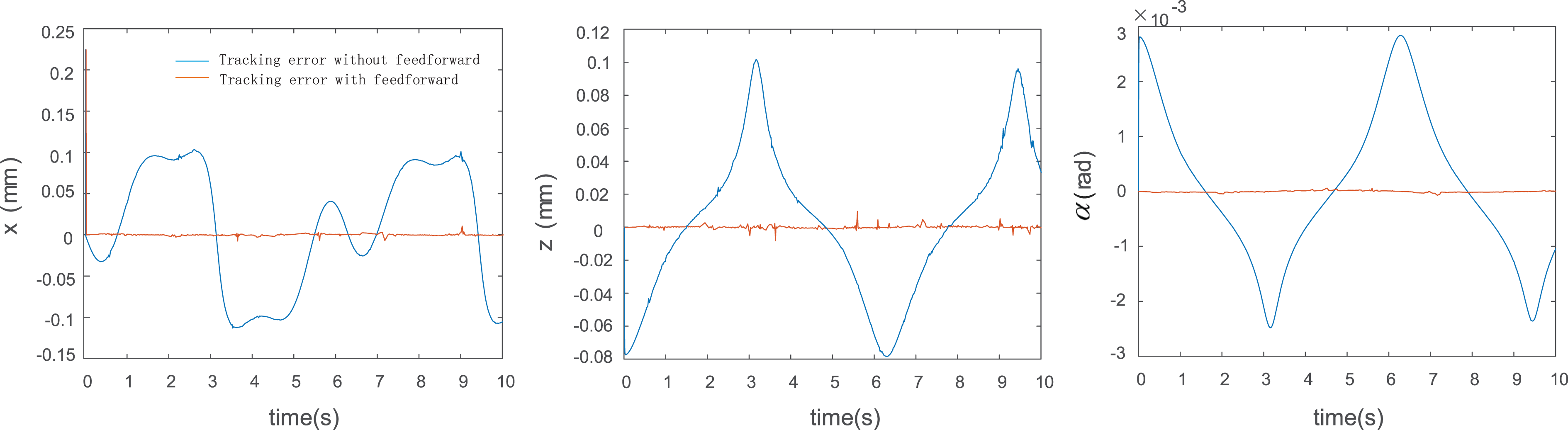
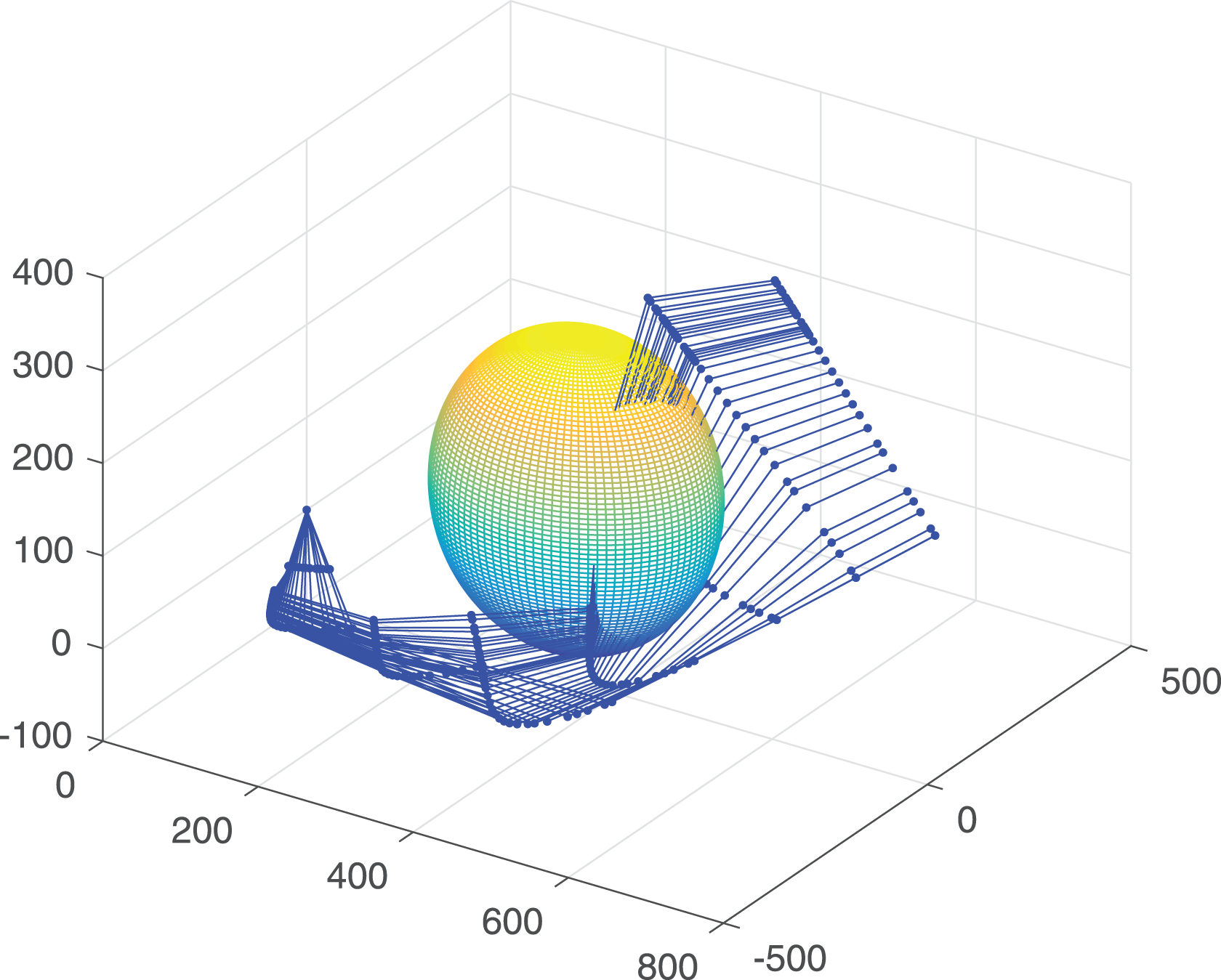
Obstacle avoidance simulations were conducted under the premise of the obstacle being simplified into a sphere. Considering the obstacle as a sphere, ensured that only a pair of the nearest points existed between the obstacle and each joint of the manipulator for every moment. As shown in Figure 16, the shortest distance d can be expressed as ³¹

$d=\Vert Q-S\Vert -R-r$

28

where Q is the sphere center, and S is the shortest point on line oo. And the direction of repulsive force ${\overrightarrow{F}}_{\text{rep}}$ also can be presented as

$\overrightarrow{u}=\frac{1}{\Vert S-Q\Vert }\left[\begin{array}{c}{S}_x-Q_x\\ S_y-Q_y\\ S_z-Q_z\\ 0\\ 0\\ 0\end{array}\right]$

29

Figure 16.

Simplified schematic of collision detection.

In this case, repulsive force ${\overrightarrow{F}}_{\text{rep}}$ can be easily obtained with the manipulator approaching the obstacle. When the manipulator performed the task of drawing a circle as mentioned above, a spherical obstacle was placed in its working space. The coordinates of sphere center Q was (500, 0, 250), and r and R were 68.5 mm and 100 mm, respectively.

In this regard, collision detection could be further simplified. The joint could be seen as line segment oo, and the radius of the spherical obstacle should be the sum of the original obstacle radius R and joint radius r; therefore, the radius of the spherical obstacle can be written as $R_{\text{sum}}=r+R=168.5$ .

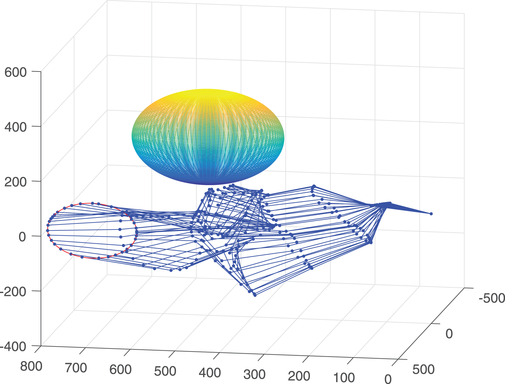
Without obstacle avoidance, the configurations of the 9-DOF manipulator are shown in Figure 17. Additionally, the closest distance between the joint and the obstacle is shown in Figure 18. Because the minimum distance was less than zero for some time, it is obvious that the manipulator collided with the obstacle. To design an obstacle avoidance algorithm in this case, d₀ and K_rep were, respectively, considered as $d_0=30\hspace{0.17em}\text{mm}$ and $K_{\text{rep}}=1$ . The simulation results are shown in Figures 19 and 20, and the effectiveness of the obstacle avoidance algorithm was verified obviously according to these two figures. The obstacle avoidance algorithm proposed in this article can not only achieve obstacle avoidance for single obstacle but also achieve obstacle avoidance with multiple obstacles. It is proved by adding an identical sphere obstacle at point $o(500,0,-400)$ as shown in Figures 21 and 22. From Figures 23 and 24, the presented algorithm also succeeded in achieving obstacle avoidance in the position control process.

Figure 17.

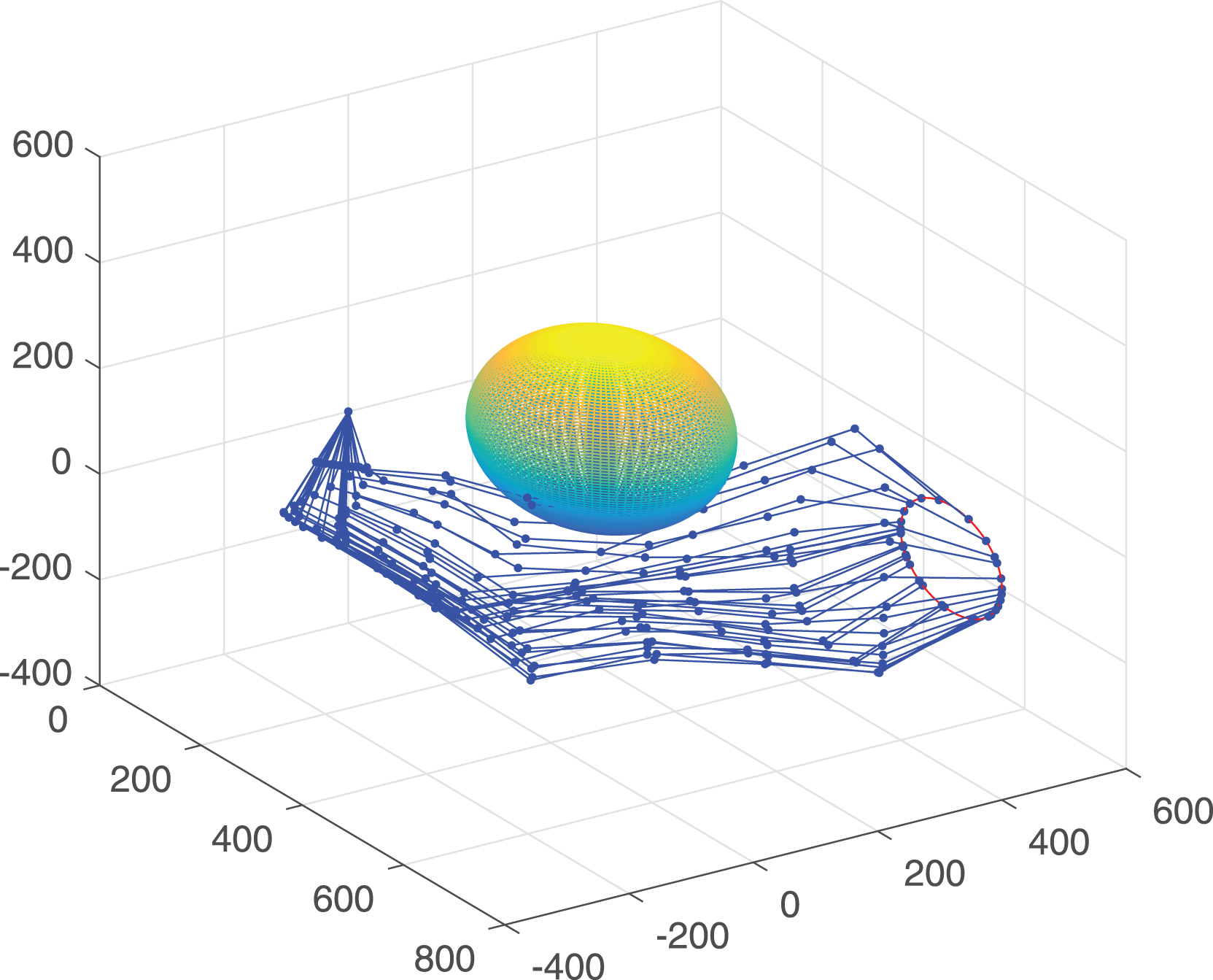
Configuration profiles of the manipulator moving along a continuous trajectory without obstacle avoidance.

Figure 18.

Closest distance between the joint and obstacle without obstacle avoidance.

Figure 19.

Configuration profiles of the manipulator moving along a continuous trajectory with obstacle avoidance.

Figure 20.

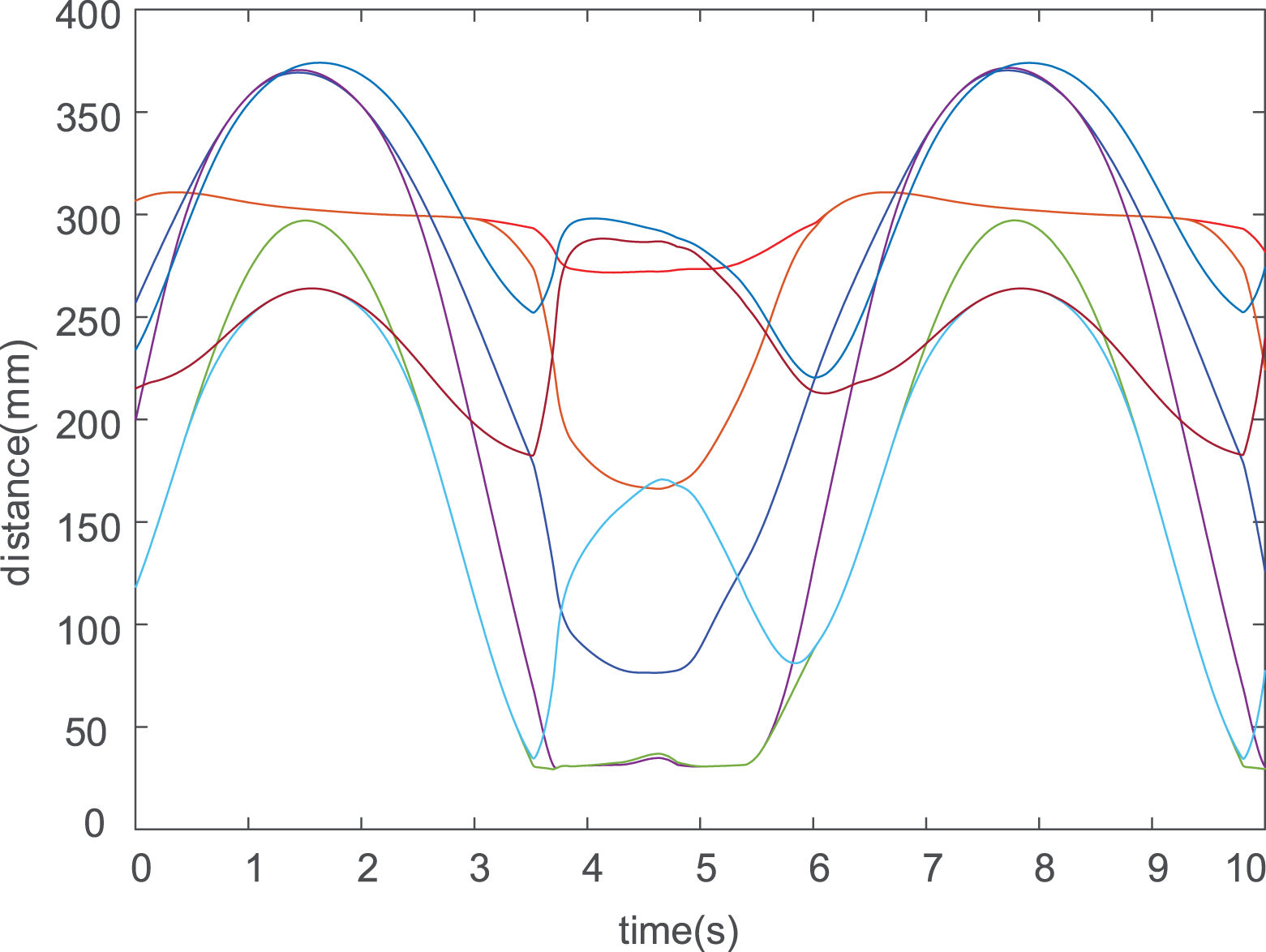
Closest distance between the joint and obstacle with obstacle avoidance.

Figure 21.

Configuration profiles of the manipulator moving along a continuous trajectory without obstacle avoidance for multiple obstacles.

Figure 22.

Configuration profiles of the manipulator moving along a continuous trajectory without obstacle avoidance for multiple obstacles.

Figure 23.

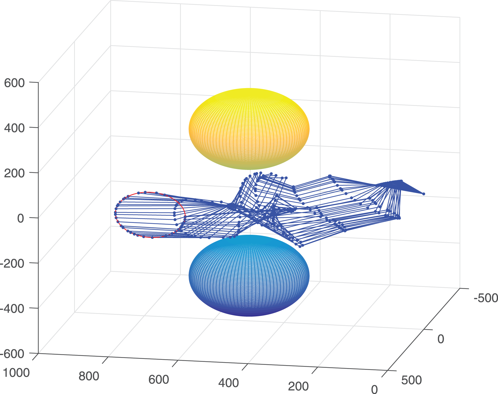
Configuration profiles in position control without obstacle avoidance.

Figure 24.

Configuration profiles in position control with obstacle avoidance.

Conclusions

By introducing the artificial potential field model, the main task, trajectory planning, and the subtasks, obstacle avoidance and joint limit avoidance, both can be donated as fictitious forces acting on end-effector or joint. The forces can be resolved to joint velocities to drive the manipulator. This make the complicated task such as obstacle avoidance and joint limit avoidance easier and the control process more clearly, because we only need to control the joint velocities.

The trajectory planned using the proposed method in this article could meet the joint velocity limits and angle limits. And its tracking error was less than 10–3 mm for translational components and less than 10–5 rad for rotational components. In the case of position control, the tracking error was smaller. The obstacle avoidance algorithm proposed could ensure that the manipulator avoided the obstacle when its end-effector performed certain tasks not only for single obstacle but also for multiple obstacles. The correctness and superiority of the trajectory planning algorithm and obstacle avoidance algorithm based on the artificial potential field were verified by simulation results. Obstacle avoidance was achieved through defining the relation between the fictitious force and the distance of the nearest points on the obstacle and the joint. So we could ignore the specific shape of the obstacle, as long as we could get the information of the obstacle surface point, the real-time obstacle avoidance could be achieved. In the future work, we can combine obstacle avoidance algorithms with vision to make it more widely used.