Sage Journals: Discover world-class research

Abstract

We present a deliberative trajectory planning method to avoid collisions with traffic vessels. It also plans traversal across wavefields generated by these vessels and minimizes the risk of failure. Our method searches over a state-space consisting of pose and time. And, it produces collision-free and minimum-risk trajectory. It uses a lookup table to account for motion uncertainty and failure risk. We also present speed-up techniques to increase performance. Our wave-aware planner produces plans that (1) have shorter execution times and safer when compared to previously developed reactive planning schemes and (2) comply with user-defined wave-traversal constraints and Collision Regulations (COLREGs)

Keywords

Trajectory planning obstacle avoidance dynamic obstacles waves perception uncertainty motion uncertainty

Introduction

Automated trajectory planning is a prerequisite for realizing autonomous unmanned vehicles. Collision avoidance with static and dynamic obstacles under perception uncertainty are basic requirements for generating useful trajectories. The focus of this article is a framework for deliberative trajectory planning in the presence of large semipermeable dynamic obstacles and motion uncertainty. Typically, trajectory planning for unmanned vehicles is decoupled into two parts. First, a path planning problem is solved to obtain a tentative path, ignoring dynamic obstacles. Then, a motion planning problem is solved, this time considering dynamic obstacles, using the tentative path as a reference to yield a final trajectory. The motion planning problem is conventionally solved using reactive planning approaches like generalized velocity obstacles¹ and velocity tuning.^2
–4 These methods work well when the dynamic obstacles are small, and the introduction of these dynamic obstacles does not introduce drastic differences between the true optimal path and the tentative path. Thus, in the case of small dynamic obstacles, a reactively planned trajectory is likely to be close to the true optimal trajectory while following a tentative path computed while ignoring small dynamic obstacles. However, in the case of large dynamic obstacles, it is generally likely for reactively planned trajectories to be highly suboptimal. For instance, on the one hand, reactively avoiding (i.e. going around) large dynamic obstacles may introduce unnecessary slowdowns and increase execution time. On the other hand, punching through semipermeable dynamic obstacles may decrease execution time but increase the risk of failure and collisions. Therefore, handling large semipermeable dynamic obstacles requires deliberative planning that can carefully balance the competing priorities (i.e. reduce execution time, reduce failure/collision rate). For example, reducing failure/collision rate should be the first priority. When it is possible to have zero failures/collisions, reducing execution time is the next priority. In some situations such as those that arise in the marine robotics domain,⁵ navigation around or through large permeable dynamic obstacles is required (Figure 1).

Figure 1.

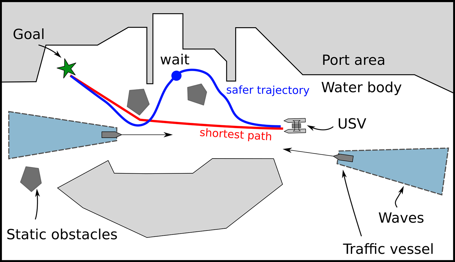
Handling large dynamic obstacles requires deliberative planning.

The wavefield generated by a marine vessel is a good example of a large semipermeable dynamic obstacle which can either be traversed or be avoided altogether. In a majority of practical scenarios, unmanned ground vehicles exhibit significantly less motion uncertainty compared to unmanned surface vehicles. Trajectory planning for unmanned ground vehicles is a well-studied problem and in the recent years, significant progress has been made in solving it using a wide variety of methods such as graph search,⁶ stochastic tree search,^7,8 Markov decision processes (MDPs), and optimal control.^9,10 Graph search methods like state lattice search are popular global planning methods due to optimality guarantees and efficiency in large environments. Unmanned surface vehicles exhibit more motion uncertainty due to significant external disturbances like waves and winds.¹¹ Collision avoidance is more challenging under these circumstances and it involves not only staying a safe distance from static obstacles and dynamic obstacles but also following COLREGs. COLREGs is a set of maritime navigation rules set by the International Maritime Organization (IMO) to minimize collisions and confusion among marine vessels. The effects of motion uncertainty are pronounced in smaller Unmanned Surface Vehicles (USVs) as they are more susceptible to wave disturbances. An MDP framework can rigorously handle motion uncertainty for environments with static obstacles. It requires a state transition model of the USV. A state transition model to account for wave disturbances is developed in Thakur et al.¹² for use in path planning amid static obstacles. In addition to ambient sea waves, wavefields generated by the motion of dynamic obstacles over the sea create yet another source of motion uncertainty and adds to the number of failure modes. The wavefield induces external disturbances that vary both spatially and temporally. Trajectory planning for USVs in the presence of dynamic obstacles needs to consider a state vector that includes position, orientation, velocity, and time. For time-varying environments, the regular MDP can be converted to a time-extended MDP.¹³ Time-extended MDP over high-dimensional state spaces are complex and computationally prohibitive.^14,15 On the other hand, performing a search over a lattice of motion primitives requires careful collision risk assessment and heuristics tuned for dealing with dynamic obstacles in the presence of significant motion uncertainty. Large-scale partially observable Markov decision processes (POMDPs) can be approximately solved only in a reactive online fashion using methods developed in the literature.^16,17

This article builds on the work in Rajendran et al.¹⁸ As in Rajendran et al.,¹⁸ we only focus on the environmental disturbance caused by wavefields, and hence, the effects of wind and water currents are not considered. In Rajendran et al.,¹⁸ dynamic obstacle heuristics (DOHs) was used requiring extensive precomputation for traffic vessels of different sizes and velocities using off-line simulations. This needs to be done for a planning scenario before the search can be performed. Computing lookup tables takes considerable amount of time. Therefore, this method cannot be used in practice in new scenarios. The method described in this article overcomes that limitation and uses online heuristics instead of precomputed lookup tables. Both methods lead to almost identical paths.

The new contributions of this article are the following. (1) We adapt the idea of space–time heuristics¹⁹ to overcome the limitations of DOH used in our exploratory work. We also incorporate COLREGs rules into it to solve more difficult problems involving many dynamic obstacles. (2) We investigate the behavior of our method in four new maps that capture the types of environments the USV may be exposed to. (3) We characterize the behavior of our method under different operating conditions involving varying perception uncertainty, varying number of dynamic obstacles, and varying wavefield parameters.

Related work

Trajectory planning

Precomputed state-transition probabilities over differing sea states are used in Svec et al.¹¹ to handle motion uncertainty. Incorporating perception uncertainty turns MDPs into POMDPs. In Agha-mohammadi et al.,²⁰ the probabilistic road map idea is extended for belief spaces using MDPs and feedback controllers. Feedback controllers are designed to drive the agent into a sampled state in belief space called a Feedback Information Road Map (FIRM) node. Then, through the use of a precomputed policy for the MDP over FIRM nodes, a sequence of controllers that drive the agent from the initial state to the final state is obtained. This way POMDPs become computationally tractable for problems of larger scale involving only static obstacles. However, it is hard to augment these methods to work in domains with spatiotemporal disturbances. In Blackmore et al.,²¹ chance constraints are used in the context of static obstacle avoidance, guaranteeing prespecified failure probability bounds. Belief-space (pose × covariance space) search is used in static obstacle environments to incorporate motion uncertainty and generate plans that expedite arrival time and minimize final pose error covariance.^22,23 These works do not include dynamic obstacles. Terrain variation causes trajectory tracking error. The error characteristics of the controller are considered in the planning method proposed in Mellinger and Kumar²⁴ where tracking error is modeled as a function of terrain. The probability of successful navigation through the terrain is incorporated into the cost function. We take inspiration from Mellinger and Kumar²⁴ and introduce the notion of time-varying terrain. We also account for risk of failure through a robot-reliability model.²⁵ We also use methods in Greytak and Hover²⁶ to model trajectory tracking uncertainty and utilize low-level trajectory tracking error characteristics.

Trajectory and wave prediction

Accurate prediction of trajectories of moving obstacles is a fundamental requirement for deliberative trajectory planning. Several threads of research work are in progress to provide predictions. In the marine domain, automatic identification system (AIS) data²⁷ can be used for coarse grained trajectory prediction. AIS is susceptible to communication interruptions.²⁸ However, when it is used in conjunction with Gaussian Process Regression (GPR) based trajectory prediction methods,^8,29
–31 it can produce good estimates for long-term planning purposes.³² Waves generated by moving vessels can be forecast up to 180 s into the future using radar systems.^33,34 We assume such a system is available in the sensor suite to aid deliberative planning.

Preliminaries and problem formulation

Vehicle model

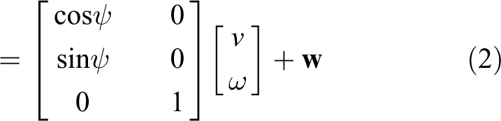
For trajectory planning purposes, we use a simplified kinematic vehicle model to describe the motion of the USV

\dot{x} = f (x, u, w)

= [\begin{matrix} cos ψ & 0 \\ sin ψ & 0 \\ 0 & 1 \end{matrix}] [\begin{matrix} v \\ ω \end{matrix}] + w

The USV pose is $x = (x, y, ψ)^{T}$ where x and y denote the position in North-East-Down coordinates, ψ denotes heading with respect to north. The USV control variables are $u = (v, ω)^{T}$ and w is a zero-mean random process noise capturing the effects of environmental disturbances. A state s is defined by the tuple $(x, y, ψ, t, p_{s})$ encoding the USV pose, the time stamp, and probability of being operational up to a time duration t from the start time. A motion goal is a tuple $MG = (x_{f}, y_{f}, ψ_{f}, t_{f})$ encoding a pose $(x_{f}, y_{f}, ψ_{f})$ to be reached at time instant t_f . Given an initial state x _i and a final state $x_{f} = (x_{f}, y_{f}, ψ_{f})^{T}$ specified by the motion goal MG, and letting w=0, a nominal trajectory $\overset{⌣}{x} (t)$ satisfying $\overset{⌣}{x} (t_{i}) = x_{i}, \overset{⌣}{x} (t_{f}) = x_{f}$ can be computed using trajectory generation methods.^9,
35 We assume that the underlying trajectory tracking controller of the USV will achieve the target pose x_f by the time deadline t_f . In our work, we use Dubins curves³⁶ as the optimal trajectory between motion goals. We also use only 70% of the maximum allowable USV speed as the controller may need to saturate the throttle occasionally to make up for lost time while rejecting disturbances. A motion goal set ${MGS}_{r, n_{dirs}} (s)$ is a set of motion goals that are a distance of r units away relative to a particular state s and directed at $n_{dirs}$ different angles. Each of the motion goals is given a label l corresponding to its direction from s. Thus, ${MGS}_{r, n_{dirs}} (s) = {{MG}_{l}} \cup {MG}_{O}$ , where $l = k \times 360 / n_{dirs}, k \in [0, n_{dirs} - 1]$ . The label O indicates a wait action of duration $Δ t_{wait}$ at the same pose. We assume a station-keeping controller³⁷ is active for the duration of the wait action. Figure 2 shows an example of a labeled motion goal set ${MGS}_{r = 30 m, n_{dirs} = 8} (s)$ where $s = (x = 0, y = 0, ψ = 0, t = 0)$ . r is adapted to have multiple resolutions depending on how congested the local region is. This allows for high-resolution motion goals in areas which are difficult.

Figure 2.

Motion goal set with $r = 30 m$ containing $n_{dir} = 8$ motion goals (in blue) directed toward cardinal and intercardinal directions. Eight optimal trajectories (in red) from $(x = 0, y = 0, ψ = 0, t = 0)$ to each of the motion goals is shown. A ninth motion goal labeled O is also shown which corresponds to a wait-action of duration $Δ t_{wait}$ . The trajectories start with ψ=0 and end at the heading angle corresponding to the cardinal directions.

Traffic vessel profiles

A traffic vessel profile (TVP) is a collection describing the geometry and state of a traffic vessel underway. These data are generated by a trajectory prediction system.³¹ A typical traffic vessel profile TVP _i made up of the following quantities: (i) predicted trajectory ${\bar{p}}_{i} (t)$ , (ii) instantaneous position covariance matrix $Σ_{i} (t)$ , (iii) vessel zones ${Z_{k}}_{k = 1}^{3}$ where each Z_k is an ellipse attached to and defined in the body frame of the vessel (see Figure 3). The vessel zones move in unison with the traffic vessels. Vessel zone 1 is a region with 100% probability of failure. Vessel zone 2 and 3 denote regions where significant wave disturbances are expected. These zones also specify the local wave front direction in that region. We assume that waves outside the zones 1, 2, and 3 do not affect the USV. The sizes of these vessel zones are application-dependent. In this work, the length of zone 1 is fixed to three boat-lengths long, and it can be made longer for vessels traveling at a higher relative speed compared the USV. The length of zones 2 and 3 have been chosen based on the attenuation of the wavefield and where the wavefield poses no danger to the USV. A set of TVPs is denoted by $TVPS = {{TVP}_{k}}_{k = 1}^{n_{t v}}$ .

Figure 3.

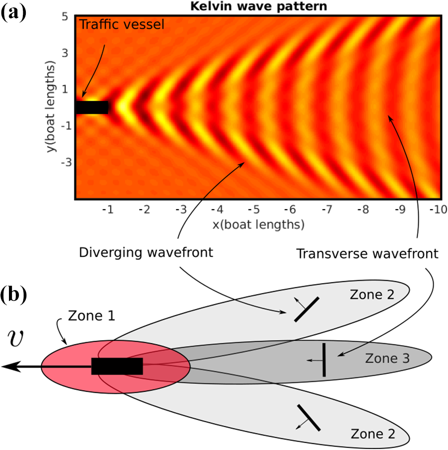
(a) A wave pattern (Kelvin wave) for a traffic vessel moving westward, operating at hull Froude number 0.5 and waterline boat length 10 m. Crests are shown in yellow and troughs are shown in red. Two local wave fronts near two instances of the USV are labeled 1 and 2, (b) a simplified wave pattern consisting of zones with different local wave fronts.

Environmental disturbances

We assume environmental disturbances are specified parametrically through a parameter vector defined for each state in the state space as in Figure 4. For example, at point D, $γ_{D} = {seastate = calm, nearvessel = false}$ where sea states are defined as in the Douglas sea scale.³⁸ Point C lies in a static obstacle region and hence, $γ_{C} = {invalid = true}$ is left undefined and handled as a special case. Whenever a traffic vessel passes through a point, for example, point A at a certain time t, the parameter vector is updated as $γ_{A} = {seastate = calm, nearvessel = true, wavezone = Z_{2}$ }. Similarly, at point B, $γ_{B} = {seastate = rough, nearvessel = true, wavezone = Z_{3}}$ . In both cases A and B, the local wave amplitude and wave direction can be determined given the wave zone and the pose of the traffic vessel at t. The field near vessel in γ indicates that the point is in some zone of some traffic vessel.

Figure 4.

An illustration showing how parameter vector γ is defined over a trajectory at a few characteristic query points A, B, C, and D.

In this work, TVPs and environmental disturbances are modeled with the help of basic wave models. In practice, the wave interaction is more complex and estimation of wave parameters is required. With recent advances of computer vision and deep learning, it is possible to construct a method of wave parameter estimation from vision. This method does not have to be very accurate for use in a failure assessment module.

Failure model

We seek to model failure probabilities using a robot reliability model.²⁵ The probability that a robot remains functional up to time t is given by $p_{s} (t) = e^{- t / M}$ where M is the mean-time-between-failures (MTBF), which is estimated as

M = \frac{Total observation duration}{Number of failures during observation}

the ratio of number of failures to the total number of attempts within an observation time window. Developing a precise model of the failure (i.e. capsize) of the USV in varying sea-states and waves is difficult. It involves allowing the robot to fail in the process of counting the number of failures within an observation time window. This is not practical. A safer alternative is to measure how close to failure the robot got to when exposed to a certain local disturbance. In this work, a local disturbance is described parametrically as the tuple consisting of sea-state and proximity to a vessel. Two sea-states are considered calm (undisturbed waters) and rough (choppy waters due to wind conditions/multiple traffic vessels). And, proximity to vessel is a Boolean flag that is determined by whether the USV happens to be in any of the wavezones around the traffic vessel (see Figure 5). If the USV is in proximity to a vessel, then the wavezone is also part of the local disturbance parameter. USVs typically have certain design limits such as roll limits or pitch limits. We define a failure event as an event when any of these design limits is exceeded. Thus, given a set of trajectory samples ${s_{k} (t)}_{k = 1}^{n_{k}}$ as in Appendix A of duration t₁. For each trajectory sample, we count the number of failure events during t₁. With failure events labeled and counted, compute M as in equation (3) for each trajectory sample. We aggregate the MTBF over trajectory samples for each combination of local disturbance parameter γ. In this way, a lookup table that is indexed by γ can be generated (see Table 2). Once MTBF estimates are computed for an USV operating in different local disturbance parameters, it can later be used in the robot reliability model to compute failure probabilities.

Figure 5.

Determining wave incidence angle and relative position from a traffic vessel.

Table 1.

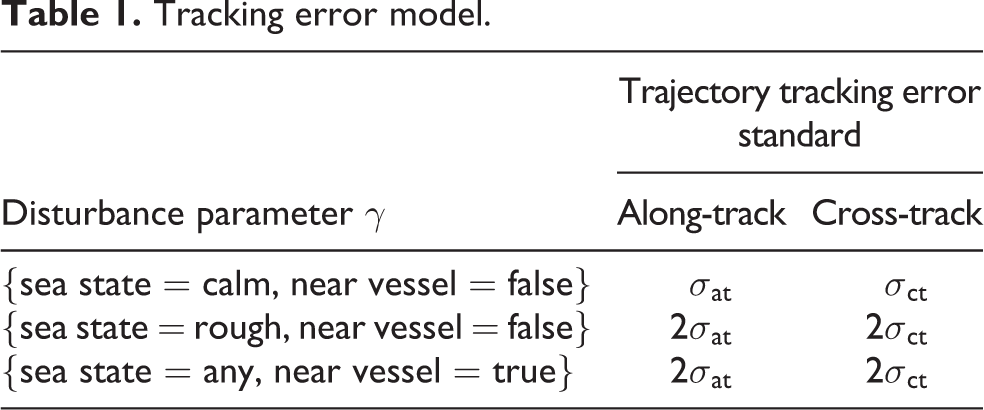
Tracking error model.

	Trajectory tracking error standard
Disturbance parameter γ	Along-track	Cross-track
{sea state = calm, near vessel = false}	σ _at	σ _ct
{sea state = rough, near vessel = false}	2σ_at	2σ_ct
{sea state = any, near vessel = true}	2σ_at	2σ_ct

Table 2.

Mean-time-between-failure (MTBF) model.

Disturbance parameter γ	MTBF
{sea state = calm, near vessel = false}	M_c
{sea state = rough, near vessel = true/false}	M_r
{sea state = calm, near vessel = true, wave zone = $Z^{'}$ }	M_t
{invalid = true}	0

Problem formulation

Given: (i) Initial state $s_{i} = (x_{i}, y_{i}, ψ_{i}, t_{i}, p_{s} = 1)$ , (ii) a region G around the goal state $s_{f} = (x_{f}, y_{f}, ψ_{f})$ , (iii) a set of TVPs, $TVPS = {{TVP}_{k}}_{k = 1}^{n_{v}}$ , sensed by the perception system, (iv) a set of static obstacles defined by a set of polygons SO.

Compute: A sequence of states ${s_{k}}_{k = 0}^{p}$ such that (i) $s_{0} = s_{i}$ , (ii) $s_{p} \in G$ , (iii) the trajectory is COLREGs compliant, (iv) probability of success p_s at $s_{p}$ is maximized, (v) expected time of execution is minimized.

Approach

The problem is an implicit graph search problem. We use the Theta* graph search algorithm³⁹ to solve it. We describe the essential aspects of the Theta* graph search implementation.

Node expansion and cost functions

A node n is a tuple defined as $n = {s, g, h, f}$ where g is the cost-to-come, h is the cost-to-go, f is the total cost ( $f = g + h$ ), s is the state. An initial node n_i is constructed as $n_{i} = {s_{i},0, h (s_{i}, s_{f}),0 + h (s_{i}, s_{f})}$ . When a parent node n_p is visited, a set of child nodes ${n_{c, k}}_{k = 1}^{N_{c}}$ that contain with states corresponding to the nearby motion goals are assigned. Here N_c is the total number of child nodes expanded for n_p . Each of the child nodes also contains the reference trajectory $\overset{⌣}{x} (s_{p}, s_{c, k})$ composed of the Dubins curve linking the parent state to the child state. During execution, there is motion uncertainty as the controller tracks the reference trajectory. This uncertainty is handled while evaluating the cost function. To describe the cost function, we focus on the expansion of an arbitrary parent node n_p resulting in a child node n_c ending in the state $s_{c}$ as in Figure 6. Let us assume the reference trajectory $\overset{⌣}{x} (s_{p}, s_{c})$ starts at $t = t_{p}$ and ends at $t = t_{c}$ . To evaluate the cost function, the reference trajectory must be discretized into temporal segments. Performing regular discretization, we obtain a sequence of time samples $TS = {t_{q}}_{q = 1}^{n_{t s}}$ where $t_{q} \in [t_{p}, t_{c}]$ , $t_{q + 1} - t_{q} = Δ t$ . Suppose that for a $\overset{⌣}{t} \in TS$ , the reference trajectory puts the USV state at $\overset{⌣}{s}$ with the 2D position being $\overset{⌣}{p}$ and time being $\overset{⌣}{t}$ . And, similarly, all of traffic vessels are moved to $\overset{⌣}{t}$ on their mean predicted trajectory. The uncertainty in the predicted trajectory will be considered in Cost assessment. Having moved the traffic vessels to their positions in the environment map, the local disturbance vector $\overset{⌣}{γ}$ is obtained by looking up $\overset{⌣}{p}$ on the environment map and identifying which of the characteristic scenarios apply (see Figure 4). We will now see how $\overset{⌣}{γ}$ is used in the trajectory evaluation process.

Figure 6.

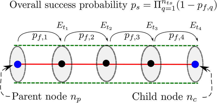
Collision cost calculation for a trajectory between a parent node and a child node.

Obtaining tracking error and failure model parameters

Local environmental conditions (such as local sea state) and being in the vicinity of a moving vessel affect the trajectory tracking performance of the USV as it moves along a reference trajectory. These conditions are encoded into $\overset{⌣}{γ}$ (Figure 4) and can be used to obtain tracking error and failure model parameters. If the USV were to be controlled in an open-loop configuration, the trajectory tracking error would build up over time. However, in the presence of a low-level stabilizing feedback controller, the tracking error can be bounded within an envelope around the reference trajectory.⁴⁰ Environmental disturbances and controller can be extensively studied off-line by either using Monte Carlo simulations. This way the various realizations of the transition trajectories can be obtained.¹² These trajectories can also be obtained by empirically evaluating them in real scenarios. With either approach, the goal is to characterize the USV motion as it is commanded to move in a straight line from an initial state s₀ toward a motion goal under parameterized disturbances in the environment. Appendix A outlines a simple procedure to identify tracking error parameters. We seek to model the tracking error and the probability of successful navigation along the reference trajectory as a function of the local disturbance parameter vector $\overset{⌣}{γ}$ . The tracking error can be characterized by observing cross- and along-track errors (see Figure 7). The cross-track error at any point in time is the deviation in a direction normal to the reference trajectory (i.e. lateral deviation). The along-track error at any point in time is the difference in the track-projected current position and the target point on the trajectory (i.e. lag or overshoot). The probability of successful navigation can be characterized by measuring MTBF under different conditions. To this end, we conducted preliminary experiments with a 16-foot Wave Adaptive Modular Vehicle (WAM-V) USV³⁷ in the Stranahan River, near Dania Beach, Florida. We chose the WAM-V platform due to its robustness under wave action. We could safely perform the physical experiments while not risking the total loss of the robot. However, this work is applicable to platforms that are not specifically designed to withstand waves that may cause hull damage. We collected data using wave gauges and the navigation sensors (Inertial Measurement Unit (IMU), GPS, Compass) of the USV (Figure 8) and studied the effect of the waves generated by a traffic vessel on the WAM-V. Due to the difficulties of controlling sea-state, only two states calm and rough were considered. Calm condition refers to a situation when water level across the test area is roughly constant, and no wind effects are seen on the surface of the water. Rough condition refers to a situation when water levels are changing due to interacting waves generated by passing traffic vessels and wind. In both conditions, the USV was made to traverse a 20 m linear path $10$ times and the cross-track σ_ct and along-track σ_ct error standard deviation in the tracked trajectory was used to populate Table 1. Similarly, in both sea-state conditions, the pitch and roll angles recorded and the procedure in Determining MTBF is used to compute M_r and M_c in Table 2. M_t is not generated using physical experiments instead we use a surrogate model defined by equation (4). In a very rough sea-state, the data from IMU are likely to be noisy and other sensing modalities might be needed for producing better estimates. Since we performed experiments in a water channel, our experiments were shielded from disturbances and did not experience noisy IMU measurements and we were able to observe roughly sinusoidal variations as the waves passed by. Tables 1 and 2 are indexed by the local disturbance parameters in γ and they are briefly explained below.

Figure 7.

(a) Error envelope of trajectory tracking defined by σ_ct and σ_at for a trajectory starting at $p_{q} = (0, 0, 0)$ , $t_{q} = 0$ and reaching east under a particular sea state γ, (b) the 3σ error ellipse at an intermediate time $\bar{t}$ along the nominal trajectory.

Figure 8.

Wavefield experiment setup.

Determining tracking error parameters

As for the tracking error model, when the query state lies over calm waters and is not in the vicinity of any traffic vessel, we use nominal values for tracking error parameters. Otherwise, the tracking error parameters are doubled.

Determining MTBF

Since traffic-free calm waters are very safe, $M_{c} = \infty$ . Since rough waters are not safe regardless of traffic, $M_{r} = 600$ . Determining MTBF over calm waters near traffic vessels involves determining the angles between the waves and the heading of the USV as shown in Figure 5. If the query state is located within any zone of the traffic vessels, we determine the relative position p_d from the center of the traffic vessel and the incidence angle θ_i between the USV heading and the wave direction of zone Z' (see Figure 5). p_d is calculated in the body-fixed coordinates of the traffic vessel and $d = [\begin{matrix} 1 & 0 \end{matrix}] p_{d}$ . Sailors typically prefer the incidence angle to be around 45, reducing the risk of broadside rolling as well as pitchpoling.⁴¹ Adhering to this notion, we use the following assignment for MTBF

α = \{\begin{matrix} 1.0, & - \frac{π}{8} \leq θ_{i} - \frac{π}{4} \leq \frac{π}{8} \\ 0.25, & otherwise, \end{matrix}

M_{t} = \{\begin{matrix} 0, & p_{d} \in Z_{1} \\ α M_{Z^{'}} d / L_{z}, & \exists k \in {2, 3}, p_{d} \in Z_{k} \\ M_{c}, & otherwise . \end{matrix}

Here $M_{Z^{'}}$ is the MTBF value associated with the zone Z' and is defined as $M_{Z_{1}} = 0$ , $M_{Z_{2}} = 1000$ , $M_{Z_{3}} = 3000$ . And, L_z is the maximum trailing length of the traffic vessel zones.

In this work, the MTBF model was generated using a combination of simulation and physical experiments. These were done in an off-line manner. In future, these can be performed in an online manner as well. We envision that it will work in the following manner. Initially, we assume a conservative MTBF model. Using this conservative MTBF model, the USV can navigate safely. And, based on an explore-exploit tradeoff, we can explore unknown wave conditions and update MTBF model appropriately using a Bayesian inferencing scheme. This will enable exploring new wave conditions while safely updating the MTBF model parameters.

Cost assessment

Having determined the tracking error and the MTBF parameters using $\overset{⌣}{γ}$ , we proceed to evaluate the cost function along the reference trajectory $\overset{⌣}{x} (s_{p}, s_{c})$ . Tracking error parameters σ_at and σ_ct encode the deviation along the path and the normal deviation from the position $\overset{⌣}{p}$ , respectively (see Figure 7). Thus, the actual position p of the USV at $\overset{⌣}{t}$ is given by

p = \overset{⌣}{p} + c N [\overset{⌣}{p}] + a T [\overset{⌣}{p}]

where $c \sim N (0, σ_{c t})$ and $a \sim N (0, σ_{a t})$ . $N [\overset{⌣}{p}]$ and $T [\overset{⌣}{p}]$ are the normal and tangent unit vectors at $\overset{⌣}{p}$ . An ellipse $E_{\overset{⌣}{t}}$ centered at $\overset{⌣}{p}$ and aligned to the tangent direction $T [\overset{⌣}{p}]$ and normal direction $N [\overset{⌣}{p}]$ with axis lengths $6 σ_{at}$ and 6σ_ct describes a 99.7% confidence region within which the USV can be expected to be at $t = \overset{⌣}{t}$ (99.7% comes from the 68-95-99.7 empirical rule associated with the normal distribution).

For each ellipse $E_{t_{q}}$ , the probability of failure $p_{f, q}$ is computed as

p_{f, q} = 1 - exp (- \frac{Δ t}{M_{q}})

where M_q is computed by averaging the MTBF values over a uniform set of points in $E_{t_{q}}$ . More specifically, these MTBF values are computed by looking up each point in Γ and then using Table 2 to find the MTBF. Assuming independence of the failure events, the final probability of success for executing $\overset{⌣}{x} (s_{p}, s_{c})$ is given by $p_{s} = Π_{q = 1}^{n_{t s}} (1 - p_{f, q})$ .

Thus, the probability of success imparted to the child state is $p_{s} (n_{c}) : = p_{s} (n_{p}) \times p_{s}$ where $p_{s} (n_{p})$ and $p_{s} (n_{c})$ are the probabilities of success of the parent and child states, respectively. The child node n_c is then assigned a cost-to-come $g (n_{c})$ where

g (n_{c}) : = g (n_{p}) + (1 - ω_{f}) c_{t} - ω_{f} F_{f} log (p_{s}) + c_{c} F_{c}

the time cost is $c_{t} = t_{c} - t_{p}$ , F_f is a large constant with units of time discouraging risky motion causing failure, and F_c is a large constant with units of time discouraging moves that violate COLREGs. Parameter $c_{c} \in {0, 1}$ encodes the violation of COLREGs computed using.^42,43 Parameter $ω_{f} \in [0, 1]$ is a user defined weight parameter.

Accounting for perception uncertainty

To account for the perception uncertainty in the measurement of the TVPs, a Monte Carlo sampling scheme⁴⁴ is utilized. The Monte Carlo sampling approach is used as it is a general method and amenable to parallelization. In the previous section, $\overset{⌣}{γ}$ was computed using only the mean position of traffic vessels at $\overset{⌣}{t}$ . However, to account for uncertainty, covariance information needs to be used. We pick one TVP, $T V P_{i} \in T V P S$ , to illustrate the process. A set of possible instantaneous positions ${PS}_{i} = {p_{k}}_{k = 1}^{n_{ps}}$ is sampled from the distribution $N ({\bar{p}}_{i} (\overset{⌣}{t}), Σ_{i} (\overset{⌣}{t}))$ . We move the traffic vessel to each possible position $p_{k} \in {PS}_{i}$ and then look up γ_k as in Figure 4. We compute the corresponding M_k using Table 2 and Figure 5. Finally, we compute the average M over all the computed M_k . This average M is used in place of the original MTBF in equation (7).

Speed-up techniques

We describe some techniques to improve the search performance.

Static obstacle heuristics

The cost function includes the time duration of moving from one position to another (i.e. c_t ). And, static obstacles do not move between planning cycles. In such a scenario, a time-to-goal map (also known as arrival time map) is beneficial. This map is termed Static Obstacle Heuristic (SOH) and it stores the lower bound on the time cost of going from any position in the workspace to the goal position g. This map is computed using the fast marching method (FMM) to approximately solve an Eikonal equation.^45,46 The level sets of the solution of the Eikonal equation correspond to the frontiers of a wave emanating from the goal position. The speed of the wave is set to the maximum speed of the USV. As the frontier (i.e. the open set in Dijkstra’s algorithm) bends around corners, the time-to-goal estimate is more informative than the naive Euclidean distance-based estimate. The raw time-to-goal values given by the FMM are naturally not admissible unless they are scaled down by a factor that depends on the discretization used in computing the map.⁶ After the appropriate scaling is applied, each cell in this map contains an underestimate of the time to reach the goal from that cell location. This value is used to compute an estimate of c_t to be accumulated until the goal is reached. For a given query position s, a heuristic value $h_{s} (s, g)$ is looked up from the SOH.

Space–time exploration heuristics

Developing admissible heuristics to handle dynamic and static obstacles is challenging and can often be just as hard as the original problem. However, by relaxing the original problem, effective heuristics can be generated. We follow Chen et al.¹⁹ and drop to 3D configuration space by excluding ψ (i.e. we use only $x - y - t$ space) to generate a heuristic trajectory using a point robot kinematic model (relaxed version of the USV kinematic model) from initial state s_i to the goal region G. Maximum speed v_max of the point robot is the same as that of the USV. We also ignore zones 2 and 3 of traffic vessels such that only zone 1 is considered as a dynamic obstacle. In other words, for the purpose of heuristics generation, we allow the point robot to move freely across zone 2 and 3 without any penalty. Suppose the point robot is at the initial state $p_{i} \equiv (x_{i}, y_{i})$ at the query time t_i (see Figure 9(a)). We observe that set of all points this point robot can reach in Δ_t is given by a cone C_i with apex at $(x_{i}, y_{i}, t_{i})$ , perpendicular height Δ _t , and radius $v_{max} Δ t$ . We choose Δ _t such that it is as large as possible without the cone touching any configuration space obstacle. Suppose $d_{c} (t)$ is the clearance distance between p_i and any workspace obstacle at time t. Then

Δ t_{i} = min_{t \in [t_{i}, t_{i} + Δ_{t, max}]} d_{c} (t) / v_{max}

Figure 9.

(a) Generation of heuristic space–time path, (b) an example of a heuristic path τ connecting start and goal points generated by a sequence of cones.

This cone represents a collision-free volume in the 3D configuration space. To explore the space, the idea is to grow new cones at the top face of cone C_i and continue this process until the goal region is reached by a certain cone. In this way, we generate a sequence of overlapping cones forming a collision-free volume in configuration space, which connects the initial state and the goal region.

Nodes are described using tuples of the form $n_{k} = (x_{k}, y_{k}, t_{k}, r_{k}, C_{k}, g_{k}, h_{k}, f_{k})$ . C_k is the cone situated at $(x_{k}, y_{k}, t_{k})$ with radius $r_{k} = v_{max} / Δ t_{k}$ . The cost-to-come $g_{k} = t_{k} + c_{c} F_{c}$ is the sum of time elapsed and COLREGs violation cost. And, the cost-to-go is the value from the SOH lookup table, $h_{k} = h_{s} (p_{k}, g)$ . The total cost is $f_{k} = g_{k} + h_{k}$ . The space exploration process proceeds in an implicit A* graph search manner as in Algorithm 1 by first pushing the start node n_i in to the open set S_open. The open set S_open stores the nodes to be explored in a sorted order with respect to the cost f in ascending order and it is implemented using a priority queue. For as long as S_open is nonempty, the node with the lowest f value is chosen for further expansion. In this context, an expansion of a node involves the creation of new child nodes at the top face of C_k . The perimeter of the top face is equally sampled to form candidate locations for new child nodes. These locations indicate constant velocity motion. Furthermore, an additional candidate location is sampled at the center of the top face. This candidate location captures the notion of a wait state (Figure 9(a)). For each candidate location $(x_{c}, y_{c}, t_{c})$ , a new cone C_c is constructed with apex at the candidate location such that it has the largest height and does not collide with configuration space obstacles. If such a cone can be constructed, a new node $n_{c} = (x_{c}, y_{c}, t_{c}, r_{c}, C_{c}, g_{c}, h_{c}, f_{c})$ is generated where $g_{c} = t_{c} + c_{c} F_{c}$ , $h_{c} = h_{s} ((x_{c}, y_{c}), g)$ , $f_{c} = g_{c} + h_{c}$ . Incorporation of COLREGs constraints through the term $c_{c} F_{c}$ improves the effectiveness of the heuristics. Once Algorithm 1 ends, a sequence of cones $CS = {C_{q}}$ starting at the initial state and ending in the goal region is obtained. Let τ be the sequence of apexes of the cones in CS and it represents a coarse-grained trajectory in the $(x, y, t)$ space that avoids static and dynamic obstacles (see Figure 9(b)). We describe how the heuristic value is computed. We first project τ to $(x, y)$ space and denote it as τ_p. For a given a query state s, we use the position component p of s to find the closest point p _c on τ_p. The heuristic is computed as in Chen et al.¹⁹ It is the sum of time difference between the end point of τ and the closest point on τ and time required to reach p _c (i.e. $\frac{| p - p_{c} |}{v_{max}} + t_{end} - t_{c}$ where $τ (t_{c}) = p_{c}$ and t_end is the time stamp of the end point of τ).

Algorithm 1

Heuristic space–time path

Adaptive motion goal set

To accelerate the Theta* graph search, the resolution of the motion goal set r and n_dirs is modified depending on the distance of the parent node position from moving vessels and static obstacles. We use a precomputed Euclidean distance transform to query the shortest distance from any of the static obstacles. Shortest distance from any of the traffic vessels is computed online.

(r, n_{dirs}) = \{\begin{matrix} (3 L_{u},16), if within 10 L_{u} of a moving vessel \\ or within 5 L_{u} of a static obstacle \\ (5 L_{u},8), if within 25 L_{u} of a moving vessel \\ or within 10 L_{u} of static obstacle \\ (8 L_{u},8), otherwise \end{matrix}

In open waters, longer strides are made and the progress toward the goal is faster.

Selection of parameters

Table 3 summarizes the list of parameters used in the planner. These parameters are chosen by the user.

Table 3.

Parameters and their values.

Parameters
Symbol	Description	Value
r	Motion goal spacing	5 m_30 m
n _dirs	Number of directions	${8, 16}$
Δt_wait	Wait state duration	10 s
M	Failure probability model parameter	500–6000 s
L_u	Length of USV	5 m
L_v	Length of traffic vessel	10 m
L_z	Maximum extent of the wavefield extending behind vessels	$10 L_{v}$
σ _ct	Trajectory tracking cross-track σ	∼1 m
σ _at	Trajectory tracking along-track σ	∼1 m
F_f	Time penalty for failure	∼300 s
F_c	Time penalty for COLREGs violation	∼300 s
ω_f	Weight parameter favoring collision avoidance over travel time	0.5
n _ps	Sample size for handling perception uncertainty	30

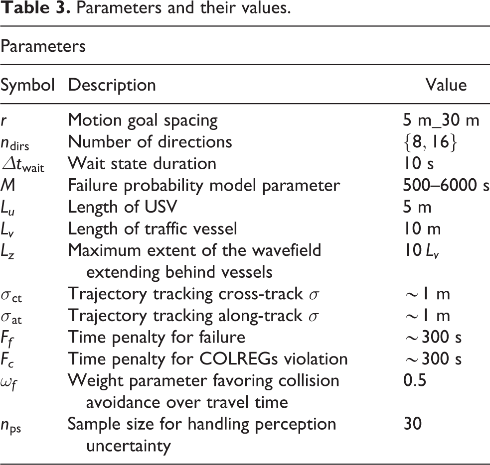
User preference parameters

User preference parameters balance safety and performance. The failure penalty F_f can be chosen as the duration of time required to dispatch a functional USV in lieu of the failed USV. This choice roughly captures the real time impact a failed USV will cause. The COLREGs violation penalty F_c should be much smaller than F_f to favor COLREGs noncompliant trajectories over trajectories that lead to a collision or failure. The extent to which large time delays are accepted to minimize failure is controlled by ω_f. The closer to ω_f is to 1, the more conservative the trajectories are in terms of avoiding failure.

Planning speed parameters

$r, n_{dirs}$ : Decreasing r and increasing n_dirs creates a denser motion goal lattice and thus increases planning times. $Δ t_{wait}$ : Using longer wait state durations, $Δ t_{wait}$ may introduce undesirable looping behavior as the cost of gyrating about a point may be cheaper than waiting at the same point for a duration of $Δ t_{wait}$ . Introducing an extra cost term in equation (8) capturing energy cost will remove this behavior (e.g. $c_{p} = PathLength (n_{p}, n_{c})$ ).

Results

We implemented the wave-aware trajectory planner (WA-TP) in MATLAB on a PC with Intel Xeon 3.5 GHz CPU and 32 GB RAM. A set of simulation experiments were conducted. We discuss the experiments and their results below.

Simulation experiments

We generated four different maps to test the trajectory planner. Traffic vessels at t=0 are shown in Figure 10. The USV and traffic vessels were simulated using three degrees-of-freedom dynamic model as in Klinger et al.⁴⁷ In the USV pose observations used for planning, noise was added following the distribution in equation (6). The response of traffic vessels to the motion of the USV is not simulated. Only the USV is allowed to react to the traffic vessels. Some of the important parameters used are map size = 600 m × 600 m, USV length = $L_{u} = 5 m$ , traffic vessel length = $L_{v} = 10 m$ , traffic vessel speed = $1 - 2 m / s$ . The turning radius and maximum speed of the USV are 5 m and 2 m/s, respectively. The other parameters are presented in Table 3. The traffic vessels are positioned to result in interesting dynamic obstacle avoidance, as well as wavefield crossing behavior. We compare our approach (WA-TP) with three different configurations of the planning stack. These configurations are summarized in Table 4. Global path planner (G-PP) does not consider the dynamic obstacles and generates only kinematically feasible paths to the goal. It is realized by removing dynamic obstacles and removing the time dimension from the implementation of WA-TP. Conservative trajectory planner (C-TP) takes into consideration the traffic vessels along with their wavefields as a nonpermeable dynamic obstacles. This yields conservative trajectories. C-TP is realized by setting M=0 within the wavefield in the implementation of WA-TP. The configuration G-PP + C-VO follows the generated path and avoids traffic vessels using conservative velocity obstacles (C-VOs). C-VO considers traffic vessels along with their wavefields as large obstacles. Velocity obstacle (VO) was not designed to handle waves. Therefore, combining G-PP with VO will lead to the vehicle going over the waves and a high rate of failures. Therefore, we only evaluated G-PP + C-VO combination instead of G-PP + VO.

Figure 10.

Illustration of test maps. Magenta arrows on traffic vessels indicate the direction of motion. Sampling regions for start and goal poses are also shown. An example of a planned trajectory is shown as a red curve. The colored dots in front of the USV represent the set of velocity vectors that considered by the velocity obstacle avoidance method.

Table 4.

Planning stack configurations.

Is feature enabled?
Traffic vessel sensing	Wavefield	VO	Resulting configuration
✗	✗	✓	G-PP + C-VO
✓	✓ (M=0)	✓	C-TP + VO
✓	✓	✓	WA-TP + VO

G-PP: global path planner; C-VO: conservative velocity obstacle; VO: velocity obstacle; WA-TP: wave-aware trajectory planner; C-TP: conservative trajectory planner.

The configuration C-TP + VO follows the conservative trajectory generated by C-TP and avoids traffic vessels using regular VO.

We tested random start and goal poses sampled from the sampling regions, as shown in Figure 10. For each sampled pair, we collected aggregated performance metrics for 20 runs of different configurations of the planning stack. Table 5 presents the execution time, collision count, and success probability. For each run, normalized execution time is computed relative to the execution time of WA-TP. Success probability is computed after each run by using the executed trajectory as in Cost assessment. The results show that WA-TP+VO generally reduces execution time with the exception of M1. However, G-PP + C-VO incurs collisions in M1 as planning without the time dimension results in situations where collision is inevitable. This is also the case in M3 as well. Going into the busy channel just because it is a shorter route to the goal is dangerous and time-consuming. Furthermore, the success probabilities are greatly reduced in G-PP + C-VO as the USV traverses wavefields without proper alignment. On the other hand, C-TP + VO plans longer routes to prevent collisions and ensure higher success probability. This results in increased execution time compared to WA-TP + VO. This is especially evident in M3 where the USV has to cross a busy channel to reach the goal point. C-TP + VO waits for a completely clear channel, whereas WA-TP + VO waits for an opportune moment where the wavefields are traversable.

Table 5.

Comparison of performance.

Metric (avg.)	Map	G-PP + C-VO	C-TP + VO	WA-TP + VO
Normalized execution time	M1	0.87	1.34	1.0
	M2	1.26	1.60	1.0
	M3	1.74	2.04	1.0
Collision count	M1	2	0	0
	M2	3	0	0
	M3	17	0	0
Success probability	M1	0.18	1.0	1.0
	M2	0.32	0.99	0.97
	M3	0.0	0.99	0.98

G-PP: global path planner; C-VO: conservative velocity obstacle; VO: velocity obstacle; WA-TP: wave-aware trajectory planner; C-TP: conservative trajectory planner.

Sensitivity to speed-up techniques

The planner was invoked in the test maps (M1, M2, M3) enabling and disabling subsets of these techniques to study the effects of speed-up techniques. Twenty start and goal points were randomly sampled in the sampling regions corresponding to each map. The baseline configuration of the planner uses Euclidean distance-based time heuristic (i.e. $h (s, g)$ = time taken using straight-line path from s to g using maximum speed). Also, the finest motion goal set and a sample size of $n_{ps} = 30$ is used. The results are presented in Table 6. SOH greatly reduces expansion count and planning time. Among the two heuristics (SOH and space–time exploration heuristics (STEH)), the effect of SOH and STEH is roughly equivalent in maps that do not have heavy dynamic obstacle traffic (M1, M2). In fact, there is an overhead of computing STEH, and it may increase planning time. However, in M3, where the dynamic obstacle traffic is heavy, STEH provides better heuristics compared to SOH due to the added time dimension. In M3, SOH guides the search through the busy channel, whereas STEH guides the search to go around the congestion and head south toward the central channel. In environments with heavy dynamic obstacle traffic, the overhead of computing STEH is justified. Using adaptive motion goals reduces the expansion count further and increases the solution cost at worst by 9%.

Table 6.

Impact of speed-up techniques on performance.

Speed-up technique	Expansion count			Planning time			Solution cost
Speed-up technique	M1	M2	M3	M1	M2	M3	M1	M2	M3
Baseline	1	1	1	1	1	1	1	1	1
SOH	0.257	0.702	0.224	0.224	0.855	0.229	1.016	1.000	1.003
STEH	0.219	0.403	0.132	0.285	0.621	0.162	1.034	1.048	1.032
STEH + AMGS	0.191	0.161	0.103	0.275	0.403	0.116	1.041	1.088	1.054

SOH: static obstacle heuristics; STEH: space–time exploration heuristics; AMGS: adaptive motion goal set.

Sensitivity to MTBF parameter

We illustrate the effects of changing the MTBF parameter of the failure model summarized in Table 2. Figure 11 shows the initial configuration of USV and traffic vessels in the islands map. Traffic vessels were initialized to speeds between 1 m/s and 2 m/s. The USV was set up to use WA-TP + VO and commanded to cross the busy channel (Figure 11). In this experiment, the parameter controlling the danger level of the wave region (i.e. MTBF value M_t ) is changed. Two different values of M_t are used to simulate two different levels of danger. In Figure 12(a), the wavefields are made to be dangerous by assigning a lower MTBF parameter ( $M_{t} = 1000$ ). This results in the USV take a longer trajectory to reach the goal point while altogether avoiding any contact with the wavefield. In Figure 12(b), the wavefields are made to be permeable by assigning a high MTBF parameter ( $M_{t} = 3000$ ), making the traversal of the wavefield less dangerous. Thus, in this case, the USV attempts crossing the wavefield at an appropriate angle as it makes it way to the goal point.

Figure 11.

Scenario to illustrate the effects of changing the MTBF parameter M_t . USV is positioned at the start point and commanded to reach the goal point. The colored dots in front of the USV represent the set of velocity vectors that considered by the velocity-obstacle avoidance method. MTBF: mean-time-between-failures.

Figure 12.

(a) Case $M_{t} = 1000$ . At $t = 75.0$ , the USV avoids crossing the wavefield and takes a longer route to the goal point. Finally, it reaches the goal point at $t = 166.1$ . (b) Case $M_{t} = 3000$ . At $t = 62.0$ , the USV crosses the wavefield at the appropriate angle and reaches the goal point at $t = 139.1$ .

Sensitivity to number of dynamic obstacles and perception uncertainty

We also studied how the algorithm scaled when the number of dynamic obstacles was varied. We used the map M4 and varied the number of dynamic obstacles. Random start and goal poses were sampled from the sampling regions. We used this random sampling scheme to ensure the USV interacts with the dynamic obstacles. Figure 13 shows the mean planning time increasing roughly linearly in the number of dynamic obstacles. We used the scenario in Figure 14 to study how our method performs under different levels of perception uncertainty. Figure 15 illustrates the different behaviors exhibited by our method. In Figure 15(a), the USV stops at the mouth of the channel waiting for the traffic vessel to clear the channel. This behavior is due to the high perception uncertainty associated with the sensing of the traffic vessel. Entering the channel in this situation is a risky move. If the channel is entered without an accurate state estimate of the traffic vessel, a collision might be inevitable when the USV is unable to maneuver around the traffic vessel. This behavior is avoided. In Figure 15(b), the USV enters the channel and keeps to the right lane while the traffic vessel is underway. This behavior is due to the low perception uncertainty associated with the sensing of the traffic vessel. The USV avoids the traffic vessel and also complies with COLREGs.

Figure 13.

Sensitivity to number of dynamic obstacles.

Figure 14.

Scenario to illustrate the effects of perception uncertainty.

Figure 15.

(a) Case: High perception uncertainty. For $75 \leq t \leq 153.1$ , the USV waits at the entrance of the channel until the traffic vessel passes through the channel, (b) case: Low perception uncertainty. The USV enters the channel and takes the right lane as the traffic vessel is passing through the channel.

Physical experiments

Experimental setup

A set of physical experiments using a 16 feet WAM-V USV at North Lake, Hollywood, Florida (see Figure 16), was performed to verify the effectiveness of the proposed approach. In place of real static and dynamic obstacles, we introduced virtual obstacles. They were given to the navigation system in lieu of the perception subsystem. This was done to perform the experiments without risking the loss of the WAM-V platform.

Figure 16.

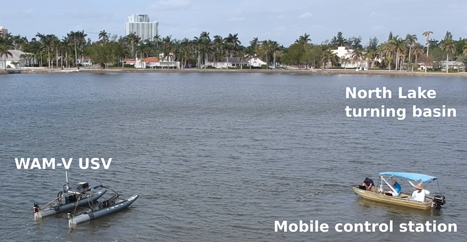
Physical experiment setup.

Figures 17 and 18 show the scenario and the trajectory obtained by WA-TP and C-TP. In these scenarios, dynamic obstacles were moving at constant speeds between 1.0 m/s and 2.0 m/s. During experiments, there was gentle south-easterly winds ranging between 10 and 12 KTS. From Table 7, the execution times are observed to have reduced by as much as 25.1% under the proposed approach. A video clip showing some simulation and physical experiments is located at https://youtu.be/_VGxb4nRUwU.

Figure 17.

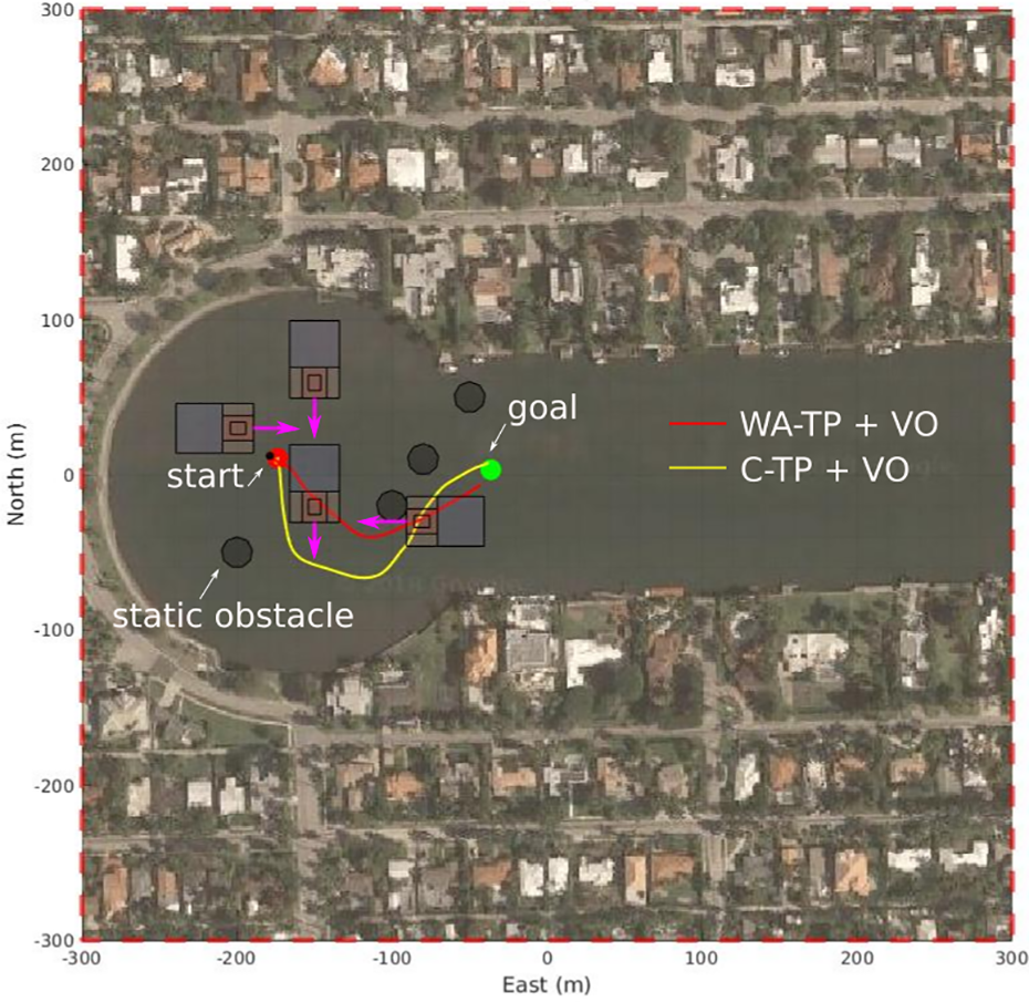
A set of trajectories obtained in scenario P1 comparing wave-aware trajectory with a conservative trajectory.

Figure 18.

A set of trajectories obtained in scenario P₂ comparing wave-aware trajectory with a conservative trajectory.

Table 7.

Comparison of execution time.

Scenario	Planner type	Execution time(s)	Reduction (%)
P1	C-TP + VO	148.9	—
	WA-TP + VO	136.5	8.3
P2	C-TP + VO	163.6	—
	WA-TP + VO	122.5	25.1

Conclusion

Our approach plans trajectories over long distances while avoiding static obstacles and traffic vessels. It also avoids waves generated by them. Our approach executes these trajectories faster and safer. The execution times are reduced by at least 25% when compared to other methods. The proposed approach is able to react safely to varying levels of perception uncertainty. The incorporation of wavefields into the planning process improves the success probability of the planned trajectory. By using heuristics and adaptive motion goal sets, the planning effort and time has been reduced. However, further reduction is required for practical deployment in congested harbors. Harbors have speed limits ranging between 1.8 m/s and 5 m/s and reacting to traffic vessels potentially moving at those speeds requires faster planning times than possible by the current MATLAB implementation. In this work, simplifying assumptions such as trajectory of traffic vessels, the shape and size of the wave regions were made. However, these aspects of the planner can be changed and tuned for specific applications that are not necessarily in the marine domain. The heuristics and evaluation of transition cost under motion/perception uncertainty remain applicable in other domains where there are large semipermeable dynamic obstacles. There are a few potential directions of future work. The reactive behavior of traffic vessels to the actions of the USV was not captured in the planner. Furthermore, wind and current effects were not included in the planning process. These effects can be included when good estimates of the currents and wind direction are available. This will require development of new heuristics. Based on the assumption that multiple traffic vessels may not come very close to the USV, the interaction of wavefields by multiple traffic vessels was ignored. Including this interaction in the planning problem is essential in very congested environments. An optimized C++ implementation can be done for a faster planning time by utilizing GPU and multicore frameworks to perform the computations in the Monte Carlo scheme used for failure probability computations.

Footnotes

Authors’ note

Opinions expressed are those of the authors and do not necessarily reflect the opinions of the sponsors.

Declaration of conflicting interests

The author(s) declared no potential conflicts of interest with respect to the research, authorship, and/or publication of this article.

Funding

The author(s) disclosed receipt of the following financial support for the research, authorship, and/or publication of this article: This work was supported by National Science Foundation (Grant No. #1634433 and #1526016).

ORCID iD

Pradeep Rajendran

S. K. Gupta

Appendix A

References

Wilkie

van den Berg

Manocha

. Generalized velocity obstacles. In: Intelligent Robots and Systems, 2009. IROS 2009. IEEE/RSJ International Conference on, St. Louis, MO, USA, 10–15 October 2009, pp. 5573–5578. IEEE. DOI: 10.1109/IROS.2009.5354175.

Spenko

Kuroda

Dubowsky

, et al. Hazard avoidance for high-speed mobile robots in rough terrain. J Field Robot 2006; 23(5): 311–331.

Berglund

Brodnik

Jonsson

, et al. Planning smooth and obstacle-avoiding b-spline paths for autonomous mining vehicles. IEEE Trans Auto Sci Eng 2010; 7(1): 167–172.

Rajendran

Shah

Gupta

. Dynamics-aware reactive planning for unmanned ground vehicles to avoid collisions with dynamic obstacles on uneven terrains. In: Workshop on Planning and Robotics (PlanRob), held at International Conference on Automated Planning and Scheduling (ICAPS’ 17), Pittsburgh, PA, 19–20 June 2017, pp. 80–91.

Paulos

Eckenstein

Tosun

, et al. Automated self-assembly of large maritime structures by a team of robotic boats. IEEE Trans Auto Sci Eng 2015; 12(3): 958–968.

Likhachev

Ferguson

. Planning long dynamically feasible maneuvers for autonomous vehicles. Int J Rob Res 2009; 28(8): 933–945.

Chi

Wang

, et al. Risk-DTRRT-based optimal motion planning algorithm for mobile robots. IEEE Trans Auto Sci Eng 2018; 16(3): 1–18.

Fulgenzi

Tay

Spalanzani

, et al. Probabilistic navigation in dynamic environment using rapidly-exploring random trees and gaussian processes. In: 2008 IEEE/RSJ International Conference on Intelligent Robots and Systems, Acropolis Convention Center, Nice, France, September 22–26, 2008, pp. 1056–1062. IEEE. DOI:10.1109/IROS.2008.4650959.

Kelly

Nagy

. Reactive nonholonomic trajectory generation via parametric optimal control. Int J Robot Res 2003; 22(7-8): 583–601.

10.

Wei

Dolan

, et al. A real-time motion planner with trajectory optimization for autonomous vehicles. In: 2012 IEEE International Conference on Robotics and Automation, St Paul, MN, May 14–19, 2012, pp. 2061–2067. DOI:10.1109/ICRA.2012.6225063.

11.

Svec

Schwartz

Thakur

, et al. Trajectory planning with look-ahead for unmanned sea surface vehicles to handle environmental disturbances. In: 2011 IEEE/RSJ International Conference on Intelligent Robots and Systems, San Francisco, CA, 25–30 September 2011, pp. 1154–1159. DOI:10.1109/IROS.2011.6095021.

12.

Thakur

Svec

Gupta

. GPU based generation of state transition models using simulations for unmanned surface vehicle trajectory planning. Robot Auto Sys 2012; 60(12): 1457–1471.

13.

Liu

Sukhatme

. A solution to time-varying Markov decision processes 2018. Available at: https://arxiv.org/pdf/1605.01018.pdf.

14.

Kaelbling

Littman

Cassandra

. Planning and acting in partially observable stochastic domains. Artif Intell 1998; 101(1): 99–134.

15.

Roy

Thrun

. Coastal navigation with mobile robots. In: Proceedings of Advances in Neural Information Processing Systems (NIPS ’99), January 1999, pp. 1043–1049. Cambridge: MIT Press.

16.

Silver

Veness

. Monte-Carlo planning in large POMDPs. In: Advances in Neural Information Processing Systems 2010, pp. 2164–2172.

17.

Somani

Hsu

, et al. DESPOT: Online POMDP Planning with Regularization. In: Advances in Neural Information Processing Systems 26 (eds. Burges

CJC

Bottou

Welling

, et al.), 2013, pp. 1772–1780. Curran Associates, Inc. http://papers.nips.cc/paper/5189-despot-online-pomdp-planning-with-regularization.pdf

18.

Rajendran

Moscicki

Wampler

, et al. Wave-aware trajectory planning for unmanned surface vehicles operating in congested environments. In: IEEE International Symposium on Safety, Security and Rescue Robotics (SSRR), 2018.

19.

Chen

Rickert

Knoll

. Motion planning under perception and control uncertainties with space exploration guided heuristic search. In: IEEE Intelligent Vehicles Symposium, Proceedings, 2017, pp. 712–718.

20.

Agha-mohammadi

Chakravorty

Amato

. Firm: feedback controller-based information-state roadmap—a framework for motion planning under uncertainty. In: 2011 IEEE/RSJ International Conference on Intelligent Robots and Systems, San Francisco, California, 25–30 September 2011, pp. 4284–4291. DOI:10.1109/IROS.2011.6095010.

21.

Blackmore

Ono

Williams

. Chance-constrained optimal path planning with obstacles. IEEE Trans Robot 2011; 27(6): 1080–1094.

22.

Censi

Calisi

Luca

, et al. A Bayesian framework for optimal motion planning with uncertainty. In: 2008 IEEE International Conference on Robotics and Automation, Pasadena, CA, 19–23 May 2008, pp. 1798–1805. DOI:10.1109/ROBOT.2008.4543469.

23.

Lenz

Rickert

Knoll

Heuristic search in belief space for motion planning under uncertainties. In: 2015 IEEE/RSJ International Conference on Intelligent Robots and Systems (IROS), Hamburg, Germany, September 28 to October 03, 2015, pp. 2659–2665. DOI:10.1109/IROS.2015.7353740.

24.

Mellinger

Kumar

. Control and planning for vehicles with uncertainty in dynamics. In: 2010 IEEE International Conference on Robotics and Automation, Anchorage, Alaska, May 3–8, 2010, pp. 960–965. DOI:10.1109/ROBOT.2010.5509794.

25.

Stancliff

Dolan

Trebi-Ollennu

Towards a predictive model of mobile robot reliability. Technical Report CMU-RI-TR-05-38, Pittsburgh, PA, 2005.

26.

Greytak

Hover

. Motion planning with an analytic risk cost for holonomic vehicles. In: Proceedings of the 48h IEEE Conference on Decision and Control (CDC) held jointly with 2009 28th Chinese Control Conference, Shanghai, China, 15–18 December 2009, pp. 5655–5660. IEEE. DOI:10.1109/CDC.2009.5399943.

27.

Zhang

Rachmawati

, et al. Exploiting ais data for intelligent maritime navigation: a comprehensive survey from data to methodology. IEEE Trans Intell Transpor Sys 2017; PP(99): 1–24.

28.

Last

Bahlke

Hering-Bertram

, et al. Comprehensive analysis of automatic identification system (AIS) data in regard to vessel movement prediction. J Navig 2014; 67(5): 791–809.

29.

Kim

Lee

Essa

. Gaussian process regression flow for analysis of motion trajectories. In: Proceedings of the 2011 International Conference on Computer Vision, 2011, pp. 1164–1171. USA: IEEE Computer Society. https://doi.org/10.1109/ICCV.2011.6126365

30.

Tiger

Heintz

. Online sparse gaussian process regression for trajectory modeling. In: 2015 18th International Conference on Information Fusion (Fusion), pp. 782–791.

31.

Aoude

Luders

Joseph

, et al. Probabilistically safe motion planning to avoid dynamic obstacles with uncertain motion patterns. Auto Robot 2013; 35(1): 51–76.

32.

Lefèvre

. A survey on motion prediction and risk assessment for intelligent vehicles. Robomech J 2014; 1(1): 1–14.

33.

Hilmer

Thornhill

. Observations of predictive skill for real-time deterministic sea waves from the WaMoS II. In: OCEANS 2015—MTS/IEEE Washington, pp. 1–7. DOI:10.23919/OCEANS.2015.7404496.

34.

Kusters

Cockrell

Connell

BSH

, et al. Futurewaves: a real-time ship motion forecasting system employing advanced wave-sensing radar. In: OCEANS 2016 MTS/IEEE Monterey, pp. 1–9. DOI:10.1109/OCEANS.2016.7761478.

35.

Delsart

Fraichard

Tiji, a generic trajectory generation tool for motion planning and control. In: 2010 IEEE/RSJ International Conference on Intelligent Robots and Systems, Taipei, Taiwan, October 18–22, 2010, pp. 1439–1444. DOI:10.1109/IROS.2010.5648826.

36.

Dubins

. On curves of minimal length with a constraint on average curvature, and with prescribed initial and terminal positions and tangents. Am J Math 1957; 79(3): 497–516. Available at: http://www.jstor.org/stable/2372560.

37.

Sarda

Bertaska

, et al. Station-keeping control of an unmanned surface vehicle exposed to current and wind disturbances. Ocean Eng 2016; 127: 305–324.

38.

Fossen

. Guidance and Control of Ocean Vehicles. New York, NY: Wiley, 1995.

39.

Daniel

Nash

Koenig

, et al. Theta*: any-angle path planning on grids. J Artif Intell Res 2010; 39: 533–579.

40.

Bry

Roy

Rapidly-exploring random belief trees for motion planning under uncertainty. In: 2011 IEEE International Conference on Robotics and Automation, Shanghai, China, 9–13 May 2011, pp. 723–730. DOI:10.1109/ICRA.2011.5980508.

41.

Tredup

. Dangerous waves and your boat, 2011. Available at: http://www.oceannavigator.com/Ocean-Voyager-2011/Dangerous-waves-and-your-boat/.

42.

Svec

Shah

Bertaska

, et al. Dynamics-aware target following for an autonomous surface vehicle operating under COLREGs in civilian traffic. In: 2013 IEEE/RSJ International Conference on Intelligent Robots and Systems, Tokyo, Japan, November 3–7, 2013, pp. 3871–3878. DOI:10.1109/IROS.2013.6696910.

43.

Shah

Švec

Bertaska

, et al. Resolution-adaptive risk-aware trajectory planning for surface vehicles operating in congested civilian traffic. Auto Robot 2016; 40(7): 1139–1163.

44.

Lambert

Gruyer

Pierre

. A fast Monte Carlo algorithm for collision probability estimation. In: 2008 10th International Conference on Control, Automation, Robotics and Vision, Hanoi, Vietnam, 2–5 December 2008, pp. 406–411. DOI:10.1109/ICARCV.2008.4795553.

45.

Liu

Song

Bucknall

. A practical path planning and navigation algorithm for an unmanned surface vehicle using the fast marching algorithm. In: OCEANS 2015—Genova, pp. 1–7. DOI:10.1109/OCEANS-Genova.2015.7271338.

46.

Arismendi

Álvarez

Garrido

, et al. Nonholonomic motion planning using the fast marching square method. Int J Adv Robot Sys 2015; 12(5): 56.

47.

Klinger

Bertaska

von Ellenrieder

, et al. Control of an unmanned surface vehicle with uncertain displacement and drag. IEEE J Oceanic Eng 2016; 42(2): 458–476.

Trajectory planning for unmanned surface vehicles operating under wave-induced motion uncertainty in dynamic environments

Abstract

Keywords

Introduction

Related work

Trajectory planning

Trajectory and wave prediction

Preliminaries and problem formulation

Vehicle model

Traffic vessel profiles

Environmental disturbances

Failure model

Problem formulation

Approach

Node expansion and cost functions

Obtaining tracking error and failure model parameters

Determining tracking error parameters

Determining MTBF

Cost assessment

Accounting for perception uncertainty

Speed-up techniques

Static obstacle heuristics

Space–time exploration heuristics

Adaptive motion goal set

Selection of parameters

User preference parameters

Planning speed parameters

Results

Simulation experiments

Sensitivity to speed-up techniques

Sensitivity to MTBF parameter

Sensitivity to number of dynamic obstacles and perception uncertainty

Physical experiments

Experimental setup

Conclusion

Footnotes

Authors’ note

Declaration of conflicting interests

Funding

ORCID iD

Appendix A

References