Sage Journals: Discover world-class research

Abstract

In this article, we propose a road detection method based on the fusion of Lidar and image data under the framework of conditional random field. Firstly, Lidar point clouds are projected into the monocular images by cross calibration to get the sparse height images, and then we get high-resolution height images via a joint bilateral filter. Then, for all the training image pixels which have corresponding Lidar points, we extract their features from color image and Lidar point clouds, respectively, and use these features together with the location features to train an Adaboost classifier. After that, all the testing pixels are classified into road or non-road under a conditional random field framework. In this conditional random field framework, we use the scores computed from the Adaboost classifier as the unary potential and take the height value of each pixel and its color information into consideration together for the pairwise potential. Finally, experimental tests have been carried out on the KITTI Road data set, and the results show that our method performs well on this data set.

Keywords

Road detection conditional random field multi-sensor fusion robotic vision autonomous vehicles

Introduction

Road detection is always a key problem in autonomous driving. For its driving safety, an unmanned ground vehicle must have the ability to distinguish road or free space from obstacles in various environments, as well as to obey the traffic rules. Over the last decades, many different methods have been proposed to deal with this problem. However, due to the complex surroundings and obstacles in different environments, as well as various lighting conditions, road detection is still a challenging task.

Many road detection methods based on monocular images have been proposed. Compared with other sensors, the monocular visible light camera is much cheaper so that it can be widely used for this task. Nowadays, with the rapid development of the 3-D sensors, more and more road detection methods are based on the stereo vision or laser range finder. For example, Kinect, a cheap 3-D sensor that can provide the dense depth map registered with an RGB image (RGB-D) is widely used in the indoor scenes. On the other hand, in the outdoor scenes, the most common kind of 3-D sensors is the light detection and ranging (Lidar), such as the Velodyne HDL-64E (Velodyne LIDAR, USA). This kind of sensors can provide 3-D range data in the form of point clouds, which have maximum ranges of 60–80 m.

The 3-D sensors have many advantages, for example, they can provide the 3-D structure information and they are robust to the changing of lighting conditions. However, they also have some weaknesses. For example, stereo vision sensor is sensitive to the noises and object movements in the environment, and the Lidar can only generate very sparse data of distant objects without color information, which is helpful to detect the road areas. Therefore, fusion of data from different kinds of sensors is a better way for road detection.

However, even though many methods have been proposed, the road detection still remains an open problem, and that is because most of the proposed methods only extract low-level features from image and Lidar data and then fuse them in feature level to train a classifier to detect road. In order to improve the performance of road detection, in this article, we propose a road detection method based on multi-sensors and try to fuse data in both data level and feature level. To be more specific, in our method, firstly, we project the Lidar point clouds into the images and obtain original height images which are sparse. Then, we upsample these height images via a joint bilateral filter so that all pixels will have their own height values. For each image pixel which has its original corresponding Lidar points, we extract the textons features,¹ the Lidar-based features, and the location features. After that, we use conditional random field (CRF) framework to classify each pixel into road pixel or non-road pixel. Under this CRF framework, all the extracted features are used to train an Adaboost classifier, and the scores computed from this classifier are considered as the unary potential. At the same time, the differences in color values and height values of pixels are taken into consideration as the pairwise potential. Then, it is optimized with graph cuts. Experimental tests have been carried out on the KITTI Road data set,² and the results show that our method performs well.

This article is organized as follows: Firstly, the related works are briefly reviewed. Then our method is given in detail. After that, we show our experimental results on KITTI Road benchmark, and finally, we conclude our article.

Related works

A variety of road detection methods have been proposed in the last decades. Among these methods, two different kinds of sensors are used individually or jointly: the monocular vision sensors (visible light cameras) and the 3-D sensors (including stereo vision sensors and the Lidar sensors).

There are lots of road detection methods based on the monocular vision sensors. Since this kind of sensors is very cheap, it has been used in this task for decades. Most of these methods use low-level features of pixels, such as texture, edge, or color, to separate the road areas from non-road areas. For example, Malik et al.¹ designed an N-dimensional filter bank and convolved images with it to get responses of every pixels as their textons features. This kind of feature has been proven to be effective, and some other improved methods based on that were also proposed.^3,4 Besides, these methods often make the assumption that the particular part of the images, such as the lower part of the images, is more likely to be the road part.³ Except for the low-level features, some researches use contextual cues to improve the results. For example, Alvarez and Lopez⁵ proposed a method that combined the context, including horizon lines, vanishing points, lane markings, and so on, with low-level cues to detect road, making the method robust to varying imaging conditions.

Some other methods used the data from 3-D sensors (such as stereo camera or Lidar sensors) or fused data from 3-D sensors and monocular cameras to detect the road area. Nanri et al.⁶ proposed a method to compute height changes against road surface on several multi-directional scanning lines from the dense disparity map, and they can detect a variety of road boundaries even with unsmooth edges or jagged boundaries. Suger et al.⁷ generated a 2-D grid map from 3-D points and extracted features from every individual cells. This kind of features contained five measurements: the absolute maximum difference in the z-coordinate, the mean of the remission values, the variance of the remission values, the roughness, and the slope of the cell. Xiao et al.⁴ fused the Lidar data and monocular image under the framework of CRF to detect the road. In their method, they used the pixel-wise texture, dense histogram of oriented gradients (dense HOG), color and location cues as the image features, and the normalized 3-D location and the direction of the local normal vector of every point as the Lidar features. Shinzato et al.⁸ also proposed a road terrain detection method via sensors fusion, they used spatial relationship in image perspective view combined with real 3-D metric values to determine whether a point corresponds to an obstacle or not. After that, they used polar histograms to generate a confidence map that represented the road areas in the images.

In our method, we also detect road areas based on the fusion of Lidar and image data. However, in those methods mentioned above, they usually extract low-level Lidar–based features, such as the absolute maximum in heights, the mean of heights, the normal vector, and so on, to fuse with image-based features. Compared to them, we propose a Lidar-based feature which can describe the distribution of one Lidar point and its neighbors. Besides, we project Lidar point clouds into the images to generate dense height images and use these height images in our CRF framework to eliminate the effects of shadows on the road surface.

Road detection based on Lidar and image fusion

Height image upsampling

Usually, the different illumination conditions have great impact on the color differences. Therefore, removing shadows from the road surface can greatly improve the performance of road detection.⁵ The most popular way to deal with this problem is to convert the color images into “shadow-free” images, which are not sensitive to the lighting conditions. For example, Alvarez and Lopez⁹ proposed a method that converted images from RGB channels into shadow-invariant feature channel. They used r = log(R/G) and b = log(B/G) to take replace of R, G, and B, which means each pixel P_i = (R_i ,G_i ,B_i ) in RGB images is now converted into P′_i = (r_i ,b_i ). And then they are projected into a line l_θ, where θ was the direction of the line. After that, we denote the distance between projection results of P′_i = (r_i ,b_i ) and P′₀ = (0,0) as each pixel’s value in shadow-free channel. These converted images are named as shadow-free images.

However, as shown in Figure 1, the shadow-free image has many noises, and some road edges, for example, the left curb on the image becomes unclear. Therefore, instead of using those shadow-free images, we generate height images by fusing Lidar and image data and use these height images to eliminate the influence of the shadow while keeping the edges clear as well.

Figure 1.

The shadow-free image and the height image. The first row is the color image, the second row is the shadow-free image, and the third row is the high-resolution height image.

As we mentioned above, some other methods also use height smoothness or height change to detect road areas,⁶ but unlike only using heights of Lidar points, we try to obtain the heights of every image pixels and generate the dense height images. In order to do this, firstly, we fuse the Lidar point clouds and color images by transforming the 3-D points $P_{lidar} = {X, Y, Z}$ in 3-D Lidar coordinate system into 2-D points $P_{camera} = {U, V}$ in camera coordinate system. Based on the calibration, the transformation equation is as follows

P_{camera} = R_{rect}^{0} T_{lidar}^{camera} P_{lidar}

where $R_{rect}^{0}$ is the rotation matrix from raw-image-camera to rectified-image-camera and $T_{lidar}^{camera}$ is the transformation matrix. To be more specific, $T_{lidar}^{camera}$ is as follows

T_{lidar}^{camera} = [\begin{matrix} R_{lidar}^{camera} & t_{lidar}^{camera} \\ 0 & 1 \end{matrix}]

where $R_{lidar}^{camera}$ is the rotation matrix and $t_{lidar}^{camera}$ is the translation matrix. They are used to transform a point from Lidar coordinate into the camera coordinate.

Usually, such matrixes are pre-calculated on some data set such as KITTI. Therefore, in our method, we assume that those matrixes are calculated in advance. For more details, refer to Geiger’s works.^10,11

After the projection, some of the image pixels have their heights while the others not. These sparse height images have to be upsampled to generate high-resolution smooth and dense height images. Generally, there are two kinds of methods to upsample these images, one of them is based on MRF frameworks^12,13 and the other is based on joint bilateral filters.^14
–16 In our method, we choose the joint bilateral filter to upsample height images. The joint bilateral filter is based on the assumption that areas of similar color usually have similar height values. Just like the methods we mentioned above,^14
–16 the joint bilateral filter we use can be formalized as

{\hat{H}}_{i} = \frac{1}{α} \sum_{j \in N_{i}} W_{(i, j)}^{1} W_{(i, j)}^{2} H_{j}

W_{(i, j)}^{1} = {exp}^{- | | C_{i} - C_{j} {| |}^{2} / 2 σ_{1}^{2}}

W_{(i, j)}^{2} = {exp}^{- | | i - j {| |}^{2} / 2 σ_{2}^{2}}

where α is a normalizing factor, which ensures weights sum to one, ${\hat{H}}_{i}$ is the new height value of the pixel $p_{i} = (u_{i}, v_{i})$ , N_i is the neighborhood of P_i, $W_{(i, j)}^{1}$ and $W_{(i, j)}^{2}$ are Gaussian with standard deviation weights, $| | C_{i} - C_{j} | |$ is the Euclidean distance between P_i and P_j in color channels, and $| | i - j | |$ is the Euclidean distance between pixel position i and position j. In a word, each height value is replaced by a weighted combination of its neighboring height values.

As shown in Figure 2, after the upsampling processing, all the pixels have their height values.

Figure 2.

The upsampling of height image. The first row is the color image, the second row is the low-resolution height image, and the third row is the high-resolution height image.

Feature extraction

The unary potential of the CRF we use is the negative log likelihood of variable X_i taking label x_i: $ψ_{i} (x_{i}) = - log p (x_{i})$ , where p(x_i) is the probability of being road of X_i, which is generated by a learned Adaboost classifier. To train such classifier, we extract the following features: the textons features based on color images, the Lidar-based features, and the location features.

Textons features are the responses of Filter Bank³ on color images. The Filter Bank consists of Gaussians at scales k, 2k, and 4k; x and y derivatives of Gaussians at scales 2k and 4k; and Laplacians of Gaussians at scales k, 2k, 4k, and 8k. After we convert the images into the Lab color space, the Gaussian filters are applied to all three color channels, while the other filters are applied only to the L channel. Finally, we can get an 18-dimension vector for each pixel.

We also propose a Lidar-based feature named local distance distribution (LDD). To be specific, a neighborhood η for a 3-D point $p_{i} = {x_{i}, y_{i}, z_{i}}$ is defined, in which the Euclidean distance D_ij between P_i and $P_{j} (j \in η)$ is less than a threshold γ_D. In practice, γ_D is usually between 0.3 m and 0.5 m. Then, all the neighborhood space is equally divided into M * N * K spatial cells. For a point P_i, the distribution histogram $H_{s}, s = {1, 2, ..., M * N * K}$ in Cell_s is defined as follows

H_{s} = \frac{\sum_{k \in {Cell}_{s}} D_{i k}}{\sum_{j \in η} D_{i j}}

Therefore, the LDD feature of point P_i is an N*M*K-dimensional feature $H = {H_{1}, H_{2},..., H_{M * N * K}}$ . Figure 3 shows how to extract LDD features.

Figure 3.

The extraction of LDD features. LDD: local distance distribution.

Besides, since the middle lower parts of the images are more likely to be road, we also use the locations of the pixels in the images as the location features.

CRF for road detection

Since Shotton et al.¹⁷ firstly used CRF in semantic labeling, there have been many variants proposed after that. Road detection can be seen as a two-class (road and non-road) labeling problem, in which each pixel p_i is modeled as a discrete random variable $x_{i} \in L$ with $L = {road, non-road}$ being its label and $i \in V = {1, 2, ..., N}$ . A clique C is a set of random variables x_c which are conditionally dependent on each other.

For a given observed image I, the posterior probability of the labeling is a Gibbs distribution and can be written as

P (x | Y) = \frac{1}{Z} exp (\sum_{c \in C} - ψ_{c} (x_{c}))

where $Z = \sum_{x} exp (\sum_{c \in C} - ψ_{c} (x_{c}))$ is a normalizing constant, C is the set of all cliques, and ψ_c is the potential function of clique c. Therefore, the corresponding Gibbs energy is as follows

E (x) = - log P (x | Y) - log Z = \sum_{c \in C} ψ_{c} (x_{c})

Then, the most possible labeling result of X can be written as

x^{*} = \underset{x \in L}{argmax} P (x | Y) = \underset{x \in L}{argmin} E (x)

For most of the methods, the pixel labeling problems can be formulated as pairwise CRFs, which only consider the unary potential and pairwise potential. And usually the neighborhood relationship in these CRFs is defined as locally four-connected or eight-connected neighborhood. Their energies can be written as the sum of unary and pairwise potentials

E (x) = \sum_{i \in V} ψ_{i} (x_{i}) + \sum_{i \in V, j \in N_{i}} ψ_{i j} (x_{i}, x_{j})

where the unary potential $ψ_{i} (x_{i})$ of the CRF is defined as the negative log likelihood of variable X_i taking label x_i: $ψ_{i} (x_{i}) = - log p (x_{i})$ . In our method, for those pixels which have their corresponding Lidar points, the p(x_i) are the scores computed by the learned Adaboost classifier, while for other pixels, p(x_i) are set as 0.5.

The pairwise potential encodes a smoothness prior which encourages neighboring pixels in the image to have the same labels. Usually, the pairwise potential $ψ_{i j} (x_{i}, x_{j})$ is only related to the color difference between P_i and P_j, but since we have generated the height images to resist the influences of shadows, we can now rewrite the pairwise potential as follows

ω_{1} = exp (- \frac{| | I_{i} - I_{j} {| |}_{2}^{2}}{2 β_{1}})

ω_{2} = exp (- \frac{| | H_{i} - H_{j} | |}{2 β_{2}})

ψ_{i j} (x_{i}, x_{j}) = {\begin{array}{l} 0, & if x_{i} = x_{j} \\ γ \frac{1}{D_{i j}} (λ_{1} ω_{1} + λ_{2} ω_{2}), & otherwise \end{array}

where γ is the trade-off parameter between the unary potential and the pairwise potential, λ₁ and λ₂ are parameters to balance the weights of height difference and color difference, D_ij is the Euclidean distance between the pixel points P_i and P_j, I_i and H_i are the color value (in RGB channels) and the height value of pixel point P_i, respectively, and β₁ and β₂ are two deviations.

There are many ways to solve the energy minimization problem under CRF framework. In our work, we use α-expansion method which is available from an open source library named graph cuts optimization (GCO).^18
–20 For more details, refer to their work.

Experiments

Data sets

In order to test the performance of our proposed method, we use the KITTI Road data set as benchmark. This data set contains 579 frames of color images, Lidar point clouds, and their calibration parameters. The average spatial resolution of the images is 1242 × 375 px. For this data set, 289 frames are as the training data and 290 frames are as the testing data.

All the data are divided into three different categories and each category belongs to one road scenes: urban marked (UM), urban multiple marked (UMM) lanes, and urban unmarked (UU). Figure 4 shows some of the scenes of these three categories. From Figure 4, we can see that the environment surroundings and the lighting conditions are quite variable.

Figure 4.

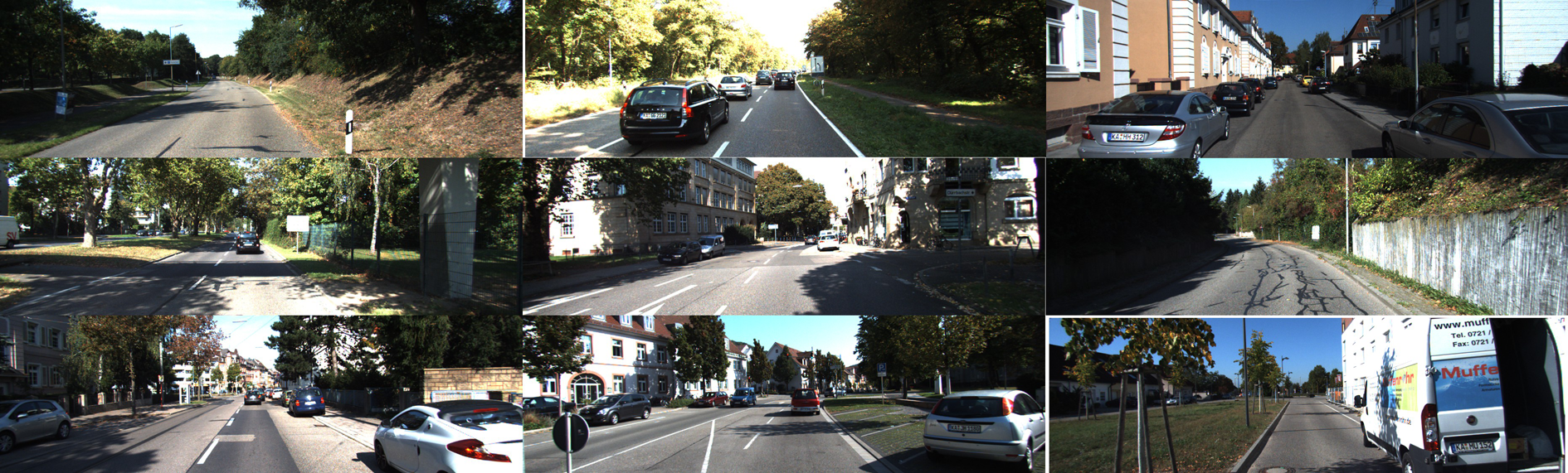
Some scenes of different road categories. Three images in the left column belong to UM, three images in the middle column belong to UMM, and three images in the right column belong to UU. UM: urban marked; UMM: urban multiple marked; UU: urban unmarked.

Our method only detects the road areas and does not consider the lane information. For evaluation, a set of metrics including precision, recall, maximum F1-measure, average precision, false positive rate, and false negative rate are used.

Experimental settings

In the unary potential of our CRF framework, we use the results from Adaboost classifier. And for this classifier, we set decision tree with depth d = 5 as the weak classifier and run for 50 rounds. The parameters of our CRF are analyzed in the following subsections. All the experiments were carried on a PC with 4 GB of RAM and a dual-core Intel Core i5-3230M CPU clocked at 2.6 GHz, and the code is written in C++ and Matlab environment. The average time of processing a frame of testing data is 6.3 s.

Lidar-based features

In this subsection, we will present the road detection performances of different kinds of Lidar-based features. The Lidar data are in the form of point clouds: $P_{i} = {x_{i}, y_{i}, z_{i}}$ . Table 1 shows all the kinds of features we test. Since the KITTI data set does not provide the ground truth of the testing data set, we only use the UM training data set, which contains 95 frames to evaluate those methods. The UM training data set is randomly divided into two parts (one contains 47 frames and the other contains 48 frames). Every kinds of Lidar-based features are fused with the textons features to train the classifiers. Besides, while extracting textons features, we only consider those pixels which have their corresponding 3-D points in point clouds. On average, for one frame we only use about 18,000 points. The distance threshold for neighbors D_ij is set to be 0.3 m. Figure 5 shows the experimental results. From this figure, we can see that each kind of Lidar-based features can improve the results compared with the textons features only, and among all the features we test, the LDD performs best.

Table 1.

Different kinds of Lidar-based features.

Features	f_i	Formulation	Description
Point location	f ₁	x	The x of the point location
	f ₂	y	The y of the point location
	f ₃	z	The z of the point location
	f ₄	H _diff	Maximum of height differences among its neighborhood
	f ₅	H _var	Maximum of height variances among its neighborhood
Xiao’s work⁴	f ₁	x	The x of the point location
	f ₂	y	The y of the point location
	f ₃	z	The z of the point location
	f ₄	θ	Direction of the local normal vector
Shinzato’s work⁸	f ₁	x	The x of the point location
	f ₂	y	The y of the point location
	f ₃	z	The z of the point location
	f ₄	$\frac{- (z_{i} - z_{j})}{\| \| P_{i} - P_{j} \| \|}$	$(z_{i} - z_{j})$ is the difference from height values between two points, $\| \| P_{i} - P_{j} \| \|$ is the vector length from vector $(P_{i} - P_{j})$
LDD	f₁– $f_{M * N * K}$	$H_{i}, i = 1, 2, ..., M * N * K$	The local distance distribution

LDD: local distance distribution.

Figure 5.

The receiver operating characteristic (ROC) curves of road detection based on different kinds of Lidar-based features.

Removing the effects of the shadows

As we mentioned above, removing the shadows from the road surface is very important for road detection. To verify the shadow elimination performances of shadow-free images⁹ and our height images, we convert all the color images from UM training data set to those two kinds of images, respectively. The parameter θ of shadow-free method is 42°. The parameter σ₁ is 10 and σ₂ is 3 of the joint bilateral filter. Then, the UM training dataset is randomly divided into two parts for training and testing, respectively, as we do in the experiments above. After that, we train two different CRF frameworks to detect road. In one of which the H_i is the height value of P_i from height images, and in the other, the H_i represents the value in shadow-free channel of P_i from shadow-free images. Table 2 shows the average accuracies of road detection under those two CRFs. From the table, we can see the CRF framework with height images has better performance in detecting the road, and this proves the height images are more effective to eliminate the effects of shadows compared to the shadow-free images.

Table 2.

Average accuracies of road detection under two CRF frameworks.

Kind of images used in CRF	Average accuracy (%)
Shadow-free	86.43
Height	90.33

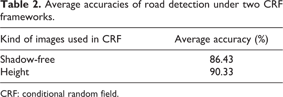
CRF: conditional random field.

Performances

To show the road detection performance of our proposed method, we use all the training data to train an Adaboost classifier and our proposed CRF. All the parameters are set via 10-fold cross validation experiments on the training data set. The parameters M, N, and K of LDD are all 3, and the γ_D of LDD is 0.3 m. Since the GCO can only take integers as the unary potentials, the unary potentials are converted to 0–255. Under such constraint and based on the experiments on the training data set, the parameters of pairwise potential are set empirically as γ is 200, λ₁ is 0.6, λ₂ is 0.4, β₁ is 10, and β₂ is 10. Then, we test our method on the testing data set and evaluate the results in the bird eye view on the KITTI website. Table 3, Figures 6 and 7 show some results.

Table 3.

Results of our method.

Benchmark	MaxF (%)	AP (%)	PRE (%)	REC (%)	FPR (%)	FNR (%)
UM_ROAD	91.57	84.68	90.02	93.19	4.71	6.81
UMM_ROAD	92.75	90.24	94.03	91.50	6.39	8.50
UU_ROAD	85.69	75.12	80.17	92.02	7.42	7.89

MaxF: maximum F1-measure; AP: average precision; PRE: precision; REC: recall, FPR: false positive rate; FNR: false negative rate.

Figure 6.

The evaluations in bird’s eye view. Here, red denotes false negatives, blue areas correspond to false positives, and green represents true positives.

Figure 7.

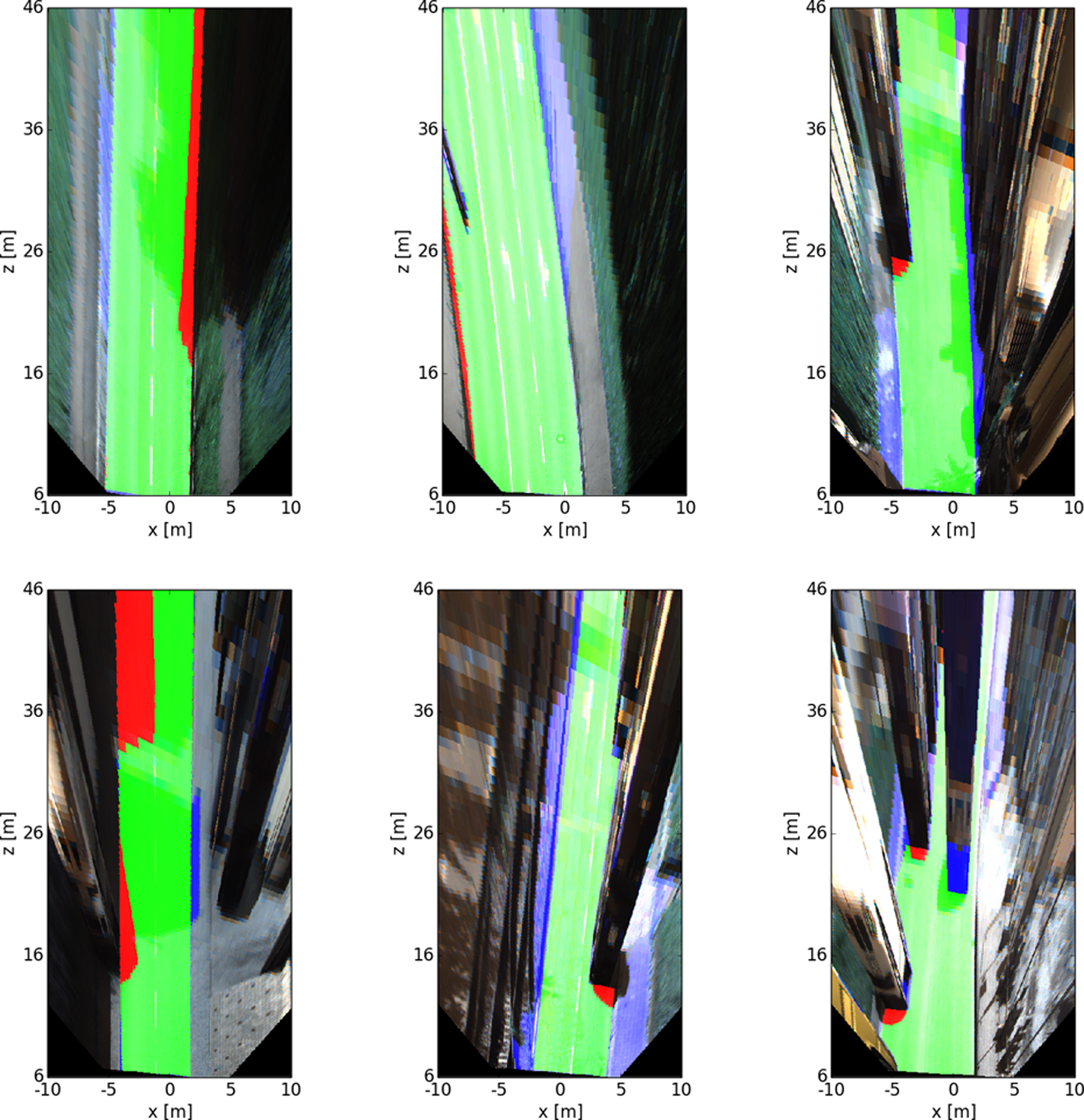
Some results of different road categories. Here, red denotes false negatives, blue areas correspond to false positives, and green represents true positives. The first row belongs to UM, the second rows belong to UMM, and the third row belongs to UU. UM: urban marked; UMM: urban multiple marked; UU: urban unmarked.

We compare our method with some other methods which also used Lidar data or CRF framework, including HybridCRF, FusedCRF,⁴ GRES3D+VELO,⁸ and RES3D-Velo.⁸ The results are shown from Tables 4 to 6. From the tables, we can see that our method performs the best in UM and UMM data set. Although our method performs slightly worse than HybridCRF in UU data set (that may be because we use different image features in the Adaboost classifier), it still outperforms the others overall.

Table 4.

Results of online evaluation on UM (BEV).

Method	MaxF (%)	AP (%)	PRE (%)	REC (%)	FPR (%)	FNR (%)
HybridCRF	90.99	85.26	90.65	91.33	4.29	8.67
FusedCRF	89.55	80.00	84.87	94.78	7.70	5.22
GRES3D+VELO	85.43	83.04	82.69	88.37	8.43	11.63
RES3D-Velo	83.81	73.95	78.56	89.80	11.16	10.20
MixedCRF (our method)	91.57	84.68	90.02	93.19	4.71	6.81

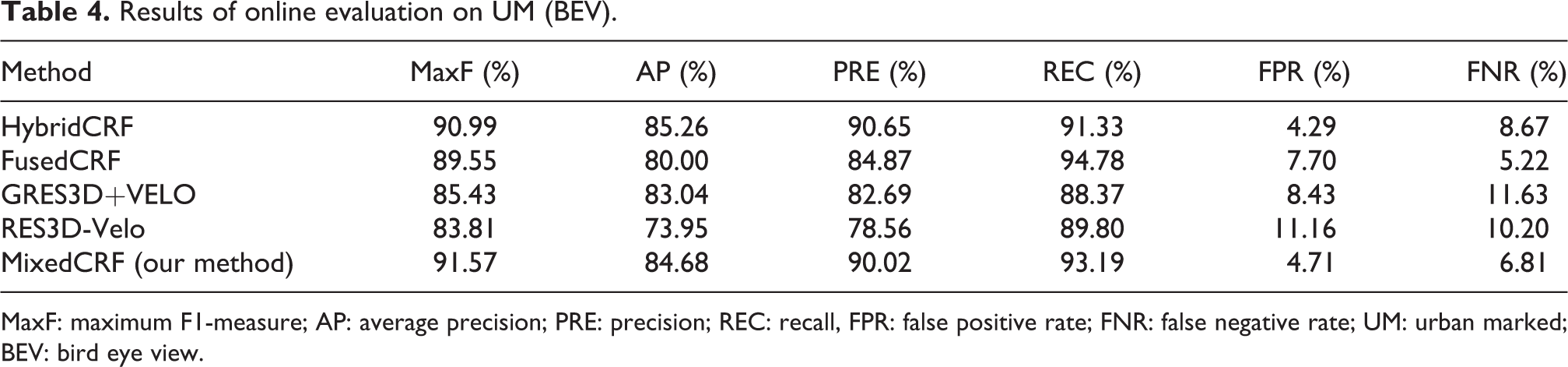
MaxF: maximum F1-measure; AP: average precision; PRE: precision; REC: recall, FPR: false positive rate; FNR: false negative rate; UM: urban marked; BEV: bird eye view.

Table 5.

Results of online evaluation on UMM (BEV).

Method	MaxF (%)	AP (%)	PRE (%)	REC (%)	FPR (%)	FNR (%)
HybridCRF	91.95	86.44	94.01	89.98	6.30	10.02
FusedCRF	89.51	83.53	86.64	92.58	15.69	7.42
GRES3D+VELO	88.19	88.65	83.98	92.85	19.48	7.15
RES3D-Velo	90.60	85.38	85.96	95.78	17.20	4.22
MixedCRF (our method)	92.75	90.24	94.03	91.50	6.39	8.50

MaxF: maximum F1-measure; AP: average precision; PRE: precision; REC: recall, FPR: false positive rate; FNR: false negative rate; UMM: urban multiple marked; BEV: bird eye view.

Table 6.

Results of online evaluation on UU (BEV).

Method	MaxF (%)	AP (%)	PRE (%)	REC (%)	FPR (%)	FNR (%)
HybridCRF	86.79	75.60	86.94	86.64	4.24	13.36
FusedCRF	84.49	72.35	77.13	93.40	9.02	6.60
GRES3D+VELO	84.14	80.20	80.57	88.03	6.92	11.97
RES3D-Velo	83.63	72.58	77.38	90.97	8.67	9.03
MixedCRF (our method)	85.69	75.12	80.17	92.02	7.42	7.89

MaxF: maximum F1-measure; AP: average precision; PRE: precision; REC: recall, FPR: false positive rate; FNR: false negative rate; UU: urban unmarked; BEV: bird eye view.

Discussion

Although we have achieved really good performance on KITTI road benchmark, there are still some limitations of our proposed method. Firstly, there are many false positives of our results, as shown in the first row of Figure 7. This is because the road areas and non-road areas are very similar in colors, textures, and heights, therefore the features extracted from images or Lidar point clouds cannot distinguish them well. Secondly, the second row of Figure 7 shows that, because the Lidar point clouds are sparser and sparser as the distance increases, we have a few false positives in the far areas from the vehicle. These problems should be further studied in our future work.

Conclusion and future works

In this article, we propose a road detection method based on Lidar and image data. Firstly, we project the Lidar points into the images and use a joint bilateral filter to generate the dense height images. Then, we extract the image-based features (textons), Lidar-based features (LDD), and location features to train an Adaboost classifier. After that, we use CRF framework to get the road detection results.

The main contributions of our work are as follows: (1) We propose a Lidar-based feature called LDD, which is effective to describe the spatial relationship of one point and its neighborhood points. This kind of feature is fused with textons features and location features to train an Adaboost classifier, and experimental results show that the fused features can improve the performance of road detection. (2) To resist the influence of shadows on the road surfaces, we use height images together with color images in the pairwise potential of CRF framework. The height images have less noises and more clear edges than traditional shadow-free images, so that we can use them to improve the road detection results under different lighting conditions.

The experiments are carried out on the KITTI Road data set, and the results show that our method performs well. We will try to use our method on more road detection data set to verify its effectiveness in different environments in the future.

Footnotes

Acknowledgements

The authors would like to thank the referees for their comments.

Declaration of conflicting interests

The author(s) declared no potential conflicts of interest with respect to the research, authorship, and/or publication of this article.

Funding

The author(s) disclosed receipt of the following financial support for the research, authorship, and/or publication of this article: This work is supported in part by the National Natural Science Foundation of China (NSFC) (Nos. 61233011, 61403202, and 91220301), by the National Science and Technology Major Project of China (No. 2015ZX01041101), by the 111 Project of China (No. B13022), by the Jiangsu Key Laboratory of Image and Video Understanding for Social Safety (Nanjing University of Science and Technology, China; No. 30920140122007) and by China Post Doctor Foundation (No. 2014M561654).

References

Malik

Belongie

Leung

. Contour and texture analysis for image segmentation. Int J Comput Vis 2001; 43(1): 7–27.

Fritsch

Kuehnl

Geiger

. A new performance measure and evaluation benchmark for road detection algorithms. In: International conference on intelligent transportation systems (ITSC), 2013, pp. 1693–1700.

Shotton

Winn

Rother

. Textonboost for image understanding: multi-class object recognition and segmentation by jointly modeling texture, layout, and context. Int J Comput Vis 2009; 81(1): 2–23.

Xiao

Dai

Liu

. CRF based road detection with multi-sensor fusion. In: Intelligent vehicles symposium, 2015, pp. 192–198.

Alvarez

Lopez

Gevers

. Combining priors, appearance, and context for road detection. IEEE Trans Int Transp Syst 2014; 15(3): 1168–1178.

Nanri

Khiat

Furusho

. General-purpose road boundary detection with stereo camera. In: IAPR international conference on machine vision applications, 2015, pp. 361–364.

Suger

Steder

Burgard

. Traversability analysis for mobile robots in outdoor environments: a semi-supervised learning approach based on 3d-lidar data. In: 2015 Proceedings—IEEE international conference on robotics and automation, 2015, pp. 3941–3946.

Shinzato

Gomes

Wolf

. Road estimation with sparse 3d points from stereo data. In: IEEE international conference on intelligent transportation systems, 2014, pp. 1688–1693.

Alvarez

JMA

Lopez

. Road detection based on illuminant invariance. IEEE Trans Intell Transp Syst 2011; 12(1): 184–193.

10.

Geiger

Lenz

Stiller

. Vision meets robotics: the KITTI dataset. Int J Robot Res 2013; 32(11): 1231–1237.

11.

Geiger

Moosmann

Car

. A toolbox for automatic calibration of range and camera sensors using a single shot. In: Proceedings of International Conference on Robotics and Automation (ICRA), 2012.

12.

Diebel

Thrun

. An application of Markov random fields to range sensing. In: Advances in neural information processing systems, 2006, pp. 291–298.

13.

Liu

Jia

. An MRF-based depth upsampling: upsample the depth map with its own property. IEEE Signal Process Lett 2015; 22(10): 1708–1712.

14.

Kopf

Cohen

Lischinski

. Joint bilateral upsampling. ACM Trans Graph 2007; 26(3): 96.

15.

Yang

Davis

. Spatial-depth super resolution for range images. In: IEEE conference on computer vision & pattern recognition, 2007, pp. 1–8.

16.

Chan

Buisman

Theobalt

. A noise-aware filter for real-time depth upsampling. In: The Workshop on Multi-Camera & Multi-Modal Sensor Fusion Algorithms & Applications, 2008.

17.

Shotton

Winn

Rother

. TextonBoost: joint appearance, shape and context modeling for multi-class object recognition and segmentation. Berlin, Heidelberg: Springer, 2006.

18.

Boykov

Veksler

Zabih

. Fast approximate energy minimization via graph cuts. IEEE Trans Pattern Anal Mach Intell 2001; 23(11): 1222–1239.

19.

Kolmogorov

Zabih

. What energy functions can be minimized via graph cuts? IEEE Trans Pattern Anal Mach Intell 2004; 26(2): 147–159.

20.

Boykov

Kolmogorov

. An experimental comparison of min-cut/max-flow algorithms for energy minimization in vision. IEEE Trans Pattern Anal Mach Intell 2001; 11(26): 1124–1137.

Road detection based on the fusion of Lidar and image data

Abstract

Keywords

Introduction

Related works

Road detection based on Lidar and image fusion

Height image upsampling

Feature extraction

CRF for road detection

Experiments

Data sets

Experimental settings

Lidar-based features

Removing the effects of the shadows

Performances

Discussion

Conclusion and future works

Footnotes

Acknowledgements

Declaration of conflicting interests

Funding

References