Sage Journals: Discover world-class research

Abstract

Free space detection is crucial to autonomous vehicles while existing works are not entirely satisfactory. As cameras have many advantages on environment perception, a stereo vision-based robust free space detection method is proposed which mainly depends on geometry information and Gaussian process regression. In this work, in order to improve the performance by exploiting multiple source information, we apply Bayesian framework and conditional random field inference to fuse the multimodal information including 2-D image and 3-D point geometric information. Particularly, a Bayesian framework is used for multiple feature fusion to provide a normalized and flexible output. Gaussian process regression is used to automatically and incrementally regress the data, resulting enhanced performance. Finally, conditional random field with color and geometry constrains is applied to make the result more robust. In order to evaluate the proposed method, quantitative experiments on popular KITTI-road data set and qualitative experiments on our own campus data set are tested. The results show satisfactory and inspiring performance compared to the outstanding works and even are competitive to some relevant Lidar-based methods.

Keywords

Free space detection Gaussian process regression autonomous vehicle stereo vision multimodal Bayesian fusion

Introduction

Autonomous vehicle has a basic perception task often called “free space detection” which means to seek the ground where is able to traverse from the current location. The mostly used sensor for this task is Lidar which provides accurate 3-D measurement of the environment. However, it is very expensive and cannot capture the content information. On the contrary, camera is very cheap and also can provide dense points with color information. In addition, the great improvement of stereo vision in recent years allows feasible 3-D measurement. Thus, vision-based free space detection becomes very popular.¹

In the previous work,² Lidar-based ground segmentation using Gaussian process regression is very powerful not only in urban but also in rural environment which can be regarded as a versatile algorithm not limited by the scenes as well as pre-trained models. It models the heights of ground points to be jointly Gaussian distributed and applies the Gaussian process regression to incrementally classify the ground points. However, it is not sensitive to the obstacles with low height such as curbstones so that it needs additional curb detection module³ to handle this problem. Actually, the source height as feature is not feasible in many cases because of the bias of calibration and the non-flat ground which both can cause the heights of objects in local coordinate to be inaccurate. Figure 1 shows a simple situation where a wrong height of the obstacle is measured due to the non-flat ground.

Figure 1.

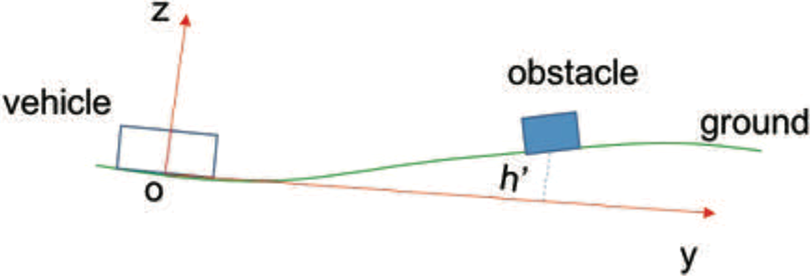
Illustration on the local scene of a vehicle. The non-flat ground makes the obstacle “fly” in the air.

In this article, in order to take advantages of multimodal information, both 2-D image and 3-D space geometric information are used. The method is focused on the 3-D geometry and tries to use a set of simple features to detect free space and applies a flexible fusion framework to improve the previous work without additional modules such as curb detection. The proposed method provides the 3-D points from the stereo for simplicity which is of cause not limited by this way and does not need to make prior assumptions about the geometry of the scenes and is able to detect many types of unstructured obstacles even the medium grass. Figure 2 shows a typical result. In this figure, it shows that the algorithm not only successfully detects the front cars as obstacles but also the small curbs on the left and even the medium grass on the right as well.

Figure 2.

A typical result of free space detection. In the middle of (a) is the original image, top is the disparity map, and bottom is the free space detection result in green. (b) The corresponding bird view in which gray represents the traversable area, red represents the obstacles, and black is unknown area. Note that the cyan circle represents the location of the vehicle and the white lines from close to far represent the distance of 0 m, 10 m, 20 m, and 40 m, respectively. This map can be used for path planning which describes the local map of the span $[- 15, 15]$ m in lateral and $[- 15, 50]$ m in longitudinal direction.

Although free space detection is similar at some extent to road detection, they are indeed different in details. Thus, the evaluation criteria in KITTI-road⁴ detection are not very feasible for this task. Actually, there is few labeled data set for free space detection. Perhaps for the evaluation, the suitable criteria should be made by path planning which says the detection is good when it returns a successful planning result. This will be discussed in “Experiments and discussion” section. Nevertheless, the tests are still performed on KITTI-road detection task for quantitative evaluation as a reference and on our own campus data for qualitative evaluation. Also the tests take the works by Badino et al.⁵ and Chen et al.² as baseline of free space detection for comparison on these data sets. The performance shows classification results comparable to the state of the art.

Our contribution in this work includes:

It is the first time to apply stereo vision with Gaussian process-based segmentation algorithm on free space detection.

In order to avoid the hard threshold classification, a soft and flexible Bayesian probability-based multiple feature fusion framework is proposed. It is convenient to be extended because of the probability representation.

Considering the stereo depth uncertainty, a feasible nonstationary covariance matrix for Gaussian process is modeled.

It combines the curb detection naturally so that there is no need to add additional curb detection module.

A high order geometry similarity constraint is added to the conditional random field to enhance the performance.

Last but not the least, comparisons show not only on KITTI-road data set but also on our own data to validate the versatility of this method.

Related works

Over the past years, many works on vision-based free space detection have been proposed. Generally, they are classified as four methods which focus on different aspects: disparity property-based method, occupancy grid-based method, geometry-based method, and learning-based method.

V-disparity⁶ is a prime approach in free space detection using disparity property and many other methods are based on this idea^5,7,8 It takes the disparity map as input and accumulates the number of pixels with the same disparity values along each row, obtaining a new map whose rows are the image rows and columns are the disparities sorted increasingly. Therefore, each row in this v-disparity map often contains a dominant value which shows that most of the pixels in this row take the same disparity. Thus, this new map will display a nearly linear slope because most of the pixels in each row are of the ground. Then, a Hough transform is utilized on this map to find the best disparities that are fitted in the slope. Those pixels with the corresponding disparities are of the free space. In addition, some vertical segments in the v-disparity map represent the obstacles. Depend on these features, it is able to distinguish the free space and obstacles. However, the accuracy of the calibration has to meet some high requirements to keep it not fail when the scene is complicated. Also it is much influenced by the aspect ratio of the v-disparity map. When it is large, the disparity slope will seem to be nearly vertical as well as the vertical segments which makes the segmentation between the free space and obstacles very difficult.

The next one is the occupancy grid method which is very widely used because it is suitable for local representation and convenient to the path planning. Badino et al.^5,9 proposed a middle-level representation called stixel for free space detection which uses erect sticks to represent the obstacles. It separates the local ground to be a set of grids and uses “u-column” coordinate to accumulate the disparity values into the grids. Then apply dynamic programming twice to calculate freespace and height segmentation to generate the stixels. This middle-level representation largely reduces the computation and makes it as a very popular baseline on free space detection. However, this algorithm is ambiguous to the free space selection because the dynamic programming considers u-column map as a whole at a time which is vulnerable to the noise so that this often returns false detection. In addition, it relies only on the accumulation of disparity and thus it is often not enough. Oniga et al.¹⁰ and Oniga and Nedevschi¹¹ proposed an enhanced algorithm which uses a quadratic road surface model to fit the road and applies a plenty of features including height and point density and so on to classify the free space and obstacles. This, however, model limits itself to fit simple roads, and these features are not robust to the varying scenes. Another famous grid-like method is called Bayesian occupancy filter.^12,13 It considers not only the current but also the sequential local map within a Bayesian filtering framework to estimate and predict the status of the occupancy grids. This unified model takes the temporal information into account which improves the free space detection as well as the obstacle detection.

Nevertheless, the above methods have a common issue that they need to assume the ground to be flat or have to first estimate the ground using quadratic surface or Non-Uniform Ratioinal B-Splines (NURBS) models.¹⁴ This kind of global estimation often fails due to many aspects in complex situations such as occlusion and it often smooths heavily so that omits some details like curbs.

Geometry-based methods are simple but effective. Manduchi et al.¹⁵ proposed a geometry-based obstacle detection. The key idea is to use the natural property of the 3-D geometry such as the height difference between the points. This is a general way to classify the obstacles and ground. But the computational burden of this way is really heavy. Santana et al.⁸ optimized the calculation for each 3-D point and utilized Graphics Processing Unit (GPU) to speed up. Mendes et al.¹⁶ modified this algorithm in a dynamically sized sliding windows framework on a GPU to reduce the computation as well. Some varied approaches are proposed,^17,18 which use similar geometry principles to get a probability representation and apply Delaunay triangulation to generate the graph model for free space detection.

The statistical or machine learning techniques associated with temporal information are also popular in this topic. The learning-based method is powerful due to the well-developed learning models such as boosted trees and deep networks. They have the absolute advantages for the detection on content-oriented scenes such as road with grass aside which is hard to classify by geometry but very easy by learning-based methods. Nevertheless, they are limited by the training data and perhaps perform well at the pre-trained scenes. Kühnl et al.¹⁹ proposed an approach based on the computation of spatial ray features which generates many rays in several directions of each base point and applies trained classifier on the accumulated ray features to detect the lanes and road. Xiao et al.^20
–22 use boosted trees to train the road model and fuse the color and Lidar information into the conditional random field to obtain a coincident result. Deep learning-based methods²³ have achieved nearly a perfect result that relies on powerful deep network architectures which shows that for certain scenes, the models can be well learned but it is not sure that the models can be transferred in other unseen environment without retraining.

In addition, for free space detection, most of these methods model the road well but often fails at the curbstones. Therefore, they have to add an additional curb detection module. Siegemund et al.²⁴ model the curb as the boundary between the road and sidewalk which are both regarded as flat surfaces, then it uses sigmoid function and conditional random field to fit the curb. In order to improve the smoothness of the curbs, in the study by Siegemund et al.,²⁵ a temporal conditional random field is used to measure the sequential information. Kellner et al.²⁶ use stereo vision to generate a curb feature map and then fuse the sequential image information to find the edges. Similarly, Oniga and Nedevschi²⁷ also proposed an image processing-based method which uses sequential Digital Elevation Model(DEM) features to find the curb points and then connects them by polynomial curves. However, all these methods have to be delicately chosen and the assumptions are too restricted to utilize in other situations.

Lahat et al.²⁸ point out multimodal data which bring more information to improve the performance. Since 2-D image representation has its limitation, the capability of the method with the help of 3-D information such as Lidar points or even tactile²⁹ and haptic³⁰ information will be highly enhanced. For the fusion process, a wide range of methods are applied in different fields. Liu et al.^31
–33 apply sparse coding technique to fuse information from different sources or timestamps. Bayesian formula and conditional random field³⁴ are also excellent frameworks to fuse multiple types of data in a standard process.

System overview

Figure 3 illustrates the proposed vision-based free space detection system which consists of four parts: stereo processing, multiple features generation and Bayesian probability fusion, Gaussian process refinement, and conditional random field integration. At the beginning, the left and right image data are obtained. Then, a superpixel-based stereo method³⁵ is used to improve the disparity map at some extent. After the dense disparity map generated, some simple but very robust 3-D features are computed and fused into Bayesian framework to obtain an energy representation so that the output is mathematically normalized, which is a soft measurement compared to the previous work. Unlike the threshold strategy, a filter-like Gaussian process is utilized to automatically fit the energy values of the ground and reject those of obstacles. Finally, the energy data term and the pairwise term of color and geometry constrains are integrated into the conditional random field module to achieve a smooth and coincident free space local map. The following sections will discuss each module of the system.

Figure 3.

System overview.

Stereo data acquisition, polar coordinate representation, and feature representation

Stereo data acquisition

An efficient and robust stereo algorithm is vital to a stereo vision-based system. As semi-global matching (SGM)³⁶ is very sophisticated and widely used not only in research but also in commercial products,³⁷ it is applied in our system as well. However, the original algorithm still cannot handle the holes well enough and sometimes fails due to the occlusion or light condition variation which makes the 3-D scene not feasible and consequentially deteriorates the performance. Therefore, the Slanted Plane Smoothing Stereo (SPSS) algorithm³⁵ is utilized for smoothing the scene. Figure 4 shows the comparison on the disparity maps between the two algorithms. It can be seen that there is few holes left, and the depth accuracy still remains in SPSS relative to SGM. Nevertheless, SPSS models the scene as a set of slanted planes, which weakens the vertical features that are important to the geometry-based obstacle detection such as cars and curbs detection and so on. This turns out to decrease the performance at some extent. In spite of this, it is still able to provide an acceptable disparity map in many cases. Note that the system is not limited to adopt this kind of stereo algorithm.

Figure 4.

Comparison on (a) and (b) SGM results and (c) and (d) slanted plane smoothing results. SGM result (first row in (a)) leaves some holes in the ground causing false obstacles in the traversable area (bottom image in (a)) which can be best viewed in the BEV (b). However, SPSS (first row in (c)) resolves this issue and helps to improve the result best viewed in the corresponding BEV (d). SGM: semi-global matching; BEV: bird eye view; SPSS: Slanted Plane Smoothing Stereo.

Polar coordinate representation

After the disparity map is obtained, a suitable data representation is required. As some image-based methods^9,11,12 do, the local map is built in a grid style in which the columns mostly correspond to the image columns. However, this is sometimes unreasonable according to the basic ray-projection property of vision. To avoid misunderstanding, the polar coordinate representation is used. Figure 5 illustrates this representation. It can be seen that it is more natural than the column style especially in free space detection because each ray represents a possible direction that a vehicle can go through. Since the frontal area of a vehicle is usually traversable, the origin of the polar coordinate often settles here which corresponds to the middle of the bottom image. Note that the origin of the polar coordinate can also be set at the center of the vehicle but this will cause a small gap where there are no points due to the uncovered field of view so that it sometimes makes the system fails. This can be shown in the bird eye view (BEV) in Figure 2 where there is a gap between the location of the vehicle and the ground area.

Figure 5.

Polar coordinate representation.

Therefore, after the stereo reconstruction with pinhole camera model, a set of 3-D points $P_{t} = {p_{1}, p_{2}, \dots, p_{l}}$ at time t with respect to the vehicle’s local coordinate are obtained and then mapped into M segments according to the polar coordinate, as shown in Figure 5. Point $p_{i}$ is assigned to the segment $S (p_{i})$ according to the following equation

S (p_{i}) = [\frac{Ang (x_{i}, y_{i})}{Δ α}]

where $[.]$ is a round operation, $Ang (x_{i}, y_{i})$ represents the horizontal angle of the point $(x_{i}, y_{i})$ to the positive y-axis, and $Δ α$ is the angle of each segment. All points in the same segment form a subset $P_{m}$ by the following equation

P_{m} = {p_{i} | S (p_{i}) = m}

Each segment will be divided into N bins to separate the points for management. For the nth bin $b_{n}^{m}$ in segment m, the $r_{n}^{max}$ and $r_{n}^{min}$ represent its maximum and minimum polar length to the origin of local coordinate, respectively. A point $p_{i} = (x_{i}, y_{i}, z_{i})$ belongs to this bin according to the following equation

r_{n}^{min} < \sqrt{x_{i}^{2} + y_{i}^{2}} \leq r_{n}^{max}

This representation resolves the complex 2-D free space detection problem into many 1-D regressions. All points are well represented and free space detection aims to find the point set $P G$ as below

P G = {p_{i} | p_{i} \in P_{t}, p_{i} \in T r}

where $T r$ represents the set of traversable points that form the paths a vehicle can go through.

Bayesian-based multiple feature fusion framework

In the previous work,² only simple height feature is used, causing incorrect detections and making additional effort, for example, curb detection.³ Additionally, the hard threshold classification on ground and obstacle cannot describe the extent how the point belongs to ground or obstacle. Therefore, Bayesian probability framework is proposed to tackle these problems.

Given a point $p_{i}$ , a set of features $F = {f_{1}, \dots, f_{n}}$ are generated for it. Note that in order to apply Bayesian probability, each feature has to be mapped into a probability style $P (F) = {P_{1}, \dots, P_{n}}$ . Therefore, the posterior probability of a point belongs to free space follows Bayesian as follows

P (g | F) = \frac{P (F | g) P (g)}{P (F | g) P (g) + P (F | \neg g) P (\neg g)}

where g represents the class of free space, $\neg g$ represents the opposite class, and $P (\cdot)$ represents the probability.

One step further, in order to fit the conditional random field framework, the fused probability of point $p_{i}$ will be transformed to $c_{i}$ by the following equation

c_{i} = exp (- \frac{P_{i}^{2}}{2 σ_{b}^{2}})

where $P_{i}$ is the fused Bayesian probability and $σ_{b}$ is the corresponding standard variance. This mapping aims to return a low cost $c_{i}$ when the point is with high probability to be ground. Here, the standard variance can be set as $σ_{b} = 0.5$ .

Note that, features are not restricted to 2-D or 3-D. Any feature is acceptable if it supports to distinguish the free space and obstacles. Theoretically, more features will certainly improve detection performance. Unlike the learning-based methods, in this article, we mainly focus on 3-D features which are very simple but effective and robust for general situations.

Next subsections will discuss about the features used in our system.

Normal vector feature

Vehicles can traverse flat ground and gradual slop while they are unable to pass through the sudden change area where it is often regarded as an obstacle. Many vision-based methods use the height difference as features to detect the obstacles such as cars or pedestrians, but sometimes the difference is not obvious such as curbs and so on. A simple but effective idea is to apply the normal on each point. It shows significant change even though an unnoticeable change in height feature space. Figure 6 illustrates the local normal features on the small curb obstacle compared to that on the ground. The normal changes 90°, while the height may differ just a little.

Figure 6.

Simple illustration on the change of normal vector feature on different locations.

In this article, the problem of determining the normal to a point on the surface is approximated by the problem of estimating the normal of a plane tangent to the surface, which in turn becomes a least-square plane fitting estimation problem.³⁸

Here, Point Cloud Library (PCL) library³⁸ is used to compute the normals for each point. However, one important aspect which influences the estimation of the local normals is that the density of the points will decrease along the distance so that estimation in certain distance will probably fail and return null. Thus, it forces different algorithms for near and far. For the points whose distances are less than D, the radius-based method is used, while for the far points, the K minimum number-based method is used. Considering the reliable distance of points from camera is about 15 m, and for path planning, the grid resolution of the local map is about 0.2 m, and the parameters here are set as D = 15 m, R = 0.3 m, and K = 200.

When all points’ normal vectors are estimated, they are dotted by a normalized vector $\vec{V_{s}} {= [0, 0, 1]}^{T}$ which is assumed to be the normal to the ground. For a normal vector $\vec{V_{i}} = [v_{1}, v_{2}, v_{3}]^{T}$ of point $p_{i}$ , the angle feature $f_{a}$ is computed as follows

f_{a} = arccos (\frac{\vec{V_{i}} \cdot \vec{V_{s}}}{∥ \vec{V_{i}} ∥ \cdot ∥ \vec{V_{s}} ∥})

Unlike the method to find a hard threshold to distinguish the ground and obstacle, $f_{a}$ is mapped to be a probability $f_{a p}$ by the following equation

f_{a p} = exp (- \frac{f_{a}^{2}}{σ_{a}^{2}})

where $σ_{a}$ is the standard variance of the angle features and usually set it to be $σ_{a} = 10$ because it is often the maximum angle of a slope which a vehicle can traverse.

Vicinity height feature

The assumption is not always correct that the vicinity of a vehicle is traversable because sometimes an obstacle just stands nearby so as to make the normal vector feature happen to avoid the vertical surface. Although, as illustrated in Figure 1, the reliability of the height feature decreases along the distance, features in close area of a vehicle are accurate enough. Thus, a simple height feature is applied to describe the traversability in the vicinity of a vehicle.

Considering the situations vary in different directions where each direction corresponds to a polar segment. For polar segment m, the traversability of the ith bin $p_{i}^{m}$ is defined as follows

p_{i}^{m} = {\begin{array}{l} exp (- \frac{{(\frac{k}{K} - μ_{s})}^{2}}{σ_{h}^{2}}) & i \leq n \\ 0.5 & i > n \end{array}

where k and K are with respect to the number of the points whose heights are higher than a threshold and the total number of the points in the first n bins of polar segment m, $μ_{s}$ is a percentage, and $σ_{h}$ is the standard variance of the height feature.

This equation shows that, in vicinity, the ground height higher than a certain threshold will be assigned with low traversability and regarded as an obstacle to prevent the vehicle to go through. Practically, these parameters can be set as $μ_{s} = 0.99$ and $σ_{h} = 0.05$ with unit in meter, and the threshold is 0.2 m due to the height of typical obstacles like curbs.

Other useful features

Other useful features are also compatible to this framework. For example, the color and texture can bring useful information, especially for detection on the grass area of the two sides of the road. However, they vary in different scenes and light conditions. Learning-based methods have to collect a large number of training samples each time for specific scenes, otherwise the trained classifier may occur overfitting issue. Therefore, these features have to be carefully adopted.

In this article, the color and texture information in work²⁰ is adopted. This pre-trained road detection classifier uses boosted tree to generate probability output which is suitable into our framework.

Gaussian process regression

Motivation

There have been many models for this kind of regression task.³⁹ However, we need a probability representation in our framework. For this reason, the main aspect considered is the mean and variance for each point. However, among these regression models, only Gaussian Process (GP) can return not only mean but also the variance as a probability style, while other models like Support Vector Machine (SVM) or neural networks are probably not. In addition, as Figure 1 shows, the undulatory ground will cause the obstacle detection fail due to the incorrect height estimation. This also affects our fused features when the distance increases because the ground is not the same as the vehicle coordinate plane, especially in the distance. Therefore, an algorithm is needed to gradually fit the ground from near to far. As discussed in “Related works” section, some used methods such as quadratic or B-spline curves and surfaces (NURBS)⁴⁰ ground modeling are not accurate because quadratic plane modeling is too simple to fit the undulatory ground, while NURBS models the scene as a whole making the details missing especially in the distant area. However, because of the capability to represent mean and variance, the GP can process the points along each segment incrementally with a variance. It can predict the mean and variance for a new test point by the previous seed points. Thus, it can adapt to the case where the values gradually change along this segment direction. GP can also decide whether the non-seed point is a new seed by the criteria of mean and variance. However, if it is applied by SVM for the regression task, it has to firstly train a model for the initial seeds and use it to test a non-seed point and returns just a regression value but cannot be decided whether it is a seed or not unless it is given a threshold, and then train a new SVM model by the current updated seed points again for the test on next non-seed points. But this approach has to find a way to decide the thresholds and update them for all the points along this segment because the thresholds for the points at different distances should not be the same.

Brief overview of GP

Gaussian process models input to be a set of random variables, any finite number of which have a joint Gaussian distribution.⁴¹ The key property is that it is a nonparametric continuous representation that provides a powerful basis for modeling spatially correlated and uncertain data. Gaussian process regression can be viewed as a filter to regress the data automatically and incrementally by their Gaussian attribute.

Recall that, the input data have been spatially separated into M segments. For each segment m, the process can be regarded as 1D Gaussian process regression. The pairwise data set $D = {(r_{i}, c_{i}) | i \in [1, n]}$ in segment m containing n samples forms a joint Gaussian distribution as follows

p (C | R) \sim N (μ, K)

where $R = [r_{1}, \dots, r_{n}]^{T}$ and $C = [c_{1}, \dots, c_{n}]^{T}$ are the input and output, respectively, μ is the mean vector, and K is the covariance matrix. For notational simplicity, the mean vector μ is often set to be zero.⁴¹ Here, matrix K is very important because it models the relationship between the random variables. In general, K can be written as a covariance function k plus the noise variance $σ_{n}^{2}$ as follows

K (r_{i}, r_{j}) = k (r_{i}, r_{j}) + σ_{n}^{2} δ_{i j}

where $δ_{i j}$ is a Kronecker delta, which is one if $i = j$ and zero otherwise.

The covariance function has a variety of types. Among them, the frequently used k is squared exponential (SE) covariance function often regarded as a Gaussian kernel which is stationary and isotropic. It has the form as below

k (r_{i}, r_{j}) = σ_{f}^{2} exp (- \frac{{(r_{i} - r_{j})}^{2}}{2 l^{2}})

where l is the length scale, and $σ_{f}^{2}$ is the signal variance. Note that the length scale plays a very important role in fitting data. All these parameters constitute the hyperparameters of the covariance matrix of Gaussian process. Gaussian process regression estimates the joint Gaussian distribution of the output C, and according to that, the test output $c_{*}$ at the corresponding input $r_{*}$ is as follows

[\begin{matrix} C \\ c_{*} \end{matrix}] \sim N (0, [\begin{matrix} K (R, R) & K (R, r_{*}) \\ K (r_{*}, R) & K (r_{*}, r_{*}) \end{matrix}])

Therefore, the prediction for Gaussian process regression is as follows

\begin{matrix} {\bar{c}}_{*} = K (r_{*}, R) K^{- 1} C \\ V [c_{*}] = K (r_{*}, r_{*}) - K (r_{*}, R) K^{- 1} K (R, r_{*}) \end{matrix}

where ${\bar{c}}_{*}$ and $V [c_{*}]$ are the predictive mean and variance of the output $c_{*}$ , respectively, and $K^{- 1}$ is the matrix inversion of K, $K = (k (r_{i}, r_{j} {))}_{1 \leq i, j \leq n}$ . The kth element of $K (r_{*}, R) \in R$ is $K (r_{*}, r_{k})$ , which can be computed from equation 11.

So far, the problem can be set as given a set of input data in one segment, the goal of Gaussian process regression is to regress the cost values of the traversable points incrementally from close to far and return the estimated free space.

Gaussian process regression-based cost energy computation

When all points are assigned into the corresponding polar segments and bins, the fused probability and cost values for them are computed. Then next step is to find the free space points by Gaussian process regression. In equation (2), due to the powerful estimation ability, the Gaussian process regression is used in each segment not only to reject the outliers but also to regress the ground points by their height features and then apply a simple height threshold to classify the ground and obstacle points. However, as discussed above, there are at least two drawbacks. One is the height feature that it is insensitive to obstacles with small height such as curbs; the other is the hard threshold strategy that it is not robust enough for many cases. In this article, it is adopted but in a modified way to generate the energy for each point for the following CRF process. Algorithm 1 illustrates the main steps.

This algorithm shows the details of the module Bayesian probability and the module Gaussian process in Figure 3. It accepts the stereo 3-D points and image as input data and outputs the energy of traversability of each point. The algorithm contains seven steps: the polar grid map representation, fused feature cost computation, seed initialization, Gaussian process regression, new seed evaluation, mean and variance estimation for each bin, and energy of each point computation.

The polar grid map representation is processed as the function $P o l a r G r i d M a p$ in line 1. This step partitions the local map to be M ray-like segments, each of which is again partitioned into N bins. The details are shown in “Stereo data acquisition, polar coordinate representation and feature representation” section.

The next step is the fused feature cost computation for each point in line 2, which computes multiple features and map them into a cost value through Bayesian probability framework and a Gaussian-like function. The detailed description is illustrated in “Bayesian-based multiple feature fusion framework” section.

The third step is the seed initialization in line 5. This process selects the initial points for the next Gaussian process regression as training data. The criteria for seed initialization are simple that the points with cost values less than $T_{s}$ within radius boundary B of the origin of the polar grid map are chosen as the initial seeds. Generally, B = 30 m and $T_{s} = 0.2$ are chosen because this low-cost value represents high traversability of a point.

The Gaussian process regression in line 8 regresses the low costs of ground points automatically and incrementally from close to far through the model trained by the initial seeds as equation (13) illustrated while assigns gradually increasing costs to the outlier points whose costs go away from the estimated values of ground. This process will also automatically classify the points with medium cost as traversable points according to their relationship between the initial seed points so that it makes the ground estimation to be more robust than the process without Gaussian process regression, for example, Bayesian probability estimation only. Figure 7 shows Gaussian process regression in one typical segmentation.

Figure 7.

Details in a typical segment. (a) Original image with a green line covering a typical segment. The features in this segment are shown in (b). Two red rectangles point to the curbs. (c) Ground estimation based on Gaussian process regression.

The new seed evaluation is the process called eval in line 10. This step makes the ground estimation has the ability to extend further. After the covariance, $K (r_{*}, r_{*})$ and $K (r_{*}, s_{p})$ are obtained by equation (11), and the mean and variance of the test point $c_{*}$ at location $r_{*}$ can be calculated by equation (14). In this article, the criteria are also adopted as in the study by Douillard et al.⁴² to evaluate a point to be a new seed point as long as it meets the following equation

\begin{matrix} V [c] \leq t_{model} \\ \frac{| c_{*} - \bar{c} |}{\sqrt{σ_{n}^{2} + V [c]}} \leq t_{data} \end{matrix}

where $V [c]$ and $c_{*}$ are the estimated variance and mean of this point, respectively, $σ_{n}^{2}$ is the covariance matrix noise, and $t_{model}$ and $t_{data}$ are the thresholds. Thus, generating more seed points will bring more details about the ground so that Gaussian process regression can achieve a better model for ground estimation by the updated training seed points.

In order to transform the cost value of each point into the data term of CRF, the mean and variance of each bin are calculated (line 12) according to equation (14). When all the above procedures are done, the seeds and the corresponding Gaussian process regression model are determined.

The last step is the energy computation of each point. In each bin, the cost energy $d_{i}$ for ith point in bin n is computed as follows

d_{i} = 1 - exp (- \frac{{(c_{i} - {\bar{c}}_{n})}^{2}}{V_{n}})

where $c_{i}$ is the cost value of this point and ${\bar{c}}_{n}$ and $V_{n}$ are the estimated mean and variance in this bin n which are computed from the previous step.

From all the above steps, the modified algorithm has resolved the mentioned issues at some extent. Bayesian framework-based multiple features fusion outputs a more sensitive feature compared to just height feature which makes the description more robust. And an energy representation for CRF from Gaussian-like mapping is more flexible than a hard threshold as in equation (2).

For each pair of parameters, introducing Gaussian process regression will enhance the performance. In Figure 7, it shows a typical result in one segment. The green line in source image of Figure 7(a) marks the corresponding segment. It covers the ground firstly and a sudden change which may be regarded as a curb or an obstacle, then it goes through the surface of opposite road until reaching the other side curb and passes over it to the end. Figure 7(b) shows the source height and the corresponding feature values along this direction computed from “Bayesian-based multiple feature fusion framework” section. From this figure, it can be shown that modeling the ground to be plane or quadratic surface is not accurate even though B-spline-based fitting strategies may perform well, and it is much complex and cannot measure small regions precisely. Similarly, the ground and small obstacle (e.g. curb) segmentation based on height feature is also very difficult which can be seen from the two red rectangles containing the mentioned curbs. On the contrary, the values of the proposed feature vary significantly at the sudden changes while those of the ground remain stable and relatively small. This makes it easier to classify the ground and obstacles.

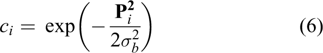
After the fused feature energy is obtained, Gaussian process regression is used to regress the values corresponding to the ground while rejecting the ones to the obstacles. In Figure 7(c), the blue points represent the initial candidate points, the red ones are the seeds for Gaussian process regression, and the green ones are the estimate values representing the ground. At the sudden changes, the estimate green points try to fit the candidate points but fails, then these outliers are assigned high energy as candidate obstacles by equation (6). So this process can be regarded as a self-adaptation and leads to improve the classification.

Covariance matrix selection

Although the SE covariance is suitable for many situations, the main drawback is that the length scale is constant over the whole input space.⁴¹ Note that the length scale is the key element of the SE covariance matrix, and its main property shows that the Gaussian process will fit the input data tightly when the length scale is small, otherwise loosely. Further, the vision-based methods will also bring uncertainty in 3-D positions of the points which will also affect the accuracy at some extent. In order to modify the length scale automatically by the input data to fit different situations and also take into account the stereo uncertainty, the nonstationary, isotropic covariance matrix proposed by Paciorek and Schervish⁴³ with modified length scale for stereo data is proposed.

Take one segment of the polar grip map for example. The nonstationary, isotropic covariance matrix takes the form as follows

k (r_{i}, r_{j}) = σ_{f}^{2} {(l_{i}^{2})}^{\frac{1}{4}} {(l_{i}^{2})}^{\frac{1}{4}} {(\frac{l_{i}^{2} + l_{j}^{2}}{2})}^{- \frac{1}{2}} exp (- \frac{2 {(r_{i} - r_{j})}^{2}}{l_{i}^{2} + l_{j}^{2}})

where $r_{i}$ represents the polar length of ith point in this segment and $l_{i}$ is the corresponding length scale. The covariance captures the local property of $r_{i}$ and $r_{j}$ by averaging between the two length scales.

Therefore, the length scale $l_{i}$ reflects the characteristics at location $r_{i}$ . A suitable approach is to choose a short length scale at the rough ground while a long length scale at flat ground and also influenced by the depth uncertainty. Thus, if the depth is small, the length scale is mainly determined by the change of the ground, while if the depth is large, the length scale is determined by them both.

In this article, the modified length scale is modeled as follows

l_{i} = λ \cdot (a \cdot z_{err} + log (\frac{q}{c_{i}^{2}}))

where a is a scale factor to balance the numeric issue between the stereo depth uncertainty and the cost value which is set as a = 10 in this article, and λ is a scale factor as well, $c_{i}$ is the cost value calculated from the fused features, and $z_{err}$ is the stereo uncertainty⁴⁴ which is modeled as follows

z_{err} = | \frac{z^{2} \cdot D_{err}}{B \cdot F - z \cdot D_{err}} |

where $D_{err}$ is the disparity uncertainty and B and F are the baseline and focal length, respectively. This equation shows that depth uncertainty almost increases quadratically in terms of the distance.

Note that covariance matrix has a variety of types as long as it is reasonable and the covariance matrix is to be positive defined.⁴¹ This proposed matrix works well to represent the relationship between the length scale and the characteristics as discussed above. The next step is to seek the solution of the hyperparameters of the covariance matrix.

Learning geometric hyperparameters

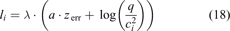
As “Covariance matrix selection” section discussed, the nonstationary covariance matrix has the advantages over the stationary one but needs to be modified due to the vision uncertainty introduced. Equations (17) and (18) provide a feasible model to take into account the vision uncertainty in length scale. However, the hyperparameters $θ = {λ, σ_{f}^{2}, σ_{n}^{2}}$ are unknown and need to be determined. Although the length scale is modified, the optimization method in equation (2) is also suitable in this article.

Given a set of training data $D = {r^{m}, c^{m}}_{m = 1}^{M}$ , where M is the total number of the segments, $r^{m} = {r_{1}^{m}, \dots, r_{n}^{m}}$ is the set of n polar lengths in segment m and $c^{m} = {c_{1}^{m}, \dots, c_{n}^{m}}$ is the corresponding feature fusion cost value set in this segment. Assuming each element to be conditionally independent, the task is to maximizing the pseudo log marginal likelihood⁴¹ as follows

\begin{array}{l} \sum_{m = 1}^{M} log p (c^{m} | r^{m}, θ) \\ = - \frac{1}{2} \sum_{m = 1}^{M} (c^{m}) K_{m}^{- 1} c^{m} - \frac{1}{2} log (\prod_{m = 1}^{M}) | K_{m} | \\ - \frac{log 2 π}{2} \sum_{m = 1}^{M} n_{m} \end{array}

where $K_{m}$ is the covariance matrix for the input $c^{m}$ in segment m and can be calculated by equation (11).

Therefore, compute the partial derivatives of the pseudo log marginal likelihood with respect to the hyperparameters to seek the feasible values as follows

\frac{\partial}{\partial θ} (\sum_{m = 1}^{M} log p (c^{m} | r^{m}, θ)) = \frac{1}{2} \sum_{m = 1}^{M} t r ((α_{m} α_{m}^{T} - K_{m}^{- 1}) \frac{\partial K_{m}}{\partial θ})

where $t r (\cdot)$ is the trace of the matrix, $α_{m} = K_{m}^{- 1} c_{m}$ , and $\frac{\partial K_{m}}{\partial θ_{i}}$ is derivative of a matrix with respect to the parameter as below

\begin{array}{l} \frac{\partial K_{m} (r_{i}, r_{j})}{\partial σ_{f}} = 2 σ_{f} \cdot A \cdot exp (- \frac{2 {(r_{i} - r_{j})}^{2}}{λ^{2} (d_{i}^{2} + d_{j}^{2})}) \\ \frac{\partial K_{m} (r_{i}, r_{j})}{\partial λ} = σ_{f}^{2} \cdot A \cdot exp (- \frac{2 {(r_{i} - r_{j})}^{2}}{λ^{2} (d_{i}^{2} + d_{j}^{2})}) (\frac{4 {(r_{i} - r_{j})}^{2}}{λ^{3} (d_{i}^{2} + d_{j}^{2})}) \\ \frac{\partial K_{m} (r_{i}, r_{j})}{\partial σ_{n}} = 2 σ_{n} δ_{i j} \end{array}

where $A = (d_{i}^{2})^{\frac{1}{4}} {(d_{j}^{2})}^{\frac{1}{4}} {(\frac{d_{i}^{2} + d_{j}^{2}}{2})}^{- \frac{1}{2}}$ and $d_{i} = a \cdot z_{err} + log (\frac{1}{\sqrt{c_{i}}})$ with a = 10 as discussed in “Covariance matrix selection” section.

As there are few labeled free space detection data sets for vision, the KITTI-road detection data set (4) is used. Actually Gaussian process regression is very robust to the parameters so that a few training data are enough to get a feasible result. In this article, three images from each scene are randomly selected as training data for Gaussian process regression to learn the hyperparameters. Finally, the obtained parameters are $θ = {λ, σ_{f}^{2}, σ_{n}^{2}} = {0.1268, 0.0618, 0.0496}$ .

Considering the number of the training images for Gaussian process regression is relatively small to the whole training image set provided by KITTI, testing on training data including the nine images for integrity consideration will have little influence on the performance.

CRF fusion

As Figure 3 shows, the Gaussian process regression will produce the energy-like output. However, incorrect detection is inevitable such as holes or false detection. In order to make the final result more robust and smooth, conditional random field is used which has been very popular in computer vision community. For free space detection, the final result can be regarded as a two-class classification problem (traversable and non-traversable) for each point. In addition, the method in this article focuses more on geometry features so that the constrains in CRF include not only the color information as usual but also the geometry information.

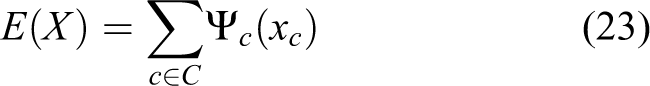
Given a set of pixels $X = {x_{1}, \dots, x_{n}}$ , each pixel $x_{i}$ is modeled with a discrete random variable $l_{i} \in {traversable, non-traversable}$ as its label. The CRF aims to seek an energy minimum configuration of all the labels which equals to minimize the energy model as equation (23) shows

E (X) = \sum_{c \in C} Ψ_{c} (x_{c})

where C is the set of all cliques, $Ψ_{c}$ is the potential function of clique c, and $x_{c}$ is the clique of element x which often takes the format as four-connected or eight-connected neighborhood.

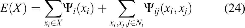
Usually, the potential function $Ψ_{c}$ uses the pairwise style which combines unary potential and pairwise potential as follows

E (X) = \sum_{x_{i} \in X} Ψ_{i} (x_{i}) + \sum_{x_{i}, x_{j}, j \in N_{i}} Ψ_{i j} (x_{i}, x_{j})

where $N_{i}$ is the neighbors of $x_{i}$ and $Ψ_{i j} (x_{i}, x_{j})$ is the pairwise potential relative to $x_{i}$ .

Similarly as the mapping in equation (20), the unary potential $Ψ_{i} (x_{i})$ takes the negative log cost energy $d (x_{i})$ from Gaussian process regression as the form $Ψ_{i} (x_{i}) = - log (d (x_{i}))$ which is nontrivial because this mapping widens the margin between the two classes and benefits the CRF inference.

Usually, the pairwise potential is quite important and most works take into account the color consistency. In this article, the pairwise potential also considers the geometry constrains. Thus, the pairwise potential takes the form as follows

Ψ_{i j} (x_{i}, x_{j}) = Ψ_{i j}^{c} (x_{i}, x_{j}) + Ψ_{i j}^{g} (x_{i}, x_{j})

where $Ψ_{i j}^{c} (x_{i}, x_{j})$ represents the color consistency constrain on penalizing the neighboring pixels which take different labels. As it is in the study by Rother et al.,⁴⁵ the pairwise potential takes the form as follows

Ψ_{i j}^{c} (x_{i}, x_{j}) = {\begin{array}{l} 0, & x_{i} = x_{j} \\ λ_{1} \frac{1}{dist (i, j)} \cdot exp (- \frac{∥ I_{i} - I_{j} ∥^{2}}{2 β}), & otherwise, \end{array}

where $I_{i}$ is the RGB values of the pixel $x_{i}$ , $dist (i, j)$ is the Euclidean distance between the neighboring pixels i and j in eight-connected fashion, β is the expectation of the square contrast over the whole image, and $λ_{1}$ is the parameter for trade-off between the pairwise terms.

$Ψ_{i j}^{g} (x_{i}, x_{j})$ represents the geometry constrain on rewarding the neighboring points which take different labels because the different geometry property makes the labels different. In this article, the geometry constrain takes the similar form as color constrain as follows

\begin{array}{l} Ψ_{i j}^{g} (x_{i}, x_{j}) = - λ_{2} \\ {\begin{array}{l} 0, & x_{i} = x_{j} \\ max (0, cos t (i, j) exp (- \frac{∥ N_{i} \oplus N_{j} ∥^{2}}{2 σ_{g}^{2}})), & otherwise \end{array} \end{array}

where $cos t (i, j) = log (1 + \frac{1}{dist (i, j)})$ , $N_{i}$ is the normal to the tangent surface at the 3-D location with respect to pixel $x_{i}$ , ⊕ is the operation which returns the angle between two vectors, $σ_{g}$ is the standard variance which equals to the normal variance in equation (8), and $λ_{2}$ is also the parameter for trade-off.

In Figure 8, it shows the pairwise constrains of color information and geometry information.

Figure 8.

Pairwise constrains displayed in images. The first row from (a) to (d) shows the pairwise constrains of color information which correspond to horizental, northwest, southwest, and vertical direction in image space, respectively. The bottom row from (e) to (h) shows the counterparts of geometry constrains.

Experiments and discussion

Experiment settings

Basically, the experiments are tested on a laptop with 16 GB RAM and single Intel Core i5-6300HQ with 2.3 GHz. The algorithm was implemented with C++ under Ubuntu14.04. The parameters of the proposed algorithm are mainly set for stereo matching, feature fusion, Gaussian process regression, and conditional random field inference. Note that the parameters of feature fusion and GPR are introduced in the corresponding “Gaussian process regression” and “Bayesian-based multiple feature fusion framework” sections. Others will discussed in the following. Table 1 briefly shows the time-consuming in each step in our proposed algorithm. Since it is not well optimized, the average computation time-consuming is about 30 s for each frame. However, it is possible to accelerate by parallel or GPU computation.

Table 1.

Time-consuming by steps.

Method	Time-consuming (s)
Stereo matching	2
Features computation (mainly normals)	25
Gaussian process regression	0.1
CRF inference	1

For the parameter selection in stereo algorithm, our goal is to obtain a smooth depth map but still details remained as much as possible. In order to find a proper parameter set, the previous algorithm which only exploits the height feature is used. Figure 9 shows the comparison on MaxF scores with respect to the number of superpixels. More superpixels will keep more details theoretically, but probably make the depth map unsolvable and consume much more time. Therefore, 8000 superpixels are chosen and the smoothness is set to 10 experimentally.

Figure 9.

MaxF scores with respect to the number of superpixels.

Data sets

In order to valid the approach proposed in this article, quantitative and qualitative experiments are tested on two different data sets. One is the KITTI-road (4) for quantitative test as a reference. Another is our own campus data set for qualitative test.

The KITTI-road data set benchmark contains 289 training and 290 testing pairs of images with calibrated parameters which includes three categories (both for training/testing): UU-urban unmarked (98/100), UM-urban marked (95/96), and UMM-urban multiple marked lanes (96/94). See equation (4) for details. As the lane detection is the special case, the test in this article only focuses on the road detection and adopts the metrics in pixel-wise as in KITTI benchmark for its training data set and testing data set.

The campus data set contains an amount of pairs of synchronized images in campus scene. Although the scenes in this data set are not complex, they are different in light condition and color distribution compared to KITTI data set.

Baseline

In order to show the improvement of this approach compared to typical free space detection algorithms, the method in previous work (2) is changed into vision-based version called Height+GPR, and the method in equation (9) is implemented called Stixel for comparison. Although the performance perhaps decreases due to the different implementation, the comparison will show the significant improvement.

At the same time, other similar methods in KITTI-road are also compared for reference including HistonBoost,⁴⁶ BL,⁴ RES3D-Stereo,¹⁷ and BM.⁴⁷ In order to compare a learning-based method, a subpart of the method in equation (20) called ColorBoost is used as an example.

Quantitative result on KITTI data set

In this part, three comparisons are tested.

MultiFeat+CRF versus MultiFeat+GPR+CRF

To valid the improvement of Gaussian process regression, the methods with and without this process are compared. One applies fused multiple features directly combined with CRF which is named MultiFeat+CRF for short. The other applies Gaussian process regression after the multiple feature fusion which is named MultiFeat+GPR+CRF. At the same time, a set of experiments on comparing the CRF parameters $λ_{1}$ and $λ_{2}$ are also taken.

As the metric MaxF comes in the first place in KITTI-road ranking, the comparison mainly focuses on this parameter. Figure 10 illustrates a set of comparisons on three different scenes of KITTI-road with different CRF parameter pairs. In this figure, it is obvious that one with Gaussian process regression outperforms the counterpart which is without this process.

Figure 10.

MultiFeat+CRF and MultiFeat+GPR+CRF for MaxF result on training data set with different CRF parameter pairs.

In the methods with Gaussian process regression, the performances will gradually rise up when geometry constrain parameter $λ_{2}$ increases until the parameter pair arrives at about $λ_{1} = 20$ and $λ_{2} = 5$ , reaching a relative peak. Although the metric value of $λ_{2} = 10$ in UU_road scene still rises up, the best choice is still the parameter pair as mentioned considering the entire performance of the three scenes as a whole. Therefore, this parameter pair is set as the best pair on the training data set and is used for the following experiments. Note that the quantitative results may have a bias due to the different definitions of free space and road detection but they can show the average ability of detection on KITTI-road data set at some extent.

$λ_{1}$ and $λ_{2}$ in equations (26) and (27) are used in trade-off the values of the color and geometry constrains, respectively, in CRF. Figure 11 shows comparisons on the effect of free space detection by different constrain parameters. Recall that color constrain tries to merge the regions with similar color intensities while geometry constrain tries to keep the sudden change regions with different geometry features. In this example, because of the noise in the middle of image in Figure 11(a), the free space in this direction is stopped but the color similarity around that point is very strong, thus larger value of color constrain makes CRF merge these holes and improves the performance in Figure 11(b). In terms of geometry constrain, large geometry constrain in Figure 11(d) makes it more accurate at the edge of the road compared to the result in Figure 11(c).

Figure 11.

Comparison on CRF parameters showing the property of color and geometry constrains.

MultiFeat+GPR+CRF fuses pre-trained color and context classifier

The algorithm in this work mainly focuses on geometry features, while in order to show that it is flexible to add new features to improve the performance, the color and context features trained by boosted trees in equation (20) are introduced in the fusion framework. The improvement by new feature is shown in Figure 12 where the color and context information makes the first sudden change on the left at the boundary between road and medium grass rises up significantly in Figure 12(e) compared to that in Figure 12(d) without this additional feature, thus enhances the classification result.

Figure 12.

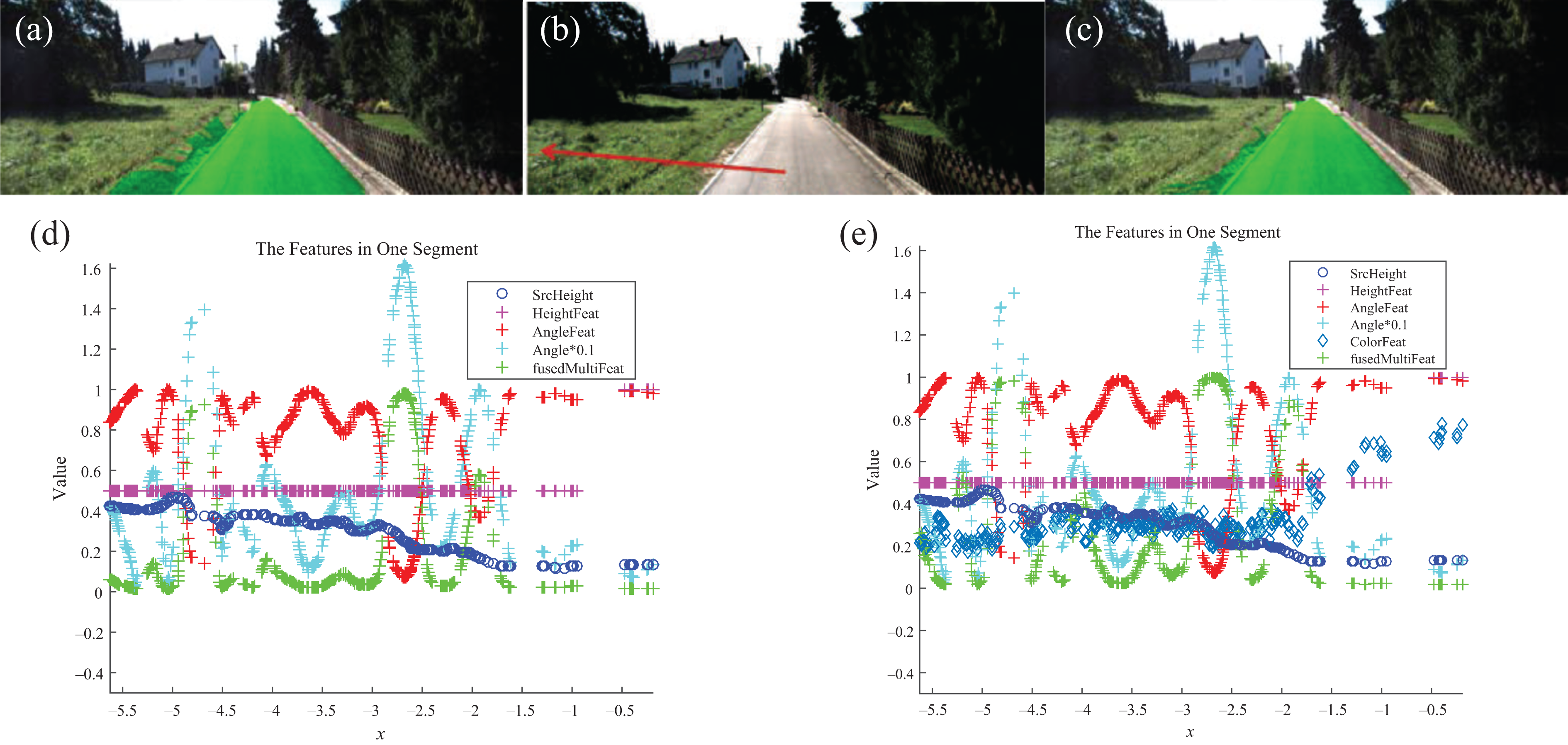
Additional color and context feature enhances the classification result. (b) The original image with the specified segment in red. (a) and (c) The detection results with respect to the methods with and without additional color feature. (d) and (f) The corresponding details of the features in this segmentation. The new added feature improves the energy (in green) of the free-space estimates.

The metric results for KITTI-road training data set are provided in Tables 2 to 7. In these tables, this proposed algorithm shows a competitive results on the training data set both on perspective view and BEV.

Table 2.

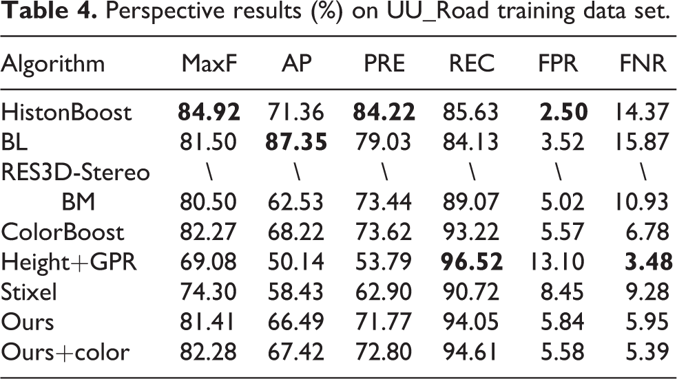
Perspective results (%) on UM_Road training data set.

Algorithm	MaxF	AP	PRE	REC	FPR	FNR
HistonBoost	90.58	83.47	90.20	90.96	1.90	9.04
BL	89.62	93.21	89.32	89.93	2.12	10.07
RES3D-Stereo	\	\	\	\	\	\
BM	85.67	72.21	77.83	95.26	5.18	4.74
ColorBoost	88.62	76.95	83.00	95.06	3.82	4.94
Height+GPR	71.94	53.31	56.99	97.52	14.51	2.48
Stixel	73.86	57.01	61.06	93.46	11.75	6.54
Ours	87.23	75.32	81.20	94.23	4.30	5.77
Ours+color	88.77	77.29	83.37	94.91	3.73	5.09

Table 3.

Perspective results (%) on UMM_Road training data set.

Algorithm	MaxF	AP	PRE	REC	FPR	FNR
HistonBoost	88.72	78.45	83.92	94.11	5.62	5.89
BL	83.00	89.42	77.65	89.14	8.03	10.86
RES3D-Stereo	\	\	\	\	\	\
BM	88.76	81.29	87.04	90.55	4.20	9.45
ColorBoost	91.29	82.17	87.95	94.89	4.18	5.11
Height+GPR	82.74	67.87	72.28	96.73	11.62	3.27
Stixel	84.23	71.72	76.50	93.68	9.01	6.32
Ours	92.56	84.47	90.53	94.67	3.10	5.33
Ours+color	93.25	85.32	91.46	95.10	2.78	4.90

Comparisons to other methods

In order to evaluate the performance of the proposed algorithm (ours is short for Geo + GPR + CRF and ours + color for Geo + Color+ GPR + CRF), a set of comparisons on KITTI-road data set are taken including HistonBoost,⁴⁶ BL,⁴ RES3D-Stereo,¹⁷ BM,⁴⁷ and ColorBoost.²⁰ Tables 2 to 4 show the perspective view comparisons to other methods on training data set, while Tables 5 to 7 are for BEV comparisons. Note that the results are evaluated on the latest version of ground truth, while the results in HistonBoost,⁴⁶ RES3D-Stereo,¹⁷ and BM⁴⁷ are from the corresponding literatures. Some of them may be evaluated on old version criteria but they will not vary dramatically.

Table 4.

Perspective results (%) on UU_Road training data set.

Algorithm	MaxF	AP	PRE	REC	FPR	FNR
HistonBoost	84.92	71.36	84.22	85.63	2.50	14.37
BL	81.50	87.35	79.03	84.13	3.52	15.87
RES3D-Stereo	\	\	\	\	\	\
BM	80.50	62.53	73.44	89.07	5.02	10.93
ColorBoost	82.27	68.22	73.62	93.22	5.57	6.78
Height+GPR	69.08	50.14	53.79	96.52	13.10	3.48
Stixel	74.30	58.43	62.90	90.72	8.45	9.28
Ours	81.41	66.49	71.77	94.05	5.84	5.95
Ours+color	82.28	67.42	72.80	94.61	5.58	5.39

Table 5.

BEV results (%) on UM_Road training data set.

Algorithm	MaxF	AP	PRE	REC	FPR	FNR
HistonBoost	\	\	\	\	\	\
BL	81.34	86.42	77.09	86.09	11.76	13.91
RES3D-Stereo	74.50	75.74	65.75	85.93	18.79	14.07
BM	\	\	\	\	\	\
ColorBoost	\	\	\	\	\	\
Height+GPR	66.49	49.10	53.01	89.15	36.34	10.85
Stixel	61.95	47.59	56.79	68.15	23.84	31.85
Ours	80.93	68.30	76.48	85.93	12.15	14.07
Ours+color	82.79	70.11	78.69	87.35	10.88	12.65

BEV: bird eye view.

Table 6.

BEV results (%) on UMM_Road training data set.

Algorithm	MaxF	AP	PRE	REC	FPR	FNR
HistonBoost	\	\	\	\	\	\
BL	79.48	84.04	72.83	87.47	35.59	12.53
RES3D-Stereo	82.78	86.07	84.37	81.25	15.60	18.75
BM	\	\	\	\	\	\
ColorBoost	\	\	\	\	\	\
Height+GPR	79.80	69.67	71.42	90.40	39.45	9.60
Stixel	75.28	67.11	72.71	78.05	31.95	21.95
Ours	88.16	82.53	85.56	90.92	16.73	9.08
Ours+color	88.80	82.90	85.97	91.81	16.34	8.19

BEV: bird eye view.

Table 7.

BEV results (%) on UU_Road training data set.

Algorithm	MaxF	AP	PRE	REC	FPR	FNR
HistonBoost	\	\	\	\	\	\
BL	73.02	76.96	68.57	78.10	12.74	21.90
RES3D-Stereo	74.49	70.71	71.49	77.75	10.53	22.25
BM	\	\	\	\	\	\
ColorBoost	\	\	\	\	\	\
Height+GPR	68.08	50.24	55.57	87.85	24.99	12.15
Stixel	63.72	51.36	65.71	61.85	11.49	38.15
Ours	78.70	65.46	74.18	83.80	10.38	16.20
Ours+color	79.87	66.18	75.05	85.35	10.10	14.65

BEV: bird eye view.

Figure 13 illustrates some typical comparison results on the training data set. The proposed method is compared to the baseline Stixel and Height+GPR, demonstrating inspiring improvement.

Figure 13.

Comparison results on training data set. The first column shows row by row the original image and the road ground truth. The second column shows the corresponding results of our proposed method. The third column shows the Gaussian process regression results-based height feature while the last column shows the results of stixel-based method.

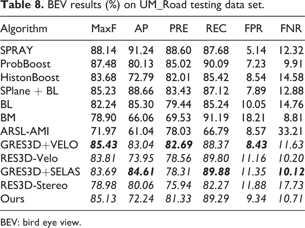
For online testing on KITTI road detection, Figure 14 illustrates some testing results for both BEV and perspective view. Tables 8 to 11 show comparisons of some relevant methods. In the ranking list online, it can be seen that the learning-based methods outperform others significantly, especially the approaches based on deep networks achieve almost perfect scores. However, these methods have potential risk in other inexperienced scenes. On the contrary, the method proposed in this article mainly relies on geometry information which makes it to be versatile to various scenes and is also compatible to learning-based methods due to the flexible fusion framework which makes it easy to be improved. In spite of the outstanding learning-based methods in the ranking list, our approach is competitive and promising. When compared to the methods based on only stereo and geometry information, ours can be regarded as the best one, being better than RES3D-Stereoand GRES3D+SELAS and even comparable to their upgraded Lidar-based versions GRES3D+VELO and RES3D-Velo. The relevant results are highlighted by bold italic in these tables which are typically regarded as geometry-based approaches. Note that Lidar point data will definitely improve the performance through precise 3-D structures.

Figure 14.

Online testing results. The first row shows the BEV and the second row shows the corresponding perspective results. The color encodes green for truth positive, blue for false positive, and red for false negative. BEV: bird eye view.

Table 8.

BEV results (%) on UM_Road testing data set.

Algorithm	MaxF	AP	PRE	REC	FPR	FNR
SPRAY	88.14	91.24	88.60	87.68	5.14	12.32
ProbBoost	87.48	80.13	85.02	90.09	7.23	9.91
HistonBoost	83.68	72.79	82.01	85.42	8.54	14.58
SPlane + BL	85.23	88.66	83.43	87.12	7.89	12.88
BL	82.24	85.30	79.44	85.24	10.05	14.76
BM	78.90	66.06	69.53	91.19	18.21	8.81
ARSL-AMI	71.97	61.04	78.03	66.79	8.57	33.21
GRES3D+VELO	85.43	83.04	82.69	88.37	8.43	11.63
RES3D-Velo	83.81	73.95	78.56	89.80	11.16	10.20
GRES3D+SELAS	83.69	84.61	78.31	89.88	11.35	10.12
RES3D-Stereo	78.98	80.06	75.94	82.27	11.88	17.73
Ours	85.13	72.24	81.33	89.29	9.34	10.71

BEV: bird eye view.

Table 9.

BEV results (%) on UMM_Road testing data set.

Algorithm	MaxF	AP	PRE	REC	FPR	FNR
SPRAY	89.69	93.84	89.13	90.25	12.10	9.75
ProbBoost	91.36	84.92	88.18	94.78	13.97	5.22
HistonBoost	88.73	81.57	84.49	93.42	18.85	6.58
SPlane + BL	82.04	85.56	75.11	90.39	32.93	9.61
BL	76.02	78.82	65.71	90.17	51.72	9.83
BM	89.41	80.61	83.43	96.30	21.02	3.70
ARSL-AMI	89.56	82.82	85.87	93.59	16.93	6.41
GRES3D+VELO	88.19	88.65	83.98	92.85	19.48	7.15
RES3D-Velo	90.60	85.38	85.96	95.78	17.20	4.22
GRES3D+SELAS	87.57	90.52	85.92	89.28	16.08	10.72
RES3D-Stereo	83.62	85.74	79.81	87.81	24.42	12.19
Ours	88.20	82.33	85.32	91.27	17.26	8.73

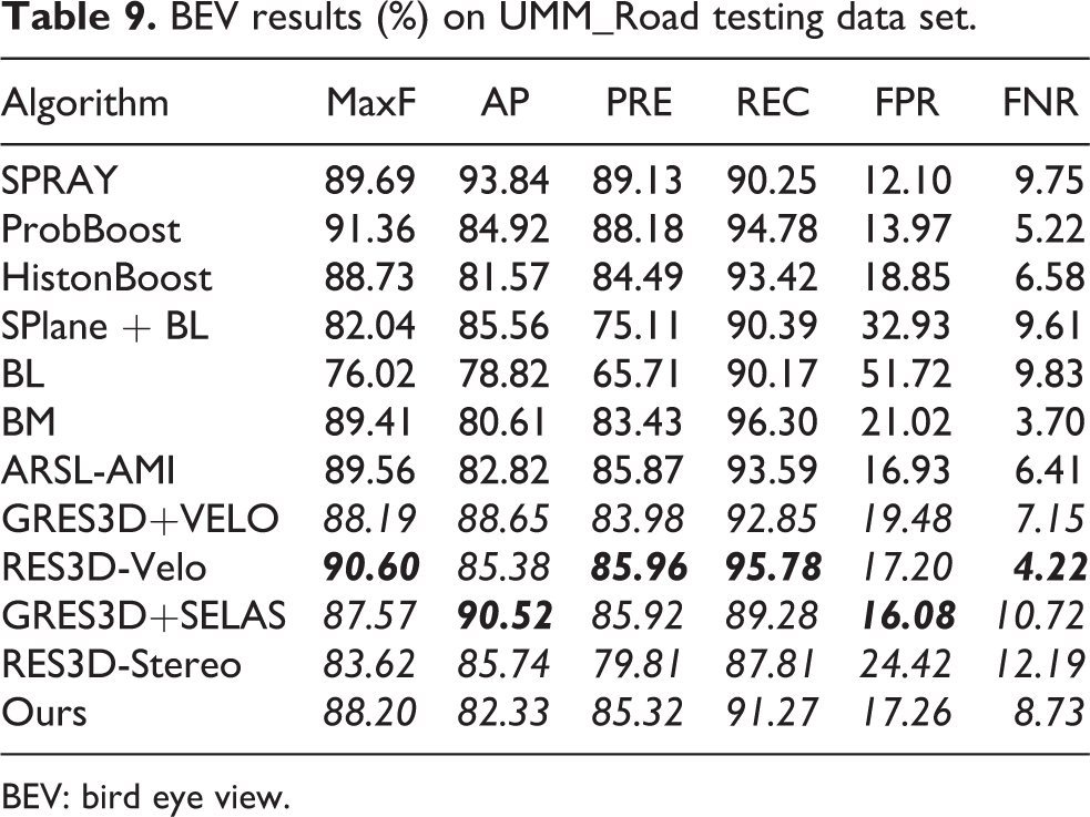
BEV: bird eye view.

Table 10.

BEV results (%) on UU_Road testing data set.

Algorithm	MaxF	AP	PRE	REC	FPR	FNR
SPRAY	82.71	87.19	82.16	83.26	5.89	16.74
ProbBoost	80.76	68.70	85.25	76.72	4.33	23.28
HistonBoost	74.19	63.01	77.43	71.22	6.77	28.78
SPlane + BL	74.02	79.61	65.15	85.68	14.93	14.32
BL	69.50	73.87	65.87	73.56	12.42	26.44
BM	78.43	62.46	70.87	87.80	11.76	12.20
ARSL-AMI	70.33	61.97	83.33	60.84	3.97	39.16
GRES3D+VELO	84.14	80.20	80.57	88.03	6.92	11.97
RES3D-Velo	83.63	72.58	77.38	90.97	8.67	9.03
GRES3D+SELAS	82.70	83.95	78.54	87.32	7.77	12.68
RES3D-Stereo	78.75	73.60	77.63	79.90	7.50	20.10
Ours	81.00	69.74	79.78	82.27	6.79	17.73

BEV: bird eye view.

Table 11.

BEV results (%) on Urban_Road testing data set.

Algorithm	MaxF	AP	PRE	REC	FPR	FNR
SPRAY	87.09	91.12	87.10	87.08	7.10	12.92
ProbBoost	87.78	77.30	86.59	89.01	7.60	10.99
HistonBoost	83.92	73.75	82.24	85.66	10.19	14.34
SPlane + BL	79.63	83.90	72.59	88.17	18.34	11.83
BL	75.80	79.85	69.31	83.63	20.40	16.37
BM	83.47	72.23	75.90	92.72	16.22	7.28
ARSL-AMI	80.36	70.23	83.24	77.67	8.61	22.33
GRES3D+VELO	86.07	84.34	82.16	90.38	10.81	9.62
RES3D-Velo	86.58	78.34	82.63	90.92	10.53	9.08
GRES3D+SELAS	85.09	86.86	82.27	88.10	10.46	11.90
RES3D-Stereo	81.08	81.68	78.14	84.24	12.98	15.76
Ours	85.56	74.21	82.81	88.50	10.12	11.50

BEV: bird eye view.

Qualitative result on our own campus data set

To valid the versatility of this proposed method on other data set, our own campus data set is used for qualitative evaluation. For comparison, the color and context-based learning method ColorBoost in equation (20) is used. The metric scores in Tables 2 to 4 for KITTI-road test show its excellent performance. However, this pre-trained model on KITTI-road data set performs not appealing in our own campus data set. Although it returns good results in some scenarios which are similar to one of the pre-trained scenes as shown in the fourth row in Figure 15, it perhaps reflects at some extent that this learning-based method cannot work well on other different scenes, which is shown in the first to third rows. This also proves that the proposed geometry-based approach is robust and need not retrain on different scenes.

Figure 15.

Some comparisons on our own campus data set. The first to forth columns are the results of ours proposed method in this article, the UM_Road color model, the UMM_Road color model, and the UU_Road color model, respectively.

Discussion on the results

Although the quantitative evaluation scores are behind the outstanding learning-based methods especially the ones with deep networks, the results of the proposed method can be considered very satisfactory and inspiring when compared to other excellent methods in the literature. And it can be regarded as a geometry-based method which is very versatile to many other scenarios. However, there are still some reasons limiting the improvement.

Criteria

Recall that our method aims at free space detection of which the criteria are little different from that of road detection. This can be illustrated in some typical situations shown in Figure 16. In image Figure 16(a), the path to the right passage is obvious traversable so that this region is classified as free space reasonably while the ground truth of road detection Figure 16(b) considers this region is non-road because seldom will a vehicle drive into this path. Similarly, although there is a small curb between the road and the parking place shown in Figure 16(c), yet it is too small to prevent the vehicle, resulting that the free space detection returns a high false positive rate which will cause decrease in the final metric scores. Another typical situation is shown in Figure 16(e). The left space of the left car is non-traversable because this car stops the way, thus it is not practical to go through it. For this reason, it is impossible to correctly classify this area as road under this criteria for free space detection methods while road detection methods will take this region into account as road which shows the ground truth in Figure 16(f).

Figure 16.

Different criteria make the results different. The left column shows the free space detection results by our algorithm and the right column provides the corresponding ground truth in KITTI-road data set.

Actually, for autonomous vehicles, free space or road detection task aims at path planning. A successful path planning is made by a set of factors which are certainly different from the metrics here. Therefore, it perhaps does not affect the path planning results no matter what types of some area are classified. If so, the evaluation metrics from path planning may be another more reasonable criteria.

Stereo accuracy

Although the approach in equation (35) provides a state-of-the-art dense depth estimate method, the slanted plane model still modifies the scenes at the sudden changes and forces them tend to be smooth. As a result, this inevitably degenerates the accuracy. Despite of this effect, the stereo matching sometimes fails due to the variations of light condition and shadow effects. These issues will consequentially occur fatal errors, as can be seen in Figure 17(a) where the disparity map in the first row returns wrong matchings, causing a terrible failure. Additionally, due to the limit of stereo algorithm, the accuracy of distant points falls down so that the detection will return false results (see the left edge of the free space detection in the distance). This can be demonstrated in Figure 17(b).

Figure 17.

Failure modes due to the failure of stereo matching and excess of stereo smoothing.

Features

Despite the satisfactory results obtained, the geometry features in this article are very simple. However, the flexible feature fusion framework ensures it extendable to more features which has been proved by the experiment that additional color and context information improves the performance. So more powerful features can definitely enhance the detection results.

Conclusions and future work

In this article, a robust geometry-based free space detection method is proposed which resolves some remain issues. The fusion framework is flexible to extend and Gaussian process regression automatically improves the energy distribution which both help conditional random field to achieve a better classification. This method avoids several common assumptions that is free to general scenes. In order to evaluate the approach, a set of experiments are tested on the popular KITTI-road data set for quantitative comparisons and our own campus data set for qualitative comparisons. The method returns satisfactory and inspiring performance on the free space detection compared to other outstanding approaches in multiple scenes without previous training and assumptions about road geometry. The performance is even competitive to some relevant Lidar-based methods.

As for the future work, in order to obtain a better 3-D environment modeling, methods for accurate 3-D measurement and more robust features are required as well as solutions for the light condition variation and occlusion. Also, Simultaneous Localization and Mapping (SLAM) based local mapping techniques will help to improve the understanding of the environment significantly and result in better free space detection.

Footnotes

Declaration of conflicting interests

The author(s) declared no potential conflicts of interest with respect to the research, authorship, and/or publication of this article.

Funding

The author(s) disclosed receipt of the following financial support for the research, authorship, and/or publication of this article: The work is support by National Nature Science Foundation of China under Grant No. 61375050 and Grant No. 91220301, and ARC Discovery grants: DP120103896, DP130104567, and CE140100016. The first author is funded by the Chinese Scholarship Council (CSC) to be a joint PhD student from NUDT to ANU. We would like to thank the anonymous reviewers for their valuable comments.

References

Geiger

Lenz

Stiller

. Vision meets robotics: the KITTI data set. Int J Robot Res 2013; 32(11): 1231–1237.

Chen

Dai

Wang

. Gaussian-process-based real-time ground segmentation for autonomous land vehicles. J Intell Robot Syst 2014; 76(3-4): 563–582.

Chen

Dai

Liu

. Velodyne-based curb detection up to 50 m away. In: 2015 IEEE intelligent vehicles symposium (IV), Seoul, South Korea, 28 June–1 July 2015, pp. 241–248. IEEE.

Fritsch

Kuehnl

Geiger

. A new performance measure and evaluation benchmark for road detection algorithms. In: 16th International IEEE conference on intelligent transportation systems (ITSC 2013), The Hague, Netherlands, 6–9 October 2013, pp. 1693–1700. IEEE.

Badino

Franke

Mester

. Free space computation using stochastic occupancy grids and dynamic programming. In: Workshop on dynamical vision, ICCV, Rio de Janeiro, Brazil, 14–20 October 2007, Vol. 20.

Labayrade

Aubert

Tarel

. Real time obstacle detection in stereovision on non-flat road geometry through” v-disparity” representation. In: Intelligent vehicle symposium, 2002. IEEE, Versailles, France, France, 17–21 June 2002, Vol. 2, pp. 646–651. IEEE.

Caraffi

Cattani

Grisleri

. Off-road path and obstacle detection using decision networks and stereo vision. IEEE Trans Intell Transp Syst 2007; 8(4): 607–618.

Santana

Santos

Correia

. Cross-country obstacle detection: space-variant resolution and outliers removal. In: 2008 IEEE/RSJ international conference on intelligent robots and systems, IEEE, pp. 1836–1841.

Badino

Franke

Pfeiffer

. The stixel world-a compact medium level representation of the 3D-world. In: Joint pattern recognition symposium. Springer, 2009, pp. 51–60.

10.

Oniga

Nedevschi

Meinecke

. Road surface and obstacle detection based on elevation maps from dense stereo. In: 2007 IEEE intelligent transportation systems conference, Seattle, WA, USA, 30 September–3 October 2007, pp. 859–865. IEEE.

11.

Oniga

Nedevschi

. Processing dense stereo data using elevation maps: road surface, traffic isle, and obstacle detection. IEEE Trans Veh Technol 2010; 59(3): 1172–1182.

12.

Coué

Pradalier

Laugier

. Bayesian occupancy filtering for multitarget tracking: an automotive application. Int J Robot Res 2006; 25(1): 19–30.

13.

Tay

Mekhnacha

Chen

. An efficient formulation of the Bayesian occupation filter for target tracking in dynamic environments. Int J Veh Auton Syst 2008; 6(1-2): 155–171.

14.

Wedel

Badino

Rabe

. B-spline modeling of road surfaces with an application to free-space estimation. IEEE Trans Intell Transp Syst 2009; 10(4): 572–583.

15.

Manduchi

Castano

Talukder

. Obstacle detection and terrain classification for autonomous off-road navigation. Auton Robot 2005; 18(1): 81–102.

16.

Mendes

CCT

Fremont

Wolf

. Exploiting fully convolutional neural networks for fast road detection. In: Robotics and Automation (ICRA), 2016 IEEE International Conference on, Stockholm, Sweden, 16–21 May 2016, pp. 3174–3179. IEEE.

17.

Shinzato

Gomes

Wolf

. Road estimation with sparse 3D points from stereo data. In: 17th international IEEE conference on intelligent transportation systems (ITSC), Qingdao, China, 8–11 October 2014, pp. 1688–1693. IEEE.

18.

Shinzato

Wolf

DF,

Stiller

. Road terrain detection: avoiding common obstacle detection assumptions using sensor fusion. In: 2014 IEEE intelligent vehicles symposium proceedings, Dearborn, MI, USA, 8–11 June 2014, pp. 687–692. IEEE.

19.

Kühnl

Kummert

Fritsch

. Spatial ray features for real-time ego-lane extraction. In: 2012 15th International IEEE conference on intelligent transportation systems, Anchorage, AK, USA, 16–19 September 2012, pp. 288–293. IEEE.

20.

Xiao

Dai

Liu

. CRF based road detection with multi-sensor fusion. In: 2015 IEEE intelligent vehicles symposium (IV), Seoul, South Korea, 28 June–1 July 2015, pp. 192–198. IEEE.

21.

Xiao

Dai

Liu

. Monocular road detection using structured random forest. Int J Adv Robot Syst 2016; 13(3): 101.

22.

Xiao

Wang

Dai

. Hybrid conditional random field based camera-Lidar fusion for road detection. Inf Sci 2017. Elsevier.

23.

Lin

Shen

Hengel

AVD

, et al. Efficient piecewise training of deep structured models for semantic segmentation. In: Proceedings of the IEEE Conference on Computer Vision and Pattern Recognition, Las Vegas, NV, USA, 27–30 June 2016, pp. 3194–3203.

24.

Siegemund

Pfeiffer

Franke

. Curb reconstruction using conditional random fields. In: Intelligent vehicles symposium (IV), 2010 IEEE, IEEE, pp. 203–210.

25.

Siegemund

Franke

Förstner

. A temporal filter approach for detection and reconstruction of curbs and road surfaces based on conditional random fields. In: Intelligent vehicles symposium (IV), 2011 IEEE, Baden-Baden, Germany, 5–9 June 2011, IEEE, pp. 637–642.

26.

Kellne

Hofman

Bouzoura

. Multi-cue, model-based detection and mapping of road curb features using stereo vision. In: 2015 IEEE 18th International conference on intelligent transportation systems, IEEE, pp. 1221–1228.

27.

Oniga

Nedevschi

. Polynomial curb detection based on dense stereovision for driving assistance. In: 2010 13th International IEEE conference on, intelligent transportation systems (ITSC), Funchal, Portugal, 19–22 September 2010, pp. 1110–1115. IEEE.

28.

Lahat

Adali

Jutten

. Multimodal data fusion: an overview of methods, challenges, and prospects. Proc IEEE 2015; 103(9): 1449–1477.

29.

Liu

Guo

Sun

. Object recognition using tactile measurements: kernel sparse coding methods. IEEE Trans Instrum Meas 2016; 65(3): 656–665.

30.

Liu

Sun

Guo

. Structured output-associated dictionary learning for haptic understanding. IEEE Trans Syst Man Cybern Syst 2017; (99): 1–11. DOI: 10.1109/TSMC.2016.2635141.

31.

Liu

Sun

. Visual-tactile fusion for object recognition. IEEE Trans Autom Sci Eng 2017; 14(2): 996–1008.

32.

Liu

Sun

Fang

. Robotic room-level localization using multiple sets of sonar measurements. IEEE Trans Instrum Meas 2017; 66(1): 2–13.

33.

Liu

Qin

Sun

. Extreme kernel sparse learning for tactile object recognition. IEEE Trans Syst Man Cybern 2017: 1–12.

34.

Sutton

McCallum

. An introduction to conditional random fields. Vol. 4(4). Foundations and Trends® in Machine Learning, 2012, pp. 267–373.

35.

Yamaguchi

McAllester

Urtasun

. Efficient joint segmentation, occlusion labeling, stereo and flow estimation. In: European conference on computer vision, Zurich, Switzerland, 6–12 September 2014, pp. 756–771. Springer.

36.

Hirschmuller

. Stereo processing by semiglobal matching and mutual information. In: IEEE Transactions on Pattern Analysis and Machine Intelligence (TPAMI), Portland, OR, USA, 23–28 June 2013, pp. 328–341.

37.

Pfeiffer

Gehrig

Schneider

. Exploiting the power of stereo confidences. In: Proceedings of the IEEE conference on computer vision and pattern recognition, Portland, OR, USA, 23–28 June 2013, pp. 297–304

38.

Rusu

Cousins

. 3D is here: Point cloud library (PCL). In: 2011 IEEE international conference on, robotics and automation (ICRA), Shanghai, China, 9–13 May 2011, pp. 1–4. IEEE.

39.

Bishop

. Pattern recognition. Mach Learn 2006; 128: 1–58.

40.

Piegl

Tiller

. The NURBS book. Springer Science and Business Media, 2012.

41.

Rasmussen

CE.

Gaussian processes in machine learning. In: Advanced lectures on machine learning, Vol. 3176, Springer, 2004. pp. 63–71.

42.

Douillard

Underwood

Kuntz

. On the segmentation of 3D Lidar point clouds. In: 2011 IEEE international conference on, robotics and automation (ICRA), Shanghai, China, 9–13 May 2011, pp. 2798–2805. IEEE.

43.

Paciorek

Schervish

. Nonstationary covariance functions for Gaussian process regression. Adv Neural Inf Process Syst 2004; 16: 273–280.

44.

Oniga

Nedevschi

Meinecke

. Curb detection based on elevation maps from dense stereo. In: 2007 IEEE international conference on intelligent computer communication and processing, IEEE, pp. 119–125.

45.

Rother

Kolmogorov

Blake

. Grabcut: interactive foreground extraction using iterated graph cuts. In: ACM transactions on graphics (TOG), Vol. 23, pp. 309–314. ACM.

46.

Vitor

Victorino

AC,

Ferreira

. Comprehensive performance analysis of road detection algorithms using the common urban KITTI-road benchmark. In: 2014 IEEE intelligent vehicles symposium proceedings, Dearborn, MI, USA, 8–11 June 2014, pp. 19–24. IEEE.

47.

Wang

Frémont

Rodríguez

. Color-based road detection and its evaluation on the KITTI road benchmark. In: 2014 IEEE intelligent vehicles symposium proceedings, Dearborn, MI, USA, 8–11 June 2014, pp. 31–36. IEEE.

Gaussian process regression-based robust free space detection for autonomous vehicle by 3-D point cloud and 2-D appearance information fusion

Abstract

Keywords

Introduction

Related works

System overview

Stereo data acquisition, polar coordinate representation, and feature representation

Stereo data acquisition

Polar coordinate representation

Bayesian-based multiple feature fusion framework

Normal vector feature

Vicinity height feature

Other useful features

Gaussian process regression

Motivation

Brief overview of GP

Gaussian process regression-based cost energy computation

Covariance matrix selection

Learning geometric hyperparameters

CRF fusion

Experiments and discussion

Experiment settings

Data sets

Baseline

Quantitative result on KITTI data set

MultiFeat+CRF versus MultiFeat+GPR+CRF

MultiFeat+GPR+CRF fuses pre-trained color and context classifier

Comparisons to other methods

Qualitative result on our own campus data set

Discussion on the results

Criteria

Stereo accuracy

Features

Conclusions and future work

Footnotes

Declaration of conflicting interests

Funding

References