Thermal matching using Gaussian process regression

Abstract

Thermal matching is a key stage of the development process for a gas turbine engine where component models are verified to ensure the correct metal temperature distribution has been used in life calculations. The thermal match involves adjusting parameters of a thermal model in order to match an experimental temperature distribution, usually obtained from a thermal paint test. Current methodologies involve manually adjusting parameters, which is both time consuming and leads to variation in the matches achieved. This paper presents a new method to conduct thermal matching, where Gaussian process regression is utilised to obtain a surrogate model from which optimal parameters for matching are obtained. This standardised procedure removes subjectivity from the match and gives faster and more consistent matches. The method is introduced and demonstrated for a number of cases involving a leading edge impingement system that has been isolated from a high pressure turbine blade.

Introduction

Thermal matching is a key stage of the gas turbine engine development process, particularly for the high pressure (HP) turbine blade. ¹ Following the design process, a set of development engines are constructed and put through a series of evaluation tests, one of which is the thermal paint test. This test involves coating the turbine components with temperature sensitive paints, which give surface temperature contours for the test piece under the specified running conditions. This distribution is then compared to that which has been predicted by the thermal model for the given test condition to assess the accuracy of the thermal model.

In the ideal case, these distributions would be consistent and no further action would be required. However, invariably the distributions contain significant differences due to the inevitable uncertainties in model parameters and boundary conditions encountered when modelling a complex turbine cooling system. Therefore, the thermal model of the blade must be altered in order to match the ‘correct’ distribution measured at the blade surface by the thermal paint test, in order to give accurate blade life predictions obtained from an analysis that uses the full distribution of temperatures through the blade.

The current methodology involves an experienced cooling engineer manually adjusting different parameters within the cooling model in order to obtain a satisfactory match. These parameters are usually either the heat transfer coefficient (HTC) levels in the internal cooling passages, film effectiveness levels or the upstream temperature distribution known as the traverse. The existing approach has a number of drawbacks. These include:

It is very time consuming to manually make adjustments, and a thermal match can take many months to complete.

It is not known if the optimum parameters have been selected.

The use of individual judgements instead of a standardised procedure is likely to give a different solution dependent on the process variables as decided by the individual engineer.

A very experienced cooling engineer is required to undertake the task.

This illustrates that there is significant scope for the improvement of the thermal paint matching in terms of ease of use, time and repeatability. The research hypothesis for the present work was that improvements could be obtained by applying machine learning techniques.

An improved method using Gaussian process regression (GPR) will be presented in this paper, applied to thermal matching of a leading edge (LE) impingement system.

Methodology

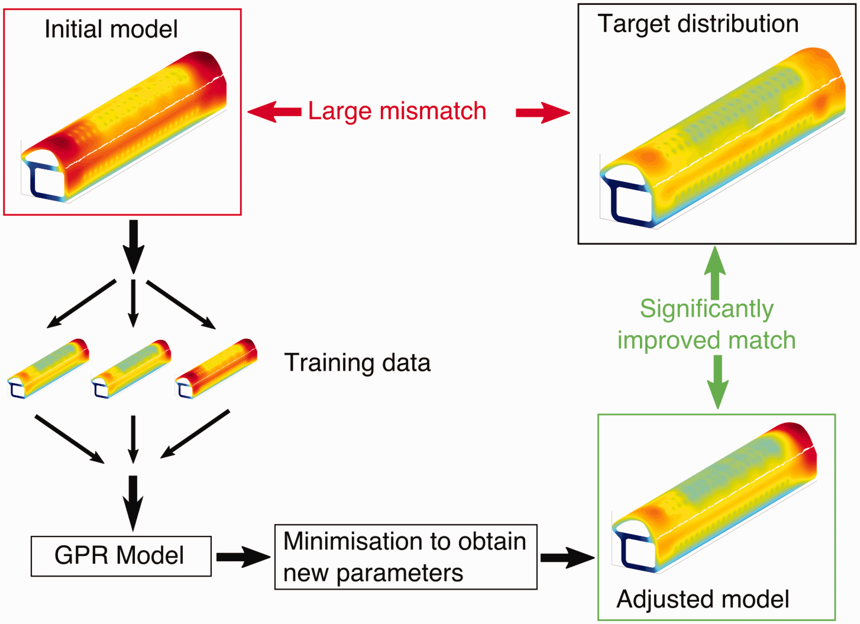
The new process by which the thermal matching is undertaken is illustrated in Figure 1, with the detailed procedure explained in the following section.

The required geometry is imported into a finite element analysis (FEA) thermal model, in this case an Ansys Workbench Steady-State Thermal model (www.ansys.com). Here it is meshed to a resolution fine enough for reasonable detail within the metal. The initial thermal boundary conditions are also defined at this stage.

Simulations are then run at multiple parameter points in order to obtain the training data for the model. The parameters used for the thermal matching will usually be factors by which the HTCs on various surfaces are multiplied. The training simulations run depend on the method of fitting to be used and must be carefully chosen in order to provide data of sufficient quality to the model.

The training data, consisting of the full metal temperature distribution and the HTC multipliers, is then exported into Matlab (uk.mathworks.com) for the model fitting.

A model is then created to represent the temperature–HTC relationship using the training data. Multiple methods can be used for this step, with the GPR method selected in this case described in further detail below.

A target temperature distribution, which in the case of gas turbine components corresponds to the thermal paint data, is then imported into Matlab in order for the initial model to be fitted.

New multipliers are then predicted from the model to fit the target distribution. This is obtained using an optimisation function with the target of minimising the mean square temperature difference.

New HTC distributions are then calculated from the predicted HTC factors and imported into the FEA solver.

The thermal model is then run with the new HTC levels in order to obtain the adjusted temperature distribution.

Finally, the temperature distribution calculated from the adjusted HTC levels is compared with the target distribution in order to check that a satisfactory match has been obtained.

Figure 1.

Schematic illustration of new thermal matching procedure.

Gaussian process regression

GPR is widely used in other engineering and scientific fields, where sometimes it is know as kriging, particularly in cases with a low number of parameters. Initially, the technique was developed in geostatics to interpolate spatially between a sparse number of two-dimensional data points. ² It is now widely used in the geological and meteorological fields for two- and three-dimensional spatial mapping.^3,4 More recently the method and those similar to it have been in the statistics and machine learning communities for higher order problems. The closest usages found in the literature to that applied in this paper were in an inverse heat conduction problem and in stress analysis where the finite element simulations to produce the stress distributions can be time consuming.^5,6 The paper extends the usage of the method considerably in many aspects. These include the use in a thermal simulation and matching problem and the combination of using multiple GPR models at different spatial locations with thermal parameters driving the model.

GPR models are probabilistic models that use training data in order to give predictions for a new input. This process involves modelling the outputs, y, as a function of the input parameters, x, in the form given by equation (1), where h(x) and β comprise a set of basis functions, and f(x) is a Gaussian process (GP) with zero mean and covariance function $k(x,x\text{'})$

$$y=h(x)T\beta +f(x)f(x)\sim \mathit{GP}(0,k(x,x\text{'}))$$

(1)

The basis function is an explicit function of the parameters at a given point, and is usually a simple polynomial, while the covariance function gives the relationship between the required parameter point and the training data points away from the basis function. The covariance function has zero mean and varies around the basis function value obtained from the parameters. The model must be fitted to the data in order to determine the model parameters. These are the basis function coefficients, covariance function coefficients and the noise level in the data.

The covariance function can be of many forms, such as the squared exponential form given in equation (2). It must be smooth, where a similar response is predicted given two close input and training parameter points. The length scale parameter within the covariance function may be the same for all predictors, or different, with values predicted from the training data. For the squared exponential covariance function that is used in this paper, σ_f defines the peak value, whilst σ_l determines the rate of decay away from the peak

$$k(x_i,x_j|\theta )={\sigma }_f^2\text{exp}[-\frac{1}{2}\frac{(x_i-x_j{)}^T(x_i-x_j)}{{\sigma }_l^2}]$$

(2)

After the model parameters have been fitted, the model can be used to predict a response given a new parameter point using equation (3), which gives how an instance of the response y can be modelled

$$P(y_i|f(x_i),(x_i))\sim N(y_i|h(x_i{)}^T\beta +f(x_i),{\sigma }^2)$$

(3)

The prediction at any given point is represented by a normal distribution with estimated noise variance, ${\sigma }^2$ . The mean is given by the sum of the basis function and the GP f(x) evaluated at a specific parameter point. Full details of GPR modelling can be found in Rasmussen, ⁷ and for the specific implementation used in this paper from Matlab. ⁸

In order to create the model, the training data must be obtained. This is done by running multiple simulations using different values of the input parameters and storing the output. In this case, the training data are the values of temperature evaluated for the thermal model with specific values of the HTC multiplication factors. In the equivalent of a one-dimensional model, this would correspond to the temperature at one location. More generally, the temperature is evaluated at multiple points. The training data points are obtained using a central composite design to define the HTC multiplication factors for each training simulation, which results in 15 training points for the three parameter case presented in this paper.

The GPR methodology is implemented in Matlab using new functions that are packaged within the statistics and machine learning toolbox. ⁸

Initially, a model is created using the training data. The fitrgp function from the toolbox uses the input parameter and response training data, and returns a RegressionGP model. This model contains the estimated basis function coefficients, noise variance and kernel parameters which have been fitted using a maximum marginal log likelihood method.^7,8 Within fitgrp , the basis function and kernel, or covariance, functions can also be specified along with initial fitting parameters.

The RegressionGP model can then be used to predict a response given new inputs (values of x) using the predict function. This function simply returns the predicted response, in this case temperature from the new HTC multipliers, and can also report estimates of the confidence intervals for the response.

The fmincon function finds the minimum value of a constrained, multi-variable non-linear function and is used to find the optimum HTC multipliers in order to fit the target data.

In the case of thermal matching, the above functions are applied on a node-by-node basis. The temperature data and HTC multipliers are used to create a model for each node individually. The multiple node, and therefore GP model, approach is used in order to obtain a good model of the physics of the underlying problem where different areas of the model can exhibit very different relationships to the input parameters. The individual temperature predictions from each model can also be compared to the nodal temperature distribution they are modelling, providing an intermediate validation step of the GP models. The fmincon function is then used to find the HTCs which minimize the mean-squared-difference between the target and predicted temperature, obtained using the predict function. Minimum and maximum individual and combined constraints are used within the fitting process in order to guarantee a predicted adjustment that is reasonably close to the original model and physically realistic. This also ensures the prediction remains within, or close to, the training data range which reduces modelling errors.

For a large finite element model mesh size, the minimisation can be applied on a subset of nodes in order to improve solution time. These nodes can be selected randomly, but ideally should have reasonably even spacing to most accurately represent the overall model.

Method validation

Before a thermal match was attempted against a realistic target temperature, a validation stage was undertaken. This was done on an LE impingement cooling system representative of one that might be found in an HP gas turbine blade. In this validation, the method was tested to match a target distribution obtained from known HTC adjustments. This allowed for both the match of the applied factors and resulting temperature distribution to be assessed. The GPR method only used the target temperature, and not the HTC adjustments, to give a realistic assessment of the method.

The GPR modelling requires a choice of both the number of target temperature nodes, and therefore GPR models, and covariance function. In this case, the squared exponential covariance function and 1000 nodes were used. This number of nodes was found to give a good balance between full representation of the physical features whilst not being too computationally expensive, whilst the squared exponential covariance function was used as it provided the most reliable modelling of the nodal temperatures.

Figure 2 shows the different regions where HTC adjustments were made. These are classified as the LE, web and coolant feed regions. The initial LE HTCs were taken from a conjugate computational fluid dynamics (CFD) solution, while those on other surfaces were calculated using the Dittus-Boelter correlation based on each individual passage Reynolds number. The upper and lower web surfaces therefore both have different initial HTC values, due to the different Reynolds number and passage dimensions, but in this case are subject to the same HTC adjustment factor. The Reynolds numbers based on the relevant hydraulic diameter for the feed, LE and impinging jet were 128,200, 49,300 and 54,500, respectively. The corresponding unadjusted Nusselt numbers are 245 for the feed and lower web, 114 for the upper web, with the conjugate CFD solution used for the LE having an average Nusselt number of 402.

Figure 2.

Leading edge impingement validation set-up.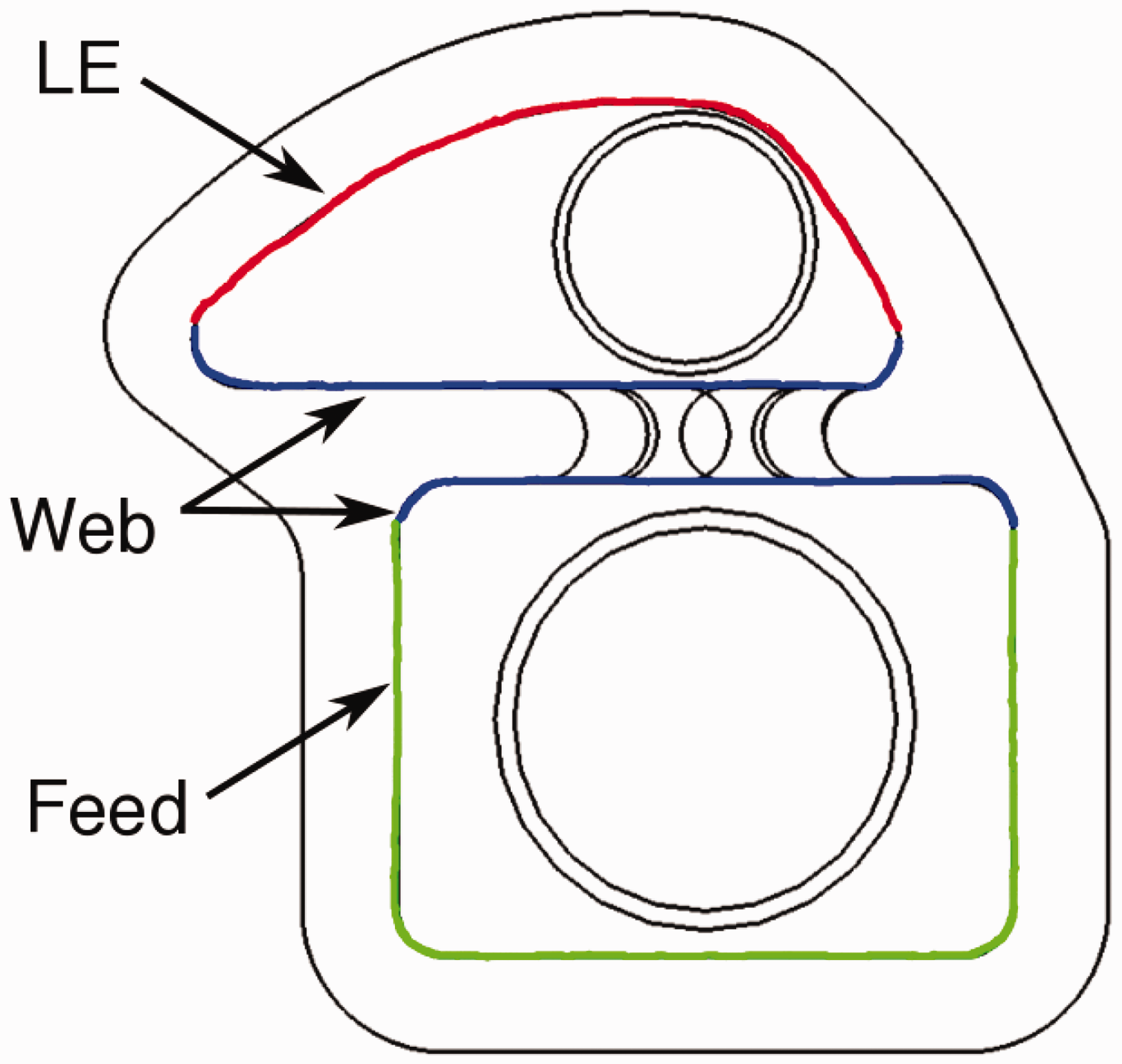

The target temperature distributions were generated with known HTC adjustments. These were an increase of each factor in turn, a common mode decrease and a common mode gain, which are given in Table 1.

Table 1.

HTC factors for validation.

Sim. No.	LE factor		Web factor		Feed factor
	Targ.	Adj.	Targ.	Adj.	Targ.	Adj.
1	1.25	1.237	1	0.998	1	0.999
2	1	1.00	1.25	1.228	1	1.000
3	1	1.00	1	0.997	1.25	1.234
4	0.75	0.759	0.75	0.769	0.75	0.762
5	1.25	1.239	1.25	1.227	1.25	1.235

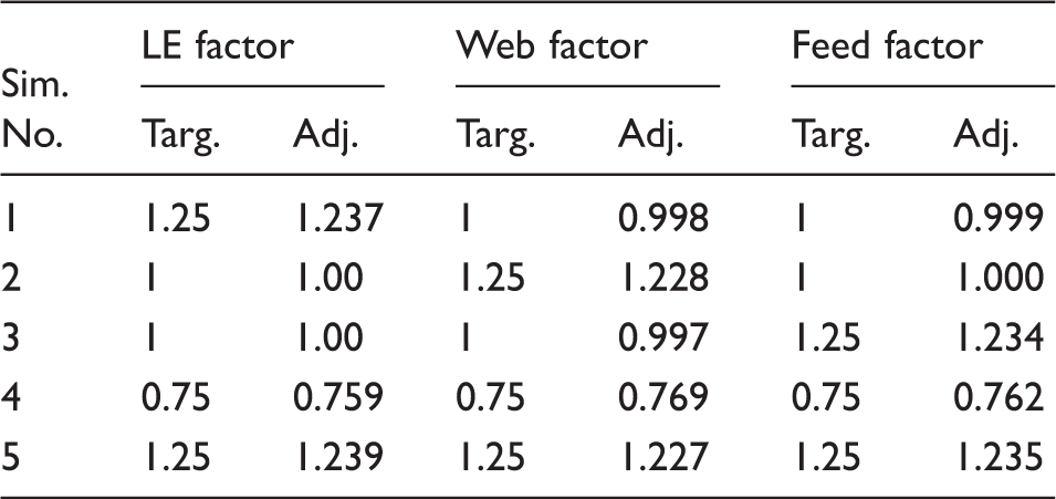
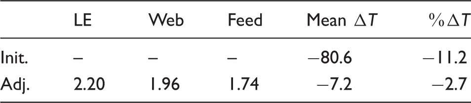
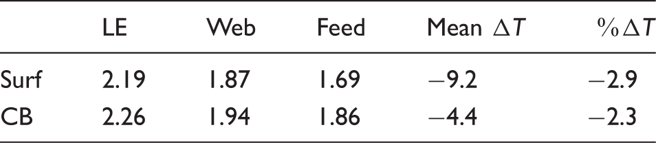
Table 1 gives the predicted HTC adjustments obtained using the GPR method compared with the target values. The predicted multipliers are very close (within 2%) to their targets with a consistent small underprediction in the change from the initial values. Therefore, in terms of HTC adjustments, this validation is very successful, and likely will also be in terms of the temperature distribution.

The mean temperature differences between the initial and adjusted, and target distributions for the validation simulations are given in Figure 3. It is clear that, as expected from the very good match of HTC factor levels, the adjusted temperature distribution is extremely close to the target distribution for all cases, despite a significantly different starting temperature difference. This indicates that this method should provide good quality, reliable predictions for LE impingement, and similar cooling systems.

Figure 3.

Leading edge validation – temperature results.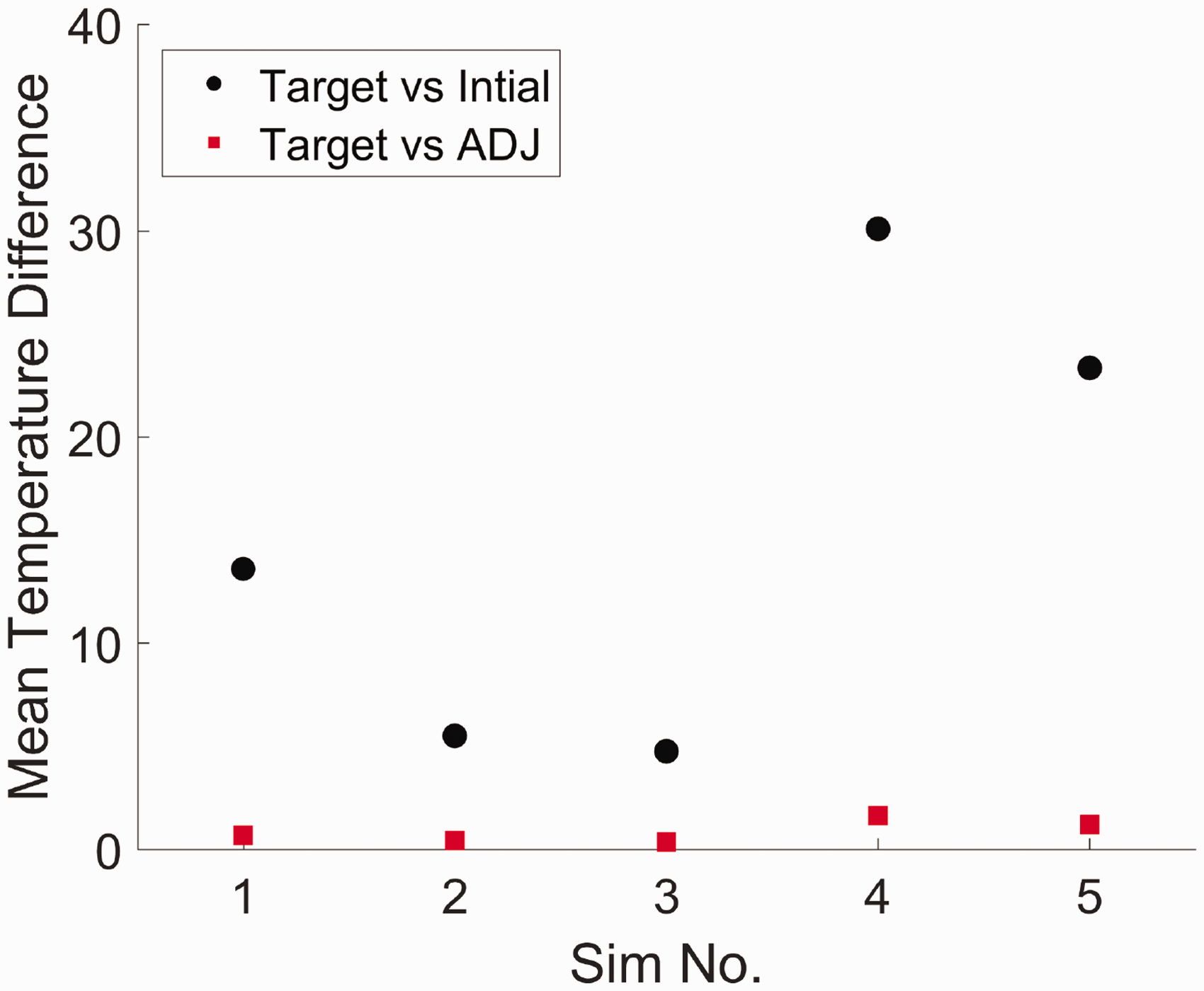

Following this validation, the GPR method using the set-up as detailed above was applied to a thermal matching that is very close to the ‘real’ situation to show its capability to undertake the temperature matching accurately, much faster and more consistently than the current manual methods.

Results and discussion

The matching method using GPR is now presented to perform a temperature matching for a situation very close to the thermal paint test, an LE impingement system, where it could ultimately be used most effectively.

The target distribution was set to be the full metal temperature distribution obtained from a conjugate CFD solution. The initial temperature distribution was obtained in a steady-state thermal FEA solution using HTC levels calculated from the passage Reynolds number and an LE internal HTC distribution from CFD. These are illustrated in Figure 4(a) and (b).

Figure 4.

Temperature distributions of full geometry for (a) target, (b) initial (c) and adjusted models.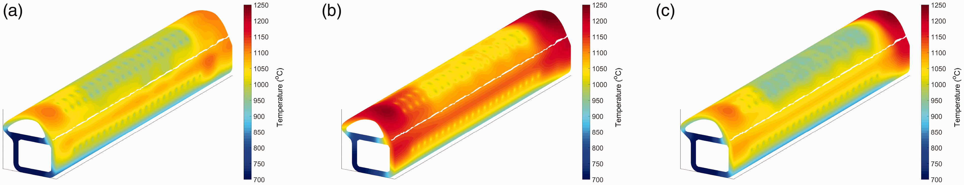

There is one adjusted model presented in this section, with HTC adjustment regions of the LE, web and feed as previously shown in Figure 2. An initial set-up that is not presented in this paper, but used adjustment regions on the LE, and upper and lower surfaces of the web could match the LE region well; however, the web and feed regions could not be matched as there was no adjustable factor local to this region. Therefore, the regions were changed leading to those presented here in order to address this.

The GPR method is able to choose the best factor to be applied to a datum solution, but the approach is dependent on the choice of sensible, physically reasonable, factors. The initial work before that presented here has shown that the aerothermal engineer using the method must exercise judgement as to which zones should be assigned independent factors.

The temperature distributions for the target, initial and adjusted simulations are shown in Figure 4. The adjusted simulation shows a significantly improved match over the initial distribution, which overestimates the temperature by a large amount in most regions. The adjusted simulations significantly increased the HTCs in all the adjustable regions.

The LE region is well matched by the adjusted simulation both in terms of the temperature levels and distribution, showing clearly the cooler metal at the location of the impingement jets as well as significantly higher temperatures in the uncooled areas. The matched model also obtains a close distribution across the web, feed and other sections of the geometry due to the increased HTCs in the feed region, enabling increased cooling of this section to more closely reflect the target distribution. The tip section of the blade is not well matched due to the absence of any adjustable HTC regions near to it. The match here that uses three parameters could be improved by using a larger number of adjustable parameters. However, increasing the number of parameters must be balanced against the increased computational cost that is introduced. Of course, as the computational power available to the aerothermal engineer increases with time, it will inevitably be possible to increase the number of factors used and therefore reduce the judgement required.

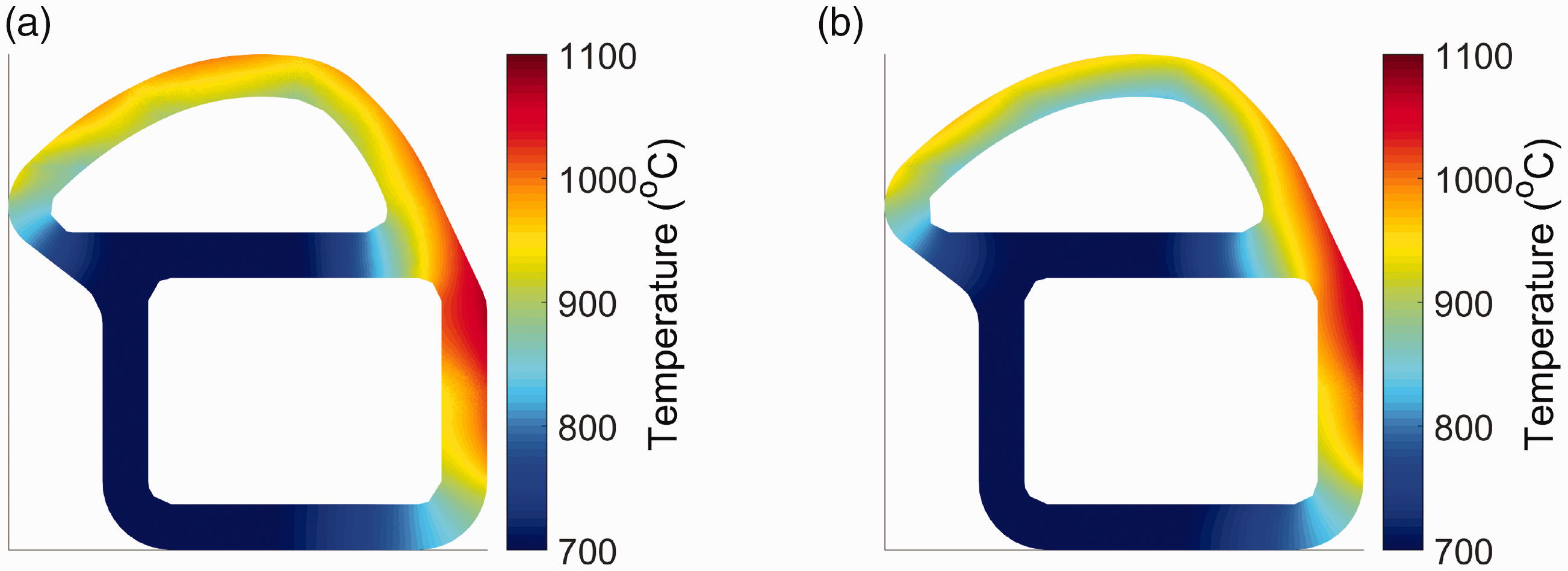
A mid-section slice of the temperature distribution discussed above is given in Figure 5, in order to compare the internal distribution in the most critical area of the matching process.

Figure 5.

Temperature distributions on mid-height cross-section for (a) target, (b) initial and (c) adjusted models.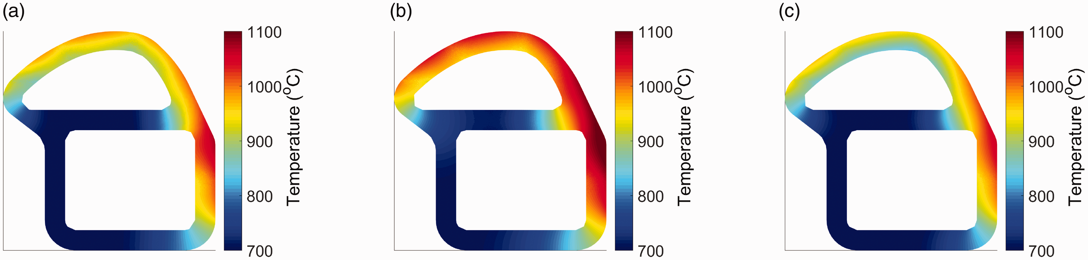

This comparison illustrates very clearly the improvements made to the match with the adjusted model. The initial distribution is very far from the target and therefore large HTC adjustments are required. The adjusted simulation, Figure 5(c), is a very close match to the target temperature. All the outer metal shells have a very similar temperature level and distribution with only a marginally lower peak value in the adjusted distribution on the outer edge near to the web. The web has a slightly different temperature distribution, however similar levels, due to a single HTC value being used across the web rather than a full distribution. A full distribution could be applied and then adjusted on these surfaces which would rectify this discrepancy.

Table 2 gives the numerical factors applied to the different regions for the adjusted model, and the mean and mean percentage nodal temperature differences between the target and modelled distributions. It is clear that the initial model is very far from the target, and with the applied HTC factors in the adjusted simulation, the match is significantly improved.

Table 2.

HTC adjustments and temperature comparison to target for initial and adjusted models.

	LE	Web	Feed	Mean $\Delta T$	$\%\Delta T$
Init.	–	–	–	−80.6	−11.2
Adj.	2.20	1.96	1.74	−7.2	−2.7

In general, the temperature matching using the GPR method is extremely successful, providing a very good temperature match in a standardised and much faster process.

Further results

In a real engine thermal paint test, a full three-dimensional target distribution is not available, only an outer surface temperature distribution is available. Therefore, the method must be validated with only surface target temperature used as an input.

Surface target distribution

The LE model and target distribution from the previous section will now be used to predict HTC adjustments where only the surface distribution is used for the target inputs.

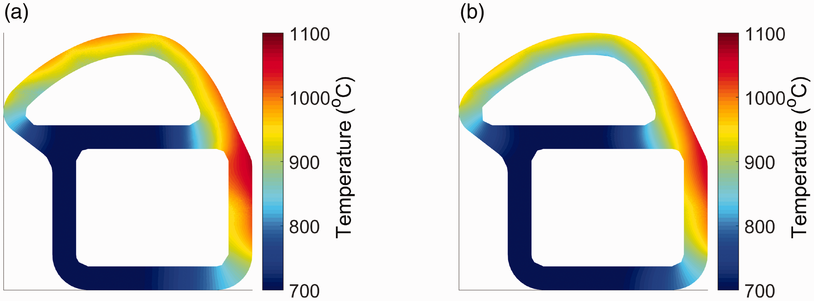
Figures 6 and 7 give the outer and mid-section metal temperature comparison between the target and adjusted distributions.

Figure 6.

Temperature distributions of full geometry for target and adjusted models with surface temperature input. (a) Target. (b) Adjusted.

Figure 7.

Temperature distributions on mid-height cross-section for target, initial and adjusted models with surface temperature input. (a) Target. (b) Adjusted.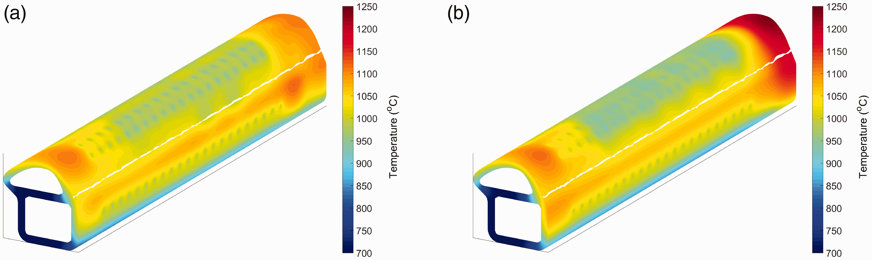

The temperature distribution is very well matched, as it was with the full three-dimensional target input, in both the surface and mid-chord slice. Both of these figures show clearly that the GPR-based prediction method works well with just a hot surface temperature distribution. This is also shown in Table 3, where the adjustment factors and temperature differences are very similar to those obtained when the full three-dimensional data are used as the target.

Table 3.

HTC adjustments and temperature comparison to target for surface and contour band models.

	LE	Web	Feed	Mean $\Delta T$	$\%\Delta T$
Surf	2.19	1.87	1.69	−9.2	−2.9
CB	2.26	1.94	1.86	−4.4	−2.3

Surface contours target distribution

The real thermal paint test does not produce a fully resolved surface temperature distribution but a series of contour bands at approximately 40 ℃ intervals. In order to simulate this, a number of temperatures spaced by 40 ℃ were chosen, and surface target points within 2 ℃ of them were selected and set to the central value of the contour band. All of the points selected are shown in Figure 8(a), with the nodes used for the HTC adjustment calculation given in (b), a subset of (a).

Figure 8.

(a) All node temperatures and (b) those selected for contour band input to model.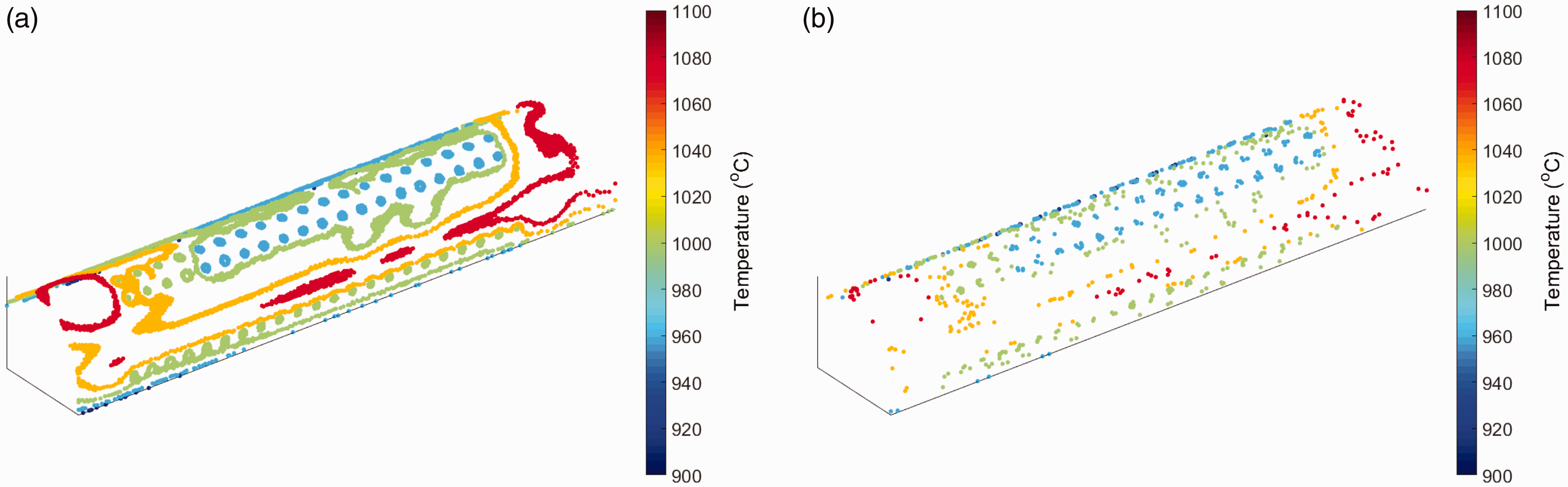

The resulting temperature distribution comparisons from using these contour band target inputs are given in Figures 9 and 10.

Figure 9.

Temperature distributions of full geometry for target, initial and adjusted models with contour band input. (a) Target. (b) Adjusted.

Figure 10.

Temperature distributions on mid-height cross-section for target, initial and adjusted models with contour band input. (a) Target. (b) Adjusted.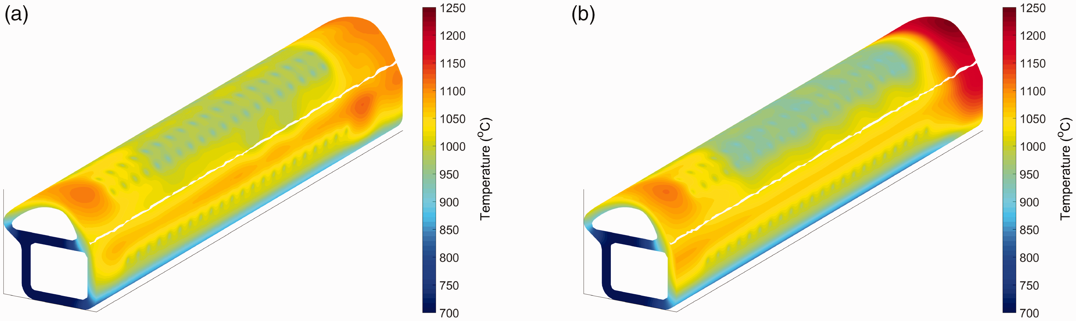

The use of these contour band inputs is clearly not problematic for this method as again a very good temperature match is obtained throughout the geometry, which is confirmed by the details give in Table 3 where the contour band input is seen to give the best match to the target distribution, the mean temperature being within 2% of the target.

It is clear from these results that the GP method presented in this paper is robust to the use of surface and contour band target distributions, which simulate the available data from a real engine thermal paint test most closely.

Summary and conclusions

The thermal matching process is a key stage in the engine design process; however, it is currently completed using a time-consuming, non-standardised procedure. A new method using GPR has been investigated. This method has been validated for a representative LE geometry with a very close match obtained between the adjusted and target distributions. The GPR model was then successfully applied to match to a full target distribution obtained from a conjugate CFD model. The following conclusions have been found:

The new method detailed and implemented in the paper has been demonstrated to offer reliable temperature matches using adjusted HTC values on selected internal surfaces.

The GPR-based method provides consistently good predictions for an LE geometry. It was then successfully applied to a realistic case similar to that required in a thermal paint match test.

The GPR method was proven to give very good thermal matches with full three-dimensional, surface and contour band inputs for this LE cooling configuration.

The new modelling and prediction method therefore offers a faster, more reliable alternative to the existing manual methods for thermal matching of gas turbine engine components.