Sage Journals: Discover world-class research

Abstract

Hyperspectral remote sensing technology becomes more and more popular in recent years which can be applied to satellite, plane, and flying robots. An important application of hyperspectral remote sensing is the classification of ground objects. However, when the number of labeled samples is very small, the classification accuracy of pixelwise classifiers will decline dramatically. In this article, a novel hyperspectral image classification approach is proposed based on multiresolution segmentation with a few labeled samples. The proposed method is motivated by the fact that pixels within a homogenous region are very likely to have the same class label, which can be utilized to increase the number of labeled samples. The proposed method consists of four steps. First, the hyperspectral image was segmented using the multiresolution image segmentation method. Second, the unlabeled neighbor pixels in the same region as the labeled pixels were selected randomly to assign the class labels. Next, one pixelwise classifier, that is, support vector machine, is used to classify the hyperspectral image with the new labeled sample set. Finally, edge-preserving filtering is performed on the classification result to remove the salt-and-pepper noise and preserve edges of ground objects. Experimental results on three real hyperspectral images demonstrate that the proposed method can improve the classification accuracy significantly when the number of labeled samples is relatively small.

Keywords

Principal component analysis segmentation edge-preserving filtering semi-supervised image classification support vector machine

Introduction

Hyperspectral remote sensing is a major breakthrough of remote sensing technologies. Hyperspectral sensors can be mounted on satellites or aircraft, including manned and unmanned aerial vehicles (UAVs). High spectral resolution images are available with hyperspectral sensors, such as the airborne visible/infrared imaging spectrometer (AVIRIS). Hyperspectral images provide detailed spectral information regarding the physical nature of the materials and thus can be used to distinguish different landscapes. Hyperspectral remote sensing images have been applied in many fields, such as environmental protection, precise agriculture, and so on.

However, the high dimensionality of hyperspectral data may produce the Hughes phenomenon¹ and have a bad impact on the performance of classification methods. Thus, it is necessary to reduce dimension of the hyperspectral image.² During the last decade, a large number of feature extraction³ techniques have been proposed to address the high-dimensionality problem, for example, principle component analysis (PCA),^4,5 decision boundary feature extraction,⁶ projection pursuit,⁷ and nonparametric weighted feature extraction.⁸ PCA as a data reduction dimension method has many advantages. For example, it is a simple algorithm and has no parameter restrictions. PCA can transform data into a lower dimensional feature space, so it can help to improve the classifier performance.

In order to solve the problem of insufficient or poor quality of the sample, people have studied various methods, such as robust sample selection,⁹ semi-supervised learning, and so on. Semi-supervised learning methods include the self-training,¹⁰ the transductive support vector machine (TSVM),¹¹ the generative model,^12,13 the graph-based methods,¹⁴ and so on. All of these methods can be used to predict the classes of unlabeled samples and improve the classification accuracy of hyperspectral images to a certain extent. There are some limitations for aforementioned methods when the number of labeled samples is relatively small, sometimes the classification results are completely wrong in the region without labeled samples. For example, self-training uses the previous classification results to train the classifier iteratively but it suffes largely from the incorrect labels.

To solve these problems, we present a simple and easy to implement method to generate new labeled samples. Image segmentation is used to generate new labeled sample for hyperspectral images classification. Image segmentation¹⁵ is the method of dividing the images into a number of specific regions with unique properties. At present, image segmentation has many different methods, for example, watershed, random walk-based image segmentation,¹⁶ graph-based image segmentation,¹⁷ region growing method,¹⁸ multiresolution segmentation method,¹⁹ and so on. Those image segmentation methods will generate a lot of homogeneous regions.²⁰ The pixels in the same region can be seen as belonging to the same classes. Based on this principle, the proposed method uses PCA to select the first principal component as the base image instead of the original hyperspectral image. The selected principal component is divided into a lot of regions by image segmentation method that is based on multiresolution segmentation. Several pixels were randomly selected and labeled in the region which contains the labeled samples which can generate new labeled samples. The purpose of random selection in the homogenous region is to make the selected unlabeled samples more representative.

The rest of this article is organized as follows. “Related techniques” section introduces three widely used techniques for hyperspectral image classification. “Proposed approach” section describes the proposed classification method. “Experiment results and discussions” section gives the results and provides a discussion. The final section draws the conclusion.

Related techniques

Principal component analysis

PCA tries to replace the original large number of correlation indicators and recombine into a new set of independent indicators. It can reduce the number of variables to a few comprehensive variables. Each principal component of the original variables is a linear combination, and the principal components are independent to each other. So the selected principal components can reflect the majority information of the initial variables. The process of the PCA is as follows.

First, construct a normalized matrix by normalizing the raw data

Z_{i j} = \frac{x_{i j} - {\bar{x}}_{j}}{s_{j}}

where i and j represent the ith and jth pixels, ${\bar{x}}_{j}$ represents the pixel mean, and s_j represents the image pixel standard deviation.

Second, the covariance matrix R is obtained from the normalized matrix

R = {[r_{i j}]}_{p} x p = \frac{Z^{T} Z}{n - 1}

with $r_{i j} = \frac{\sum z_{k} i \cdot z_{k j}}{n - 1} i, j = 1, 2, ... p$ .

The eigenvalues of covariance matrix are calculated and ranked in order of magnitude, that is, $λ_{1} \geq λ_{2} \geq, ... λ_{p} > 0$ . Then calculate the unit eigenvectors α_i according to λ_i.

The standardized indicator variables are converted into principal component F_i

F_{i} = α_{i} Z

Image segmentation–multiresolution segmentation

Image segmentation method²¹ aims at dividing an image into homogeneous regions. Multiresolution segmentation is a segmentation method based on region merging. The algorithm uses a bottom-up regional growth strategy. This method consists of the following steps:

1. The scale parameter T was defined as the decision termination condition.

2. Calculate spectral heterogeneity h _spectral

\begin{array}{l} h_{spectral} = \sum_{i = 1}^{n} ω_{i} σ_{i} \end{array}

where σ_i is the standard deviation of the i th band spectral values in the region, ω_i is the weight of the ith band, and n is the number of the band.

3. The shape heterogeneity h _shape is defined as follows

\begin{array}{l} h_{shape} = w_{u} u + (1 - w_{u}) v \\ u = \frac{E}{\sqrt{N}} \\ v = \frac{E}{Ł} \end{array}

where u and v are the smoothness and compactness of the region, respectively. w_u is the weight of smoothness, E is the actual boundary length of the region, N is the total number of pixels in the region, and L is the total length of the rectangular boundary in the region.

4. The regional heterogeneity is obtained by combining the spectral heterogeneity h _spectral with the shape heterogeneity h _shape

f = w_{s} h_{spectral} + (1 - w_{s}) h_{shape}

where w_s is the weight of spectrum.

5. The adjacent small regions are merged into larger regions by comparing the regional heterogeneity f with the predefined parameter T. If the two adjacent regions have the smallest heterogeneity, they will be merged.

Finally, when weighted heterogeneity in the merged region is greater than the predefined scale parameter, the merge process ends.

Bilateral filtering

Bilateral filtering^22,23 can preserve edge and remove the noise of images. The edge-preserving property of bilateral filtering is mainly achieved by combining the spatial domain function and the range kernel function in the convolution process. A typical kernel function is a Gaussian distribution function

\bar{f} (x) = η^{- 1} \int_{Ω} w_{σ_{s}^{}} (y) φ_{σ_{r}} (f (y) - f (x)) d y

with

η = \int_{Ω} w_{σ_{s}^{}} (y) φ_{σ_{r}} (f (y) - f (x)) d y

where σ_s is the standard deviation of the spatial Gaussian function, σ_r is the standard deviation of the range Gaussian function, and Ω denotes the domain of the convolution.

Proposed approach

As illustrated in Figure 1, the first principal component obtained through PCA transform of the hyperspectral image was segmented into many small regions. Unlabeled samples in the same region as labeled samples are selected randomly to assign them the class label, which increases the number of labeled samples. The initial probability that a pixel belongs to a specified class is estimated based on SVM classifier. The final probabilities are obtained by performing edge-preserving filtering on the classification maps, with the first principal component serving as the guidance image. The proposed classification method can effectively generate new labeled samples and improve the classification accuracy.

Figure 1.

Schematic of the proposed semi-supervised classification method.

The proposed approach consists of four steps: (1) PCA transform and segmentation of the hyperspectral image, (2) generation of the new labeled samples, (3) classification of hyperspectral image using SVM classifier, and (4) refinement of the classification map using edge-preserving filtering.

Step 1: Hyperspectral image segmentation. PCA transform is conducted first on the original hyperspectral image, and the first principal component was obtained which contains most of the image information. One popular image segmentation method, that is, multiresolution segmentation, is used to segment the first principal component, which is segmented into many small regions. Specifically, in our implementation, the scale is set to 10–100, and the proportion of color and shape weight is set to 0.5 and 0.1, respectively.

Step 2: Generation of the new labeled samples. After the image is segmented, those pixels in each region usually have similar characteristics according to the homogeneity criterion. Based on this, we can select some pixels from the unlabeled samples to assign them labels of their neighbor pixels in the same region.

For each sample (x_i , y_i ) in the labeled samples set D, we will generate some related labeled samples as follows:

Obtain the region number of the current sample x_i .

All unlabeled samples within the same region as the sample x_i are extracted from the hyperspectral image and arranged into a column vector V.

Randomly permute the column vector V and select the first several unlabeled samples to form a set Z. The samples in the set Z are labeled as y_i . This step is also called labeled samples generation process.

The new generated labeled samples set Z is added to the final labeled samples set S

S = S \cup Z

The above procedure will continue until all initial labeled samples have been processed.

Step 3: Classification of the hyperspectral image with the updated labeled sample set. An initial classification map C can be obtained by a pixelwise classifier. In this article, the pixelwise classification map C is represented using a group of probability maps, that is, P = (P ₁,…, P_n ), where n is the number of classes. Each probability map is a binary image. If the class label of one pixel x_i,j is equal to k in the initial classification map C, then the corresponding pixel is set to 1 in P_k and 0 in other probability maps. In other words, for each pixel of the hyperspectral image, only one probability map can have value 1 in its location.

The SVM classifier is adopted for pixelwise classification since it is one of the most widely used pixelwise classifiers and has been successfully used in other supervised or semi-supervised classification methods. The SVM algorithm is implemented in the LIBSVM library.

Step 4: Filtering of the probability maps. Initially, all probabilities are valued at either 0 or 1 in the probability maps. Therefore, it appears noisy and not aligned with real object boundaries. To solve this problem, the probability maps are optimized by bilateral filtering. Specifically, the optimized probabilities are modeled as a weighted average of its neighborhood probabilities

P_{i, k} = \sum_{j} w i, j (I) P j, k

where P_j,k represents the value of jth pixel in the probability map P_k , represents the value of the ith pixel in the optimized probability map P_k , w_i,j represents the weight of the jth neighborhood pixel, which is computed using spatial domain function and the range kernel function, and I represents the guidance image, which is the first principal component of the hyperspectral image.

According to equation (7), once the probability maps are filtered, the label at pixel i can be simply chosen in a maximization manner as follows

c i = arg \frac{max}{k} P_{i, k}

This step aims at transforming the probability maps P_i,k into the final classification result.

Experiment results and discussions

Experimental setup

Data setup

Three remote sensing hyperspectral data sets, that is, the Indian Pines image, the University of Pavia image, and the Salinas image, are utilized in our experiments.

The Indian Pines image was acquired by the AVIRIS sensor. It captures the agricultural Indian Pine unlabeled site of Northwest Indiana and contains 220 bands of 145 × 145. Twenty water absorption bands (nos. 104–108, 150–163, and 220) were removed before hyperspectral image classification. Furthermore, the spatial resolution of the Indian Pines image is 20-m per pixel, and the spectral coverage is ranging from 0.4 µm to 2.5 µm. Figure 2 shows the color composite of the Indian Pines image and the corresponding ground truth data.

Figure 2.

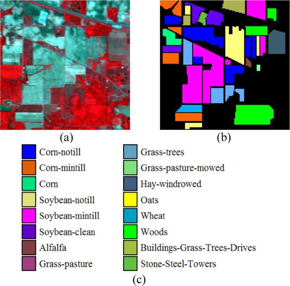
(a) Three-band color composite of the Indian Pines image. (b) and (c) Ground truth data of the Indian Pines images.

The University of Pavia image capturing the University of Pavia, Italy, was recorded by the reflective optics system imaging spectrometer. This image contains 115 bands of size 610 × 340 with a spatial resolution of 1.3-m per pixel and a spectral coverage ranging from 0.43 to 0.86. Before the classification, 12 noisy channels were removed, which is a standard preprocessing approach before hyperspectral image classification. Nine classes of interest are considered for this image. Figure 3 shows the color composite of the University of Pavia image and the corresponding ground truth data.

Figure 3.

(a) Three-band color composite of the University of Pavia image. (b) and (c) Ground truth data of the University of Pavia images.

The Salinas image was captured by the AVIRIS sensor over Salinas Valley, California, and it has a spatial resolution of 3.7-m per pixel. The Salinas image contains 224 bands of size 512 × 217, and 20 water absorption bands (nos. 108–112, 154–167, and 224) were discarded before classification. Figure 4 shows the color composite of the Salinas image and the corresponding ground truth data.

Figure 4.

(a) Three-band color composite of the Salina image. (b) and (c) Ground truth data of the Salina images.

Evaluation metrics

In order to evaluate the performance of image classification, three objective quality indexes, that is, the overall accuracy (OA), the average accuracy (AA), and the κ coefficient, are utilized for objective evaluation. Specifically, the OA index refers to the percentage of pixel that is correctly labeled in the classification. The AA index measures the mean of the percentage of correctly labeled pixels for each class. Finally, the κ coefficient calculates the percentage of correctly classified pixels.

Classification results

Analysis of the influence of parameters

For the proposed method, the number of generate new labeled samples in a region and the size of scale parameter in the multiresolution segmentation are influence to classification accuracies. The number of labeled samples and principal components obtained by the PCA and the size of the edge-preserving filtering window will affect the classification results by the proposed method in this article.

In the experiments, support vector machine(SVM), principal component analysis(PCA), image fusion and recursive filtering (IFRF), label propagation (LP) of based on semi-supervised are processed the original data. The proposed method PCA transform, Segmentation and Edge-Preserving Filtering (PSEPF) selects the first principal component and generates 10 labeled samples in a region. Multiresolution segmentation method is used to segment the first principal component. The guide image of EPF is a classification result generated by SVM, and the bilateral filtering is adopted. The size of region is 100 pixels.

In order to reduce the influence of the randomness of labeled samples, the experiment was repeated 30 times. The average of the 30 times experimental results as the final classification result.

Comparison of different classification methods

In this section, the proposed methods (PSEPF) are compared with the SVM, PCA, EPF, LP, and IFRF methods.

The first and second experiments are performed on the Indian Pines data sets. Figure 5 shows the classification maps obtained by different methods associated with the corresponding OA scores. From this figure, it can be seen that the classification accuracy obtained by the SVM and EPF methods is not very satisfactory since some noisy estimations are still visible. By contrast, the IFRF method and the proposed method perform much better in removing “noisy pixels.” Specifically, the proposed method increases the OA compared to the SVM method by about 30%. Compared with the recently proposed classification method (IFRF), the proposed method also gives a higher classification accuracy.

Figure 5.

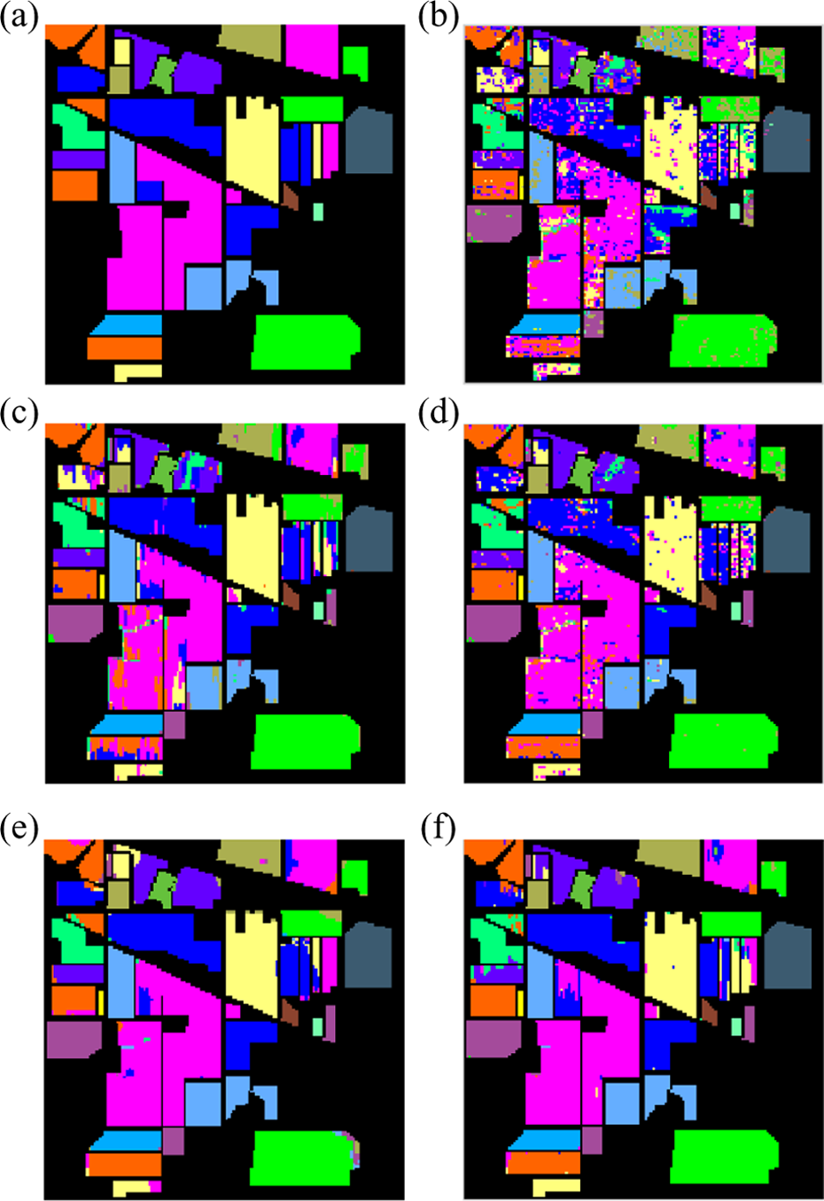
Classification results (Indian Pines image) obtained by the (a) reference land-cover, (b) SVM method (OA=73.1), (c) EPF method (OA=82.15), (d) LP method (OA=88.42), (e) IFRF method (OA=93.10), and (f) the proposed method (OA=95.17). The value of OA is given in percentage. The number of labeled samples is 5%. SVM: support vector machine; LP: label propagation; IFRF: image fusion and recursive filtering; OA: overall accuracy.

Table 1 presents the number of labeled and unlabeled samples (the labeled set which accounts for 2.5% of the ground truth was chosen randomly) and the classification accuracies for different methods. From this table, it can be observed that, using the proposed PSEPF method, the AA of SVM is increased from 63% to 90% and the κ accuracy can also be increased significantly. The proposed PSEPF method gives the best performance in terms of OA, AA, and κ. Table 2 presents the number of labeled and unlabeled samples (the labeled set which accounts for 5% of the ground truth was chosen randomly) and the classification accuracies for different methods. From this table, it can be seen that classification accuracy is significantly improved. In short, SVM method accuracies are less than 80%, and other methods are more than 80%, while accuracy of the proposed method and the method IFRF is more than 90%. At present, the supervised classification method has met the bottleneck of accuracy improvement.

Table 1.

Classification accuracy (in percentage) of different classification methods (the labeled set which accounts for 2.5%).

Class	Labeled	Unlabeled	SVM	EPF	LP	IFRF	PSEPF
Alfalfa	16	30	32.1	61.7	68.83	96.8	100
Corn_N	16	1412	59.5	78.1	80.05	93.4	85.7
Corn_M	16	814	34.8	39.5	65.77	73.8	82.5
Corn	16	221	31.6	35.6	69.6	86.6	67.6
Grass_M	18	465	67.4	80.6	93.57	72.1	87.9
Grass_T	16	714	88.7	93	96.42	99.1	97
Grass_P	14	14	85.7	100	84.09	30.4	100
Hay_W	17	461	97.6	99.3	99.04	100	100
Oats	10	10	26.3	45.5	79.44	90.9	76.9
Soybean_N	17	955	55	65.3	70.48	83.2	84.8
Soybean_M	18	2437	77.4	86.1	84.58	90.7	97.6
Soybean_C	16	577	33.2	38.3	71.35	87.3	82.7
Wheat	16	189	92.6	100	99.51	95.9	100
Woods	16	1249	91	93.5	98.02	95.9	99.3
Buildings	16	370	54.6	76	58.69	86.7	92.8
Stone	18	75	82.8	89	72.57	98.7	91.7
OA	—	—	63.35	73.32	80.91	88.89	90.88
AA	—	—	63.16	73.84	80.75	86.35	90.4
κ	—	—	58.92	62.17	78.51	68.89	87.37

SVM: support vector machine; LP: label propagation; IFRF: image fusion and recursive filtering; OA: overall accuracy; AA: average accuracy. The signification of the italic value is the method has the highest classification accuracy for a certain feature.

Table 2.

Classification accuracy (in percentage) of different classification methods (the labeled set which accounts for 5%).

Class	Labeled	Unlabeled	SVM	EPF	LP	IFRF	PSEPF
Alfalfa	23	23	73.91	91.3	86.91	95.65	100
Corn_N	42	1386	67.68	85.42	84.575	89.65	93.12
Corn_M	34	796	69.29	82.52	82.985	88.04	94.96
Corn	33	204	37.06	42.71	67.89	88.11	67.01
Grass_M	34	449	89.88	97.8	95.56	97.07	95.73
Grass_T	38	692	93.51	98.5	98.53	97.88	99
Grass_P	14	14	81.25	93.33	98.215	82.35	100
Hay_W	35	443	98.42	99.78	99.375	100	100
Oats	10	10	45	71.43	95.455	90.91	90.91
Soybean_N	38	934	60.19	66.04	77.855	83.93	90.29
Soybean_M	44	2411	79.4	87.83	90.815	97.23	98.58
Soybean_C	33	560	58.87	73.42	80.07	83.75	88.58
Wheat	33	172	88.3	97.16	99.755	99.42	100
Woods	36	1229	95.67	97.82	97.305	100	99.92
Buildings	32	354	41.98	55.1	77.095	90.18	96.41
Stone	33	60	87.69	88.06	92.16	98.36	93.75
OA	—	—	73.10	82.15	87.96	93.10	95.17
AA	—	—	73.01	83.01	89.035	92.66	94.27
κ	—	—	69.53	79.75	86.365	92.13	94.48

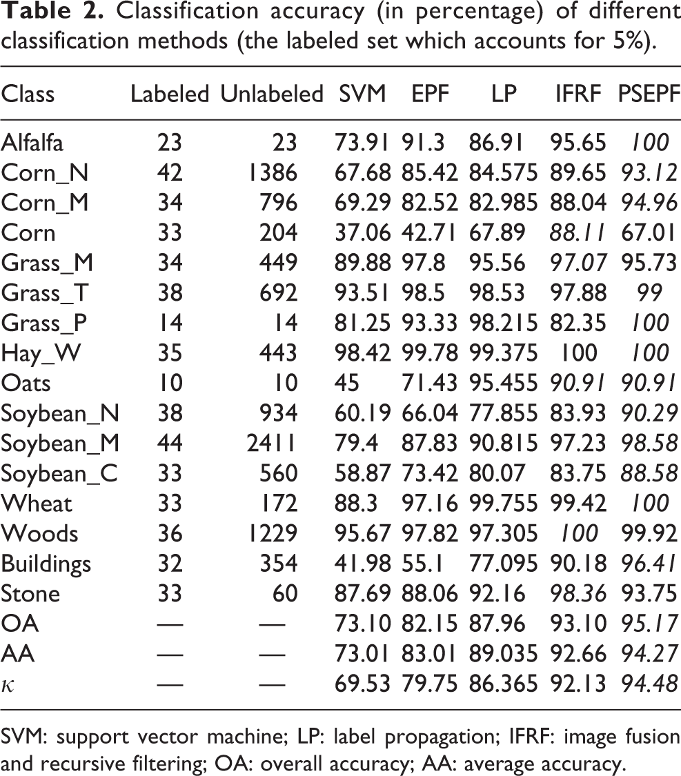
SVM: support vector machine; LP: label propagation; IFRF: image fusion and recursive filtering; OA: overall accuracy; AA: average accuracy.

The second and third experiments were performed on the University of Pavia image. Figures 6 and 7 show the classification maps obtained by different methods associated with the corresponding OA scores. Tables 3 and 4 present the number of labeled and unlabeled samples (for the University of Pavia image, the labeled sets which, respectively, account for 0.3 and 2% of the ground truth were chosen randomly) and the classification accuracies for different methods.

Figure 6.

Classification results (University of Pavia image) obtained by the (a) reference land-cover, (b) SVM method (OA=69.46), (c) EPF method (OA=74.42), (d) LP method (OA=80.52), (e) IFRF method (OA=82.73), and (f) the proposed method (OA=93.32). The value of OA is given in percentage. The number of labeled samples is 0.3%. SVM: support vector machine; LP: label propagation; IFRF: image fusion and recursive filtering; OA: overall accuracy.

Figure 7.

Classification results (University of Pavia image) obtained by the (a) reference land-cover, (b) SVM method (OA=87.40), (c) EPF method (OA=93.52), (d) LP method (OA=92.28), (e) IFRF method (OA=96.43), and (f) the proposed method (OA=98.51). The value of OA is given in percentage. The number of labeled samples is 2%. SVM: support vector machine; LP: label propagation; IFRF: image fusion and recursive filtering; OA: overall accuracy.

Table 3.

Classification accuracy (in percentage) of different classification methods (the labeled set which accounts for 0.3%).

Class	Labeled	Unlabeled	SVM	EPF	LP	IFRF	PSPEF
Asphalt	15	6616	97.84	98.65	97.78	82.7	99.41
Meadows	15	18,634	89.08	90.8	96.82	97.48	98.59
Gravel	14	2085	51.86	65.87	73.54	75.5	95.53
Trees	14	3050	48.11	48.3	63.24	43.86	81.15
Sheets	14	1331	94.42	94.38	98.88	100	93.38
Soil	14	5015	58.83	73.39	66.28	84.34	81.6
Bitumen	14	1316	47.79	58.5	53.32	70.08	80.9
Bricks	14	3668	76.03	80.8	80.5	79.74	88.81
Shadows	14	933	100	99.25	94.96	48.28	99.57
OA			69.21	73.76	80.06	82.10	90.55
AA			71.21	76.24	80.59	76.10	88.88
κ			61.63	67.16	78.48	76.94	87.81

SVM: support vector machine; LP: label propagation; IFRF: image fusion and recursive filtering; OA: overall accuracy; AA: average accuracy.

Table 4.

Classification accuracy (in percentage) of different classification methods (the labeled set which accounts for 2%).

Class	Labeled	Unlabeled	SVM	EPF	LP	IFRF	PSPEF
Asphalt	95	6536	98.52	99.33	97.12	93.81	99.57
Meadows	95	18,554	96.73	98.88	98.74	99.65	99.73
Gravel	95	2004	68.61	82.80	82.59	93.40	97.09
Trees	95	2969	76.26	83.68	91.91	93.36	96.02
Sheets	95	1250	98.89	99.52	99.76	100	99.92
Soil	95	4934	70.77	82.22	79.37	95.71	98.56
Bitumen	95	1235	60.56	78.54	78.27	93.48	97.07
Bricks	95	3587	83.93	89.20	89.67	87.77	94.12
Shadows	95	852	99.88	99.07	91.74	87.87	97.15
OA			87.40	93.52	92.65	96.43	98.54
AA			84.48	91.62	89.91	94.01	97.89
κ			83.57	91.47	90.41	95.26	98.05

SVM: support vector machine; LP: label propagation; IFRF: image fusion and recursive filtering; OA: overall accuracy; AA: average accuracy.

Figure 6 shows the classification maps obtained by the labeled set which accounts for 0.3% of the ground truth. Figure 7 shows the classification maps obtained by the labeled set which accounts for 2% of the ground truth. The proposed method has the better classification accuracies of OA.

From Figures 6 and 7, it can be seen that the classification accuracies obtained by the proposed methods are always the highest. It is observed that SVM and EPF method accuracies are less than 80%, and other methods are more than 80% when the number of labeled samples is 0.3%. By contrast, when the number of labeled samples is 2%, the OA of all of the method increase widely, especially, the proposed method is up to 98%.

Table 3 presents the number of labeled and unlabeled samples (the labeled set which accounts for 0.3% of the ground truth was chosen randomly) and the classification accuracies for different methods. From this table, it can be seen that the proposed method always outperforms the SVM, EPF, LP, and IFRF. In addition to the classification accuracies of the sheets and soil class less than IFRF, other classification accuracies of other class are better than the other method.

Table 4 presents the number of labeled and unlabeled samples (the labeled set which accounts for 2% of the ground truth was chosen randomly) and the classification accuracies for different methods. From this table, it can be seen that the classification accuracy of every classification method is improved. Especially, the classification accuracy of SVM, EPF, and LP is improved drastically.

The fifth experiment is performed on the Salinas image data sets. Table 5 presents the number of labeled and unlabeled samples (the labeled set which accounts for 0.1% of the ground truth was chosen randomly) and the classification accuracies for different methods. From Table 5, it can be found that the proposed method is generally higher than SVM, EPF, LP, and IFRF methods. When the number of labeled sample is 0.1% of the reference data, the proposed method percentage of the classification average accuracies is up to 94%.

Table 5.

Classification accuracy (in percentage) of different classification methods (the labeled set which accounts for 0.1%).

Class	Labeled	Unlabeled	SVM	EPF	LP	IFRF	PSEPF
Weeds_1	3	2006	96.68	99.50	99.87	100	100
Weeds_2	3	3723	99.34	99.86	99.03	100	99.52
Fallow	3	1973	100	0	83.16	99.80	92.40
Fallow_p	3	1391	97.62	98.10	97.17	76.85	95
Fallow_s	3	2675	74.31	74.16	99.27	99.96	99.42
Stubble	3	3956	99.39	100	94.27	100	100
Celery	4	3575	96.60	96.57	91.67	96.12	97.72
Grapes	6	11,265	58.81	58.57	64.5	89.08	88.47
Soil	3	6200	99.23	99.55	98.87	99.94	99.37
Corn	3	3275	76.89	83.56	81.7	99.96	97.91
Lettuce_4	4	1064	96.41	98.94	89.08	97.72	86.19
Lettuce_5	4	1923	75.22	75.33	95.59	93.97	96.10
Lettuce_6	3	913	96.94	99.78	92.35	85.49	99.22
Lettuce_7	3	1067	0	0	90.34	46.27	66.92
Vinyard_U	3	7265	21.08	3.25	48.49	89.34	96.90
Vinyard_T	3	1804	9.84	6.84	92.48	100	99.65
OA			70.40	72.00	80.96	83.57	93.02
AA			77.21	78.81	88.62	84.49	94.18
κ			67.18	68.92	78.85	81.73	92.23

SVM: support vector machine; LP: label propagation; IFRF: image fusion and recursive filtering; OA: overall accuracy; AA: average accuracy.

Figure 8 shows the classification maps obtained by different methods of the Salinas image associated with the corresponding OA value. Compared with the SVM method, the proposed method can improve the classification accuracies significantly. For example, in Figure 8, the classification accuracy of the proposed method is 93.02%.

Figure 8.

Classification results (Salinas image) obtained by the (a) reference land-cover, (b) SVM method (OA=70.40), (c) EPF method (OA=72.0), (d) LP method (OA=80.88), (e) IFRF method (OA=83.57), and (f) the proposed method (OA=93.02). The value of OA is given in percentage. The number of labeled samples is 0.1%. SVM: support vector machine; LP: label propagation; IFRF: image fusion and recursive filtering; OA: overall accuracy.

From those experiments, the proposed method has attained the highest value in κ, OA, and AA. It can be seen that this method is not only excellent in the case of a few labeled samples but also has some advantages when the number of samples is adequate.

Classification results with different labeled and unlabeled samples set

In this section, the influence of different labeled and unlabeled sets to the performance of the proposed method is analyzed. Experiments are performed on three images, that is, the Indian Pines image, the University of Pavia image, and the Salinas image. The classification result obtained by the proposed method is presented. Figure 9 shows the classification results of the proposed method with the number of labeled samples (in percent) increased from 0.0625% to 5% for the Indian Pines image, 0.1% to 0.5% for the University of Pavia image, and 0.05% to 0.25% for the Salinas image.

Figure 9.

Classification accuracy of the different hyperspectral image.

From this figure, it can be seen that the proposed method can always improve the classification accuracy significantly with a different number of labeled samples. For example, regarding the Indian Pines image, when the OA of SVM is about 70% (3.75% ground truth samples are used as labeled samples), the proposed method can obtain a classification accuracy near 94%. For the University of Pavia image, it can be seen that, with relatively limited labeled samples (0.5% of the ground truth), the proposed method can obtain an OA up to 95%. A similar conclusion can be obtained when analyzing the experimental results of the Salinas image, when relatively limited labeled samples (0.05% of the ground truth), the proposed method can obtain a classification accuracy near 84% and other methods have lower than the proposed method; the classification accuracy of IFRF method is only 31%.

The experimental results show that the proposed method shows very good classification performances for three widely used real hyperspectral data sets even when the number of training samples is extremely small. Meanwhile, there is a need to pay for more cost of computational complexity when the number of samples is very large.

Conclusion

This article presents a semi-supervised segment-based hyperspectral image classification method with a few labeled samples. The key idea of the article is that the pixels within the same region are homogenous, so they should have similar labels. Those new labeled samples are generated by label of the unlabeled samples in the segmented region. The major advantage of the proposed method is that it is able to increase the number of labeled samples for label of SVM classifier. Experimental results demonstrate that the proposed method achieves higher classification accuracy than other out-of-date methods.

The contribution of this article is that it proposed a new, simple, and effective method to improve the classification accuracy by increasing the number of training samples. This method solves the problem of low classification accuracy which is caused by the insufficient sample.

Footnotes

Declaration of conflicting interests

The author(s) declared no potential conflicts of interest with respect to the research, authorship, and/or publication of this article.

Funding

The author(s) disclosed receipt of the following financial support for the research, authorship, and/or publication of this article: This work was co-supported by the National Natural Science Foundation of China (41406200) and Shandong Province Natural Science Foundation of China (ZR2014DQ030).

References

Hughes

. On the mean accuracy of statistical pattern recognizers. IEEE Trans Inf Theory 1968; 14(1): 55–63.

Zhang

Zhong

Huang

. Dimensionality reduction based on clonal selection for hyperspectral imagery. IEEE Trans Geosci Remote Sens 2007; 45(12): 4172–4186.

Nixon

Aguado

AS.

Appendices - Feature Extraction and Image Processing - 9[J]. Feature Extraction Image Processing 2002; 138(2–4): 311–343.

Deutsch

. Principle component analysis. UK: Palgrave Macmillan, 2004.

Prasad

Bruce

. Limitations of principal components analysis for hyperspectral target recognition. IEEE Geosci Remote Sens Lett 2008; 5(4): 625–629.

Lee

Landgrebe

. Feature extraction based on decision boundaries. IEEE Trans Pattern Anal Mach Intell 1993; 15(4): 388–400.

Sun

. Projection Pursuit. Encyclopedia of Biostatistics. John Wiley & Sons, Ltd, 2005: 208–215.

Kuo

Landgrebe

. Nonparametric weighted feature extraction for classification. In: Ai 2005: advances in artificial intelligence, Australian joint conference on artificial intelligence, Sydney, Australia, 5–9 December 2005.

Liu

Sun

. Robust exemplar extraction using structured sparse coding. IEEE Trans Neural Network Learn Syst 2015; 26(8): 1816–1821.

10.

Rosenberg

Hebert

Schneiderman

. Semi-supervised self-training of object detection models. In: Workshop on applications of computer vision, IEEE Computer Society, 2005: 29–36.

11.

Gammerman

. Transductive learning. Pittsburgh: Springer, 2011. p. 990.

12.

Sabuncu

Yeo

BTT

Van Leemput

. A generative model for image segmentation based on label fusion. IEEE Trans Med Imaging 2010; 29(10): 1714–1729.

13.

Goodman

Mansinghka

Roy

. Church: A language for generative models. In: UAI 2008, proceedings of the conference in uncertainty in artificial intelligence. Helsinki, Finland, July 2008, pp. 220–229. DBLP.

14.

Aittokallio

Schwikowski

. Graph-based methods for analysing networks in cell biology. Brief Bioinformat 2006; 7(3): 243–255.

15.

Shi

Malik

. Normalized cuts and image segmentation. IEEE Trans Pattern Anal Mach Intell 2000; 22(8): 888–905.

16.

Grady

. Random walks for image segmentation. IEEE Trans Pattern Anal Mach Intell 2006; 28(11): 1768–1783.

17.

Felzenszwalb

Huttenlocher

. Efficient graph-based image segmentation. Int J Comput Vision 2004; 59(2): 167–181.

18.

Adams

Bischof

. Seeded region growing. IEEE Trans Pattern Anal Mach Intell 1994; 16(6): 641–647.

19.

Petrovic

Escoda

Vandergheynst

. Multiresolution segmentation of natural images: from linear to nonlinear scale-space representations. IEEE Trans Image Proc 2004; 13(8): 1104–1114.

20.

Mukawa

Uchiyama

Kaneko

. Estimation of homogeneous regions for segmentation of textured images. International Conference on Pattern Recognition, IEEE Computer Society, 2000: 7084.

21.

Jiang

Zhang

. A robust audio classification and segmentation method. In: ACM International Conference on Multimedia, ACM, 2001: 203–211.

22.

Tomasi

Manduchi

. Bilateral filtering for gray and color images: Proceedings of the 1998 IEEE international conference on computer vision, Bombay, India, 1998: 839.

23.

Kang

Benediktsson

. Spectral–spatial hyperspectral image classification with edge-preserving filtering. IEEE Trans Geosci Remote Sens 2014; 52(5): 2666–2677.

A novel hyperspectral image classification approach based on multiresolution segmentation with a few labeled samples

Abstract

Keywords

Introduction

Related techniques

Principal component analysis

Image segmentation–multiresolution segmentation

Bilateral filtering

Proposed approach

Experiment results and discussions

Experimental setup

Data setup

Evaluation metrics

Classification results

Analysis of the influence of parameters

Comparison of different classification methods

Classification results with different labeled and unlabeled samples set

Conclusion

Footnotes

Declaration of conflicting interests

Funding

References