Sage Journals: Discover world-class research

Abstract

This study developed a dynamic principal component analysis (PCA)-based algorithm for adaptive data detection. The algorithm employs suitable STs on the basis of various data to achieve high accuracy. The scree test (ST) has long been criticized for its subjectivity because no standard applies for retaining the correct number of components or factors when identifying various types of data. This article proposes a novel dynamic ST-based (STB) PCA method wherein a suitable ST is selected in using a support vector machine (SVM) for determining the correct number of components in data detection. The dynamic STB PCA can be employed as a solution to effectively detect various types of data. The proposed detection system can bridge the gap between input data and suitable STs for solving problems encountered when implementing data detection. The experimental results show that the STB PCA provides a ST-selection tool for automatically selecting the most suitable STs, and effectively detected various data using the STs. In the data detection, the proposed method outperforms existing PCA methods that do not consider suitable STs.

Keywords

Adaptive data detection principal component analysis ST support vector machine

Introduction

Fault diagnosis is an inevitable situation and of significance in industry. Feature extraction for intelligent diagnosis has been the undergoing work¹ in industrial automation. Some existing adaptive techniques^2,3 can be applied to feature extraction. For feature extraction, measurement-data extraction plays an important role in automated systems. The systems can be controlled effectively because of the reliable measurement data. Measurement data provide information about current testing conditions in product manufacturing. Such data contain various types of inputs (including outliers) in a data sequence for data processing. Outliers processing requires considerable time and causes poor manufacturing performance. The process through which outliers are removed before principal component analysis (PCA) is conducted is difficult. To solve this problem, a dynamic PCA-based algorithm is introduced for adaptive data detection. In the PCA, those factors, which have a significant part of the variance and a high eigenvalue, should be extracted. The scree test (ST) technique is usually used to select the factors for obtaining meaningful and interpretable results. This decision based on a visual inspection of the ST plot may be ambiguous and difficult for adaptive data detection or learning, although ST is a well-known method. Scree tests (STs) have long been criticized because no standards are followed for retaining the correct number of components when identifying various types of data. The dynamic algorithm employs suitable STs that correspond to inputs for detecting various types of data. Therefore, this paper aims to develop a computational inspection of the ST plot to make the data detection more valid, informative, and interpretable. Some approaches have been developed to make progress in data analysis recently. Among them, novel probabilistic model,⁴ hybrid enhanced Monte Carlo simulation,⁵ novel fuzzy reliability analysis,⁶ and particle swarm optimization-based harmony search algorithm⁷ can be applied to analyze the detection data. For data classification, the detection can exhibit high performance if an efficient and robust feature selection method is applied to a classifier. Support vector machine (SVM) is an appropriate data classification technique combined with the feature selection that discards noisy, irrelevant and reductant data, while still retaining the discriminating power of the data.⁸ Our proposed algorithm uses a dynamic ST-based (STB) PCA method coupled with the SVM algorithm to select suitable STs to conduct in data detection. The STB learning algorithm learns and trains the data sequence and then establishes STs for identifying various types of data. The STs can retain the correct number of components for PCA and be applied to adaptively detect data corresponding to various inputs in a data sequence.

Studies have reported on various PCA methods for measurement and classification.^9–11 In PCA-based methods, strategies are employed to select the number of principal components or factors to retain in PCA. The criteria of these approaches complicate the determination of the appropriate number of components to preserve. For example, two distinct strategies can produce different criteria from the same data. Therefore, we developed the STB-PCA method on the basis of the STB learning algorithm for retaining the correct number of components and detecting various types of data. The learning algorithm employs a dynamic STB scheme combined with the SVM in selecting suitable STs in PCA. The dynamic technique can learn and train input data sequences and establish suitable STs for retaining the correct number of components.

When applying these PCA techniques mentioned above, insufficient or incorrect number of components usually leads to poor performance or failure in data detection. It is important to determine how many correct components to retain in the PCA detection. The motivation of this work is that a dynamic STB method was proposed as a solution to effectively detect various types of data. The proposed method involves using a STB learning scheme to establish suitable STs corresponding to input data to implement the PCA detection. The contributions of the study are summarized as follows: The STB method can adaptively select suitable STs and effectively classify different data in PCA detection. The detection system can solve problems associated with using ambiguous standards on STs and establish suitable ST schemes corresponding to different inputs for detecting various types of data. Finally, the proposed approach can be employed as a ST-selection tool for automatically selecting the most suitable STs for PCA detection.

In this paper, the dynamic selection of suitable STs for feature extraction in PCA was presented to extract and train measurement data. After training the data, the data detection system that uses a STB PCA algorithm was designed and constructed to detect the air pollutant measurement data. Then an adaptive data detection was conducted with manufacturing and air pollution data as inputs, and was employed to test the performance and accuracy of the STB PCA method.

Regarding the organization of the remainder of this paper, Section 2 presents an overview of relevant studies. In Section 3, the proposed method for learning and training the input data sequence and retaining the correct number of components in PCA is described. In Section 4, the results obtained by using the STB PCA detection system are examined, and a quantitative comparison of the proposed method and existing PCA approaches is made. Conclusions are drawn in Section 5.

Related work

Researchers have widely applied PCA in the resolution of problems in measurement and engineering.¹² They also pointed out a PCA-based method that can reduce the dimensions of an input set, thereby eliminating noise from measurement data and compressing transient signals for increasing computational efficiency.¹³ For example, Asadur Rahman et al.¹⁴ reduced signal dimensionality and selected appropriate features according to inferences from t statistics under spatial PCA. The approach outperformed several methods in emotion recognition. For reduction of signal dimensionality, the selection of key parameters or features has been applied to PCA-based techniques. For example, Pandey and Yadav¹⁵ optimized process parameters for vibration-assisted electrical discharge drilling by employing PCA-based gray relational analysis. Wang et al.¹⁶ fused multidimensional features on the basis of PCA to comprehensively characterize the operation state of rolling bearings. Priyanka and Kumar¹⁷ extracted and selected features of kidney ultrasound images by using the gray-level co-occurrence matrix combined with PCA. Zhang et al.¹⁸ used supervised machine learning and PCA in determining canopy parameters essential to the mass mechanical harvesting of apples. In addition to the PCA-based techniques, several authors have proposed improvements to PCA-based detection and classification methods. Li and Huang¹⁹ presented a combined method of cross-correlation and PCA-based outlier algorithm for detecting damage caused by random wave excitation to the structure of a jacket platform. Papandrea et al.²⁰ identified three levels of surface roughness by employing acoustic signals and support vector machine. Allegretta et al.²¹ integrated machine learning algorithms and PCA with the use of a portable energy-dispersive X-ray fluorescence spectroscopy instrument to classify meteorites. De Stefano et al.²² constructed on-board sensor classifiers to detect contaminants in water.

On the basis of the PCA literature examined thus far, researchers usually have to consider both feature selections and classification issues when applying PCA in resolving problems in measurement. Hence, for the selection of suitable STs, a dynamic STB PCA method that is combined with the SVM algorithm was developed. This approach is designed to identify various types of data in data detection. The use of STB PCA has not been explored for retaining the correct number of components in PCA for adaptive data detection. In our learning approach, the input data sequence can be trained to dynamically select criteria on the basis of which components are preserved in PCA by using suitable STs.

Proposed method

Dynamic STB PCA method

An SVM-based learning method was proposed for the dynamic selection of suitable STs for feature extraction through PCA. Figure 1 displays the framework of the STB PCA method. Using this approach, measurement data are extracted using PCA and the data sequence is trained through STB PCA feature extraction in accordance with the results of SVM classification. The steps of STB PCA extraction are outlined as the following sections.

Figure 1.

Dynamic STB PCA method.

PCA and the dynamic STB selection scheme

The method was conducted using 25,920 samples of air-pollution data. Each sample in locations {A, B, C} had a corresponding data set consisting of hourly information on air quality index (AQI) and concentrations of PM_2.5, PM₁₀, O₃, and CO (µg/m³) recorded over 1 year. About 720 data sets recorded over 1 month in a single location were randomly selected as training samples. Others are employed in dynamic STB selection for accuracy evaluation.

In PCA, eigenvalue decomposition is performed to extract data features. Specifically, this process produces eigenvalues and eigenvectors to represent the variation the features contain. Next, the vectors are projected into the principal component subspace. Moreover, a residual subspace is generated, which is used to detect the measurement data. The ST is conducted such that the optimal principal components can be identified. In the following, the steps of STB PCA selection are presented.

Step 1: Input the number of features (n) and the eigenvalues $λ_{j}$ , which represent the corresponding eigenvalues of the vectors projected into the residual subspace, from the PCA algorithm. Representing the number of component factors, j has the ranges 1 to n.

Step 2: Operate STB selection in dynamically selecting a suitable ST for feature extraction by implementing the following steps: (1) Give k a value from 0 to 2. (2) Implement the ST scheme if k is 0; otherwise, implement the slope-based ST (SST) and weight-based ST (WST) schemes sequentially. (3) Process the eigenvalues, which are selected by the schemes, through indicator establishment and SVM classification.

For the ST scheme, the optimal factors can be obtained by combining the ST with the SVM. The ST is expressed as follows:

S_{cr} (λ_{j})

(1)

where S_cr is a parameter for lowering the number of component factors and determining the optimal factors and $λ_{j}$ is the eigenvalue. If $λ_{j}$ > 1, S_cr = 1 and the factor is preserved. If $λ_{j}$ ≤ 1, S_cr = 0 and the factor is eliminated.

For the SST scheme, the slopes S₁ and S₂ are defined as follows:

S_{1} = λ_{j - 1} - λ_{j}

(2)

S_{2} = λ_{j} - λ_{j + 1}

(3)

Next, $λ_{i, j}^{*}$ can be calculated as follows:

λ_{j}^{*} = 1.05 for 0.95 < λ_{j} < 1.05 and S_{1} > S_{2}

(4)

and

λ_{j}^{*} = λ_{j} for λ_{j} \geq 1.05 or λ_{j} \leq 0.95

(5)

The optimal eigenvalues $λ_{j}^{*}$ can be obtained using the ST scheme $[S_{cr} (λ_{j}^{*})]$ .

For the WST scheme, $δ$ is employed as a threshold in eigenvalue adjustment.

δ (λ_{j})

(6)

For $λ_{j}$ < 1, if 0.5 < $λ_{j}$ < 1, $δ$ = $λ_{j}$ and the eigenvalues are preserved. In other scenarios, $δ$ = 0 and the eigenvalues ae not retained.

Next, $δ$ is adjusted by a weight $ω_{j}$ as follows:

ω_{j} = 1 + t_{i}

(7)

where the adjustable value t_i in (7) corresponds to a sequential range between 0.01 and 0.99 (inclusive): {t_i}={0.01, 0.02, 0.03, …, 0.99}, where i = 0, 1, 2, …98.

The new eigenvalues $λ_{j}^{*}$ can then be computed:

λ_{j}^{*} = ω_{j} \times δ (λ_{j}) for 0.5 < λ_{j} < 1,

(8)

where $ω_{j}$ is a weight and $δ (λ_{j})$ is used as a threshold in eigenvalue adjustment.

And

λ_{j}^{*} = λ_{j} for λ_{j} \geq 1

(9)

Similarly, the ST scheme $S_{cr} (λ_{j}^{*})$ can be used to obtain the optimal $λ_{j}^{*}$ .

STB PCA algorithm and SVM classification

Figure 2 illustrates the procedure of the STB PCA algorithm that combines STB selection with SVM to dynamically select suitable STs for adaptive data detection. Using this algorithm, the classification results can be obtained.

Figure 2.

Flowchart of the STB PCA algorithm.

The STB PCA algorithm is described in terms of PCA and SVM. A previous study proposed a PCA/SVM-based method for identifying image features.²³ In the current study, a dynamic STB PCA was used and combined with SVM for data detection. The STB PCA contains original data, with rows and columns featuring m raw samples corresponding to n variable signals, respectively. The data matrix X (X $\in ℜ^{m \times n}$ ) represents:

X = {[\begin{matrix} x_{11} & \dots & x_{1 n} \\ ⋮ & ⋱ & ⋮ \\ x_{m 1} & \dots & x_{mn} \end{matrix}]}_{m \times n}

(10)

Exhibiting correlation, the covariance matrix C of matrix X is

C = \frac{X^{T} X}{n - 1}

(11)

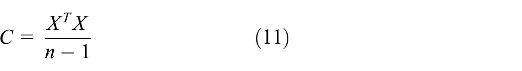
where X is the data matrix and n is the number of variable signals.

Next, C is subjected to eigenvalue decomposition. Projected into two subspaces, x can be expressed as

x = x_{e} + x_{r},

(12)

where x_e and x_r are the vectors of x projected into the principal component and residual subspace, respectively.

This results in x_r being expressed as

x_{r} = x (I - P P^{T}),

(13)

where the load matrix $P = [p_{1}, . ., p_{k}]$ , $P \in ℜ^{n \times k}$ . The matrix column denotes the eigenvectors that correspond to an eigenvector matrix’s first k columns.

Correspondence is established between the column eigenvectors and the nonnegative real eigenvalues, which are arranged as

λ_{1} \geq λ_{2} \geq \dots \geq λ_{n} \geq 0 .

(14)

where n is the number of component factors. STB selection is then performed to select a suitable scree test (ST, SST, or WST) for feature extraction.

On the basis of STB selection, x_r can be employed such that the test samples can be identified by indicator I, which is defined as

I = ‖ x_{r} ‖^{2} .

(15)

The hold-out procedure is employed by the SVM to determine the combination²⁴: parameter C and radial basis function kernel parameter γ. The grid-search strategy is used to determine the two parameters in SVM. Wang et al.²⁵ suggested trying exponentially growing sequencies of C (2⁻⁵, 2⁻³, …, 2¹⁵) and γ (2⁻¹⁵, 2⁻¹³, …, 2³) to identify good input parameters when the grid-search method is adopted. The different exponential values of C and γ are given to determine the combination (Table 1). In this study, each sample class {A, B, C} had 8640 data sets in each run for training the SVM model. The training samples constituted 720 data sets, and the remainders were applied in classification accuracy assessment. Table 1 lists accuracy test for different combinations of the two parameters. The SVM model used the following combination: C = 2⁹ and γ = 2⁻³ to obtain a high testing accuracy rate. The model with the combination was used for data detection because the classification outcomes would be optimal by using the proper parameter values in SVM.²⁶ For each training set, the eigenvalues $λ_{j}$ set can be iteratively determined using the dynamic STB selection scheme. Table 2 presents classification results of different ST schemes for k = 0, 1, 2 used sequentially by the SVM. Subsequently, optimal principal components can be identified by the WST (k = 2), after which the indicators I_i = {I₀, I₁, I₂} corresponding to classes {A, B, C} are obtained using the vectors projected into the residual subspace. Obtained on the basis of the residual subspace, the unknown indicator I can be further processed by indicators I_i and the SVM.

Table 1.

Testing accuracy for different combinations of parameter C and radial basis function kernel parameter γ, C (rows): value (5, …, 13) of log₂C, γ (columns): value (1, …, −7) of log₂γ.

C\γ	−7	−5	−3	-1	1
5	92	93	94	94	93
7	93	94	95	95	94
9	94	95	95	95	94
11	94	95	95	94	93
13	93	94	94	93	92

Table 2.

Classification results obtained using the SVM for different ST schemes.

Scheme\Accuracy (%)	A	B	C
ST	89	90	90
SST	91	91	92
WST	95	95	96

For adaptive data detection, the STB PCA algorithm applies the following steps:

Step 1: Input m samples and n features into the data sets X. Next, subject X to normalization (zero mean and unit variance).

Step 2: Subject the normalized X to PCA, thereby determining eigenvalues $λ_{j}$ .

Step 3: Perform STB selection in choosing a suitable ST for processing $λ_{j}$ .

Step 4: Establish the indicators I according to $λ_{j}$ for X.

Step 5: Classify I by using an SVM.

Step 6: Determine the accuracy rate, which is expressed as

Accuracy = \frac{N_{C}}{N}

(16)

where N_C is the number of sample classes in the test run that are correctly classified and N is the total number of test sets.

If the accuracy is greater than t [see (17)], then continue to step 7. If it does not exceed t, repeat steps 3–6.

t = T H_{i}

(17)

where the threshold values TH_i are sequentially set to range from 0.84 to 0.99 (inclusive): {TH_i} = {0.84, 0.81, 0.82, …, 0.99}, where i = 0, 1, 2, …, 15.

Step 7: Terminate the process. Conduct a suitable ST such that the classification results can be obtained, including the optimal principal components. The algorithm stops when any class does not fulfill the condition in step 6.

Detection of data by using dynamic STB PCA

The design and construction of the adaptive data detection system are presented as follows. The system uses a STB PCA algorithm that combines STB selection with SVM classification to detect air pollutants (Figure 3). The air pollutants can result in the highest values of air quality index (AQI) in different locations. Table 3 lists the highest AQI values (denoted AQI*) detected in locations A, B, and C. Data detection was conducted using the following steps.

Input 25 920 samples from the air pollutant measurement data.²⁷ Each sample had a data set containing information on the AQI and concentrations of various air pollutions, namely PM_2.5, PM₁₀, O₃, and CO (µg/m³), recorded hourly over 1 year in locations A, B, and C.

Detect the AQI* and the corresponding concentrations of PM_2.5, PM₁₀, O₃, CO (µg/m³).

Pop the detection data set and perform PCA.

Obtain the eigenvalues of the air pollution concentrations and execute the STB selection scheme.

According to the results of suitable STs, develop indicators.

Classify the indicators on the basis of the database I_i by using an SVM.

Determine the location and determine the corresponding AQI* and feature pollutants.

Figure 3.

Schematic of the steps taken by the detection system.

Table 3.

Highest AQI values (denoted AQI*) detected in locations A, B, and C. h_j: time interval; j: {0, 1, 2, …, 23} represents {0–1, 1–2, 2–3, …, 23–24 h}.

Month\Location	A	B	C (AQI*/h_j)
January	108/h₁₂	115/h₁₁	108/h₁₂
February	108/h₁₁	117/h₁₀	113/h₁₀
March	81/h₁₀	87/h₁₁	80/h₁₀
April	92/h₁₈	98/h₁₈	82/h₂₁
May	38/h₁₈	41/h₁₈	36/h₁₉
June	24/h₁₇	25/h₁₇	29/h₁₇
July	27/h₁₇	30/h₁₆	32/h₁₆
August	39/h₁₇	42/h₁₇	45/h₁₇
September	76/h₁₈	88/h₁₈	86/h₁₈
October	85/h₁₉	105/h₁₈	101/h₁₉
November	85/h₁₃	88/h₁₈	86/h₁₂
December	96/h₁₄	91/h₁₃	99/h₁₄

The STB PCA detection system (Figure 3) enabled adaptive data detection through the dynamic selection of suitable STs from the STB PCA algorithm (steps 3–5). Using the proposed method, the AQI* and feature pollutants in various locations were detected (steps 6 and 7).

Experimental results and discussion

Adaptive data detection was conducted with manufacturing and air pollution data as inputs to assess the performance and accuracy of our dynamic STB PCA method. The STB-PCA algorithm was applied, and combines STB selection with SVM.

Adaptive detection of manufacturing data using the STB PCA method

The STB PCA method was applied to supercapacitor manufacturing data. As shown in Table 4, each supercapacitor sample class had 128 validation samples for data detection testing. To evaluate the qualifications of the sample classes, a life test was performed: (1) Using a 1-A current, charge the supercapacitor to 2.70 V. (2) Wait 15 s. (3) Using a 1-A current, discharge the supercapacitor to 1.35 V. (4) Wait 15 s. (5) Perform steps 1–4 again. In the cycle test, the capacitance (F) and equivalent series resistance (mΩ), denoted Cap and ESR, respectively, were determined. Changes in these values were expressed as △Cap (%) and △ESR (%), respectively.

Table 4.

Classes of supercapacitor samples used in data detection.

Samples (ESR mΩ)	Class	Sample size	Training/Validation
50	A	256	128/128
60	B	256	128/128
70	C	256	128/128
55	D	256	128/128

Results of the cycle test performed on the supercapacitor sample classes are displayed in Figure 4. The average values for the testing samples are denoted {Cap, ESR}. Difficulty was encountered in distinguishing between classes {A, B, C, D} by using the data. Figure 5 presents the ST results of {Cap, △Cap, ESR, △ESR} for classes {B, D}. By using the STB PCA method and the WST scheme, the eigenvalues of component factors {PC2} and {PC3} were differentiated. Under the STB PCA method, certain principal components and their corresponding indicators were obtained (Table 5). The optimal results were the principal components for pc_j >1. Indicators I_i = {I₀, I₁, I₂, I₃} corresponded to the optimal principal components of classes {A, B, C, D}, namely {(pc₃, pc₄), (pc₁, pc₂, pc₃, pc₄), (pc₂, pc₃), (pc₁, pc₂, pc₄)}. Accuracy rates calculated in the detection of classes {A, B, C, D} by using certain indicators are shown in Table 6. With the mean accuracy being 95%, classes {A, B, C, D} were distinguishable by the indicators.

Figure 4.

Average (a) Cap and (b) ESR corresponding to classes {A, B, C, D} in the cycle test.

Figure 5.

ST results for the classes {B, D} and {PC1, PC2, PC3, PC4}. {B, D}: class samples obtained using PCA and ST scheme. {B*, D*}: class samples obtained using the STB PCA method and WST scheme. {PC1, PC2, PC3, PC4}: component factors.

Table 5.

Principal components with indicators obtained using the STB PCA method. pc_j: principal components; j: {1, 2, 3, 4} represents {Cap, △Cap, ESR, △ESR}, I_i (i = 0, 1, 2, 3): indicators for classes {A, B, C, D}.

Class	pc₁	pc₂	pc₃	pc₄	I_i
A	0.0006	0.2279	1.7923	1.7923	I ₀
B	1.0039	1.0039	1.8470	1.8470	I ₁
C	0.6917	1.6723	1.6723	0.0004	I ₂
D	1.0385	1.0385	0.0004	1.7805	I ₃

Table 6.

Accuracy rates obtained using indicators {(pc₃, pc₄), (pc₁, pc₂, pc₃, pc₄), (pc₂, pc₃), (pc₁, pc₂, pc₄)} to detect classes {A, B, C, D}. pc_j: principal components; j: {1, 2, 3, 4} represents {Cap, △Cap, ESR, △ESR}.

pc_j \ Accuracy (%)	A	B	C	D
pc₂, pc₃	84.0	84.0	94.9	83.4
pc₃, pc₄	94.5	92.2	70.3	73.4
pc₁, pc₂, pc₄	86.3	93.0	75.0	95.3
pc₁, pc₂, pc_3, pc₄	75.0	95.3	70.3	92.6

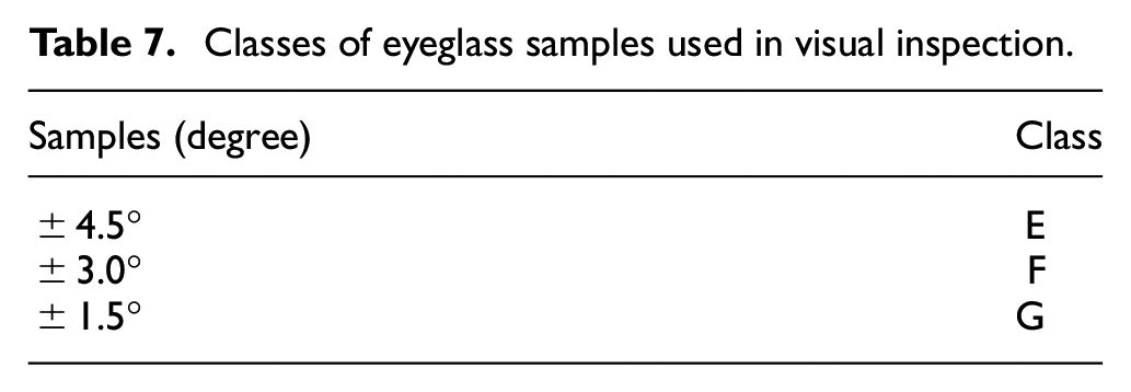
In addition to the data detection, the method was applied to mechanical inspection. The visual inspection in the experimental setup²³ was conducted to test the performance and accuracy of the method. Table 7 lists the classes of eyeglass samples including 512 samples used for classifier training, and other 512 samples used for testing accuracy. For inspection, an eyeglass with unknown features was affixed to a target panel, and the target panel-telescope was 10.67 m. The STB PCA method was employed to detect the digital camera-captured telescopic image. The algorithm selected the scheme {WST} and employed the indicators I_i = {I₀, I₁, I₂} (pc_j >1) corresponded to {(pc₁, pc₂, pc₃, pc₄, pc₅), (pc₁, pc₂, pc₃, pc₄, pc₅), (pc₁, pc₂, pc₃, pc₄)} to classify classes {D, E, F} (Table 8). Statistical approaches based on ensemble method²⁸ and Bayes classifier²⁹ were used to analyze the experimental results of data detection and visual inspection respectively. The ensemble method is given by

μ_{j} (x) = \frac{1}{L} \sum_{i = 1}^{L} d_{i, j} (x R_{i}), j = 1, . ., c .

(18)

where µ_j (x) is the confidence for each class. x is a given set of I_i. d_i,j(xR_i) is the probability assigned by the building classifier D_i. R_i is a rotation matrix of the features. L is the number of classifiers in the ensemble. c is the number of predicted classes. The unknown class can be identified as x assigned to the j class with the largest confidence. For Bayes classifier, the expression is given as follows

D (x) = - \frac{1}{2} \ln | C_{j} | - \frac{1}{2} [{(x - m_{j})}^{T} C_{j}^{- 1} (x - m_{j})]

(19)

where x is a set of I_i derived from an unknown class. The mean vectors m_j and covariance matrix C_j of the coefficients for the j class are then derived. The detection class can be recognized as the j class by minimizing the calculated value of D(x). The proposed method, in addition to attaining the highest accuracy rate in the data detection, exhibited superior classification performance in the visual inspection (Table 9).

Table 7.

Classes of eyeglass samples used in visual inspection.

Samples (degree)	Class
±4.5°	E
±3.0°	F
±1.5°	G

Table 8.

Principal components with indicators obtained using the STB PCA method in visual inspection. pc_j: principal components; I_i (i = 0, 1, 2): indicators for classes {E, F, G}.

Class	pc₁	pc₂	pc₃	pc₄	pc₅	I_i
E	1.4963	1.1357	1.0031	1.4963	1.1357	I ₀
F	1.5024	1.0865	1.3047	1.0042	1.0865	I ₁
G	1.3872	1.2032	1.3872	1.0017	0.3844	I ₂

Table 9.

Accuracy rates from the various methods in the experiments.

Experiment\Accuracy (%)	Ensemble method	Bayes classifier	The method
Data detection	91	84	95
Visual inspection	94	86	98

Detection system employing the STB PCA algorithm

The STB PCA algorithm was employed in assessing the performance and accuracy of the designed system (Figure 3). System evaluation was conducted using 25,920 samples of air-pollution data. Each sample in locations {A, B, C} had a corresponding data set consisting of hourly information on AQI and concentrations of PM_2.5, PM₁₀, O₃, and CO (µg/m³) recorded over 1 year. As training samples, 720 data sets recorded over 1 month in a single location were randomly selected. System evaluation was conducted using the remainder.

AQI* data for {PM_2.5, PM₁₀, O₃, CO} recorded in January, February, September, and October in locations {A, B, C} were subjected to a ST (Figure 6). For the data recorded in January and February (Figure 6(a) and (b)), the eigenvalues of component factor {PC2} could be differential from locations {A, B, C} by using the STB PCA algorithm. The algorithm selected the schemes {SST, WST} to distinguish between locations {A, B, C} for data recorded in {January, February}. Similarly, regarding the data recorded in September and October, the eigenvalues of component factor {PC2} were not distinguishable from locations {A, B, C}, as presented in Figure 6(c) and (d). The algorithm selected the schemes {SST, SST} to differentiate between locations {A, B, C} for the data recorded in {September, October}.

Figure 6.

ST results of AQI* data recorded in (a) January, (b) February, (c) September, and (d) October in locations {A, B, C}. {PC1, PC2, PC3, PC4}: component factors.

Table 10 lists the principal components with the selected schemes and indicators obtained using the STB PCA algorithm. The algorithm selected the schemes {SST, WST, SST, SST} and employed the indicators I_i = {I₀, I₁, I₂} (pc_j >1) in {January, February, September, October} to classify locations {A, B, C}. The indicators I_i were {(pc₁, pc₄), (pc₂, pc₃, pc₄), (pc₃, pc₄)}, {(pc₁, pc₃), (pc₂, pc₄), (pc₁, pc₃, pc₄)}, {(pc₃, pc₄), (pc₁, pc₂), (pc₁, pc₂)}, and {(pc₁, pc₂), (pc₃, pc₄), (pc₁, pc₂)}. Furthermore, the algorithm used the selected scheme to detect the AQI* feature pollutants in the same locations (Table 11): {(PM_2.5, CO), (PM₁₀, O₃, CO), (O₃, CO)}, {(PM_2.5, O₃), (PM₁₀, CO), (PM_2.5, O₃, CO)}, {(O₃, CO), (PM_2.5, PM₁₀), (PM_2.5, PM₁₀)}, and {( PM_2.5, PM₁₀), (O₃, CO), (PM_2.5, PM₁₀)}. The classification results of the 25 200 validation samples classified in locations A, B, and C are shown in Table 12. The mean accuracy was 95%, and the system used the algorithm to detect the samples (recorded hourly over 1 year). Due to the samples collected in only three locations, the performance of the classification model cannot be presented at all thresholds. For example, an ROC curve (receiver operating characteristic curve) can show the performance on a graph. This curve plots two parameters as (true positive rate, false positive rate).³⁰ In the study, (0.94, 0.023), (0.96, 0.025), and (0.95, 0.032) can be obtained by using the accuracy rate (equation (16)). To provide an aggregate information of performance across all possible classification thresholds, future works can employ the AUC (area under the ROC curve)³¹ to measure the entire two-dimensional area underneath the entire ROC curve, and to evaluate the classification model when samples in more locations are collected. Figure 7 presents a quantitative comparison of the system when using various learning algorithms. System performance achieved with three learning algorithms, namely the self-organizing map (SOM),³² backpropagation neural network (BPNN),³³ and K-nearest-neighbors (KNN),³⁴ respectively, was compared with that attained using our STB PCA approach. The procedures through which the algorithm parameters were selected are summarized as follows:

Table 10.

Principal components with the selected schemes and indicators obtained using the STB PCA algorithm. pc_j: principal components; j: {1, 2, 3, 4} presents AQI* data {PM_2.5, PM₁₀, O₃, CO}. I_i (i = 0, 1, 2): indicators for locations {A, B, C}.

Month	location	pc₁	pc₂	pc₃	pc₄	scheme	I_i
January	A	2.8942	0.1053	0.1053	1.0500	SST	I ₀
January	B	0.4140	2.5111	1.0500	2.5111	SST	I ₁
January	C	0.3152	0.3152	2.3280	1.3187	SST	I ₂
February	A	2.6232	0.3140	1.0175	0.0453	WST	I ₀
February	B	0.0749	2.0797	0.0749	1.0013	WST	I ₁
February	C	2.4494	0.3806	2.4494	1.0607	WST	I ₂
September	A	0.3985	0.3985	2.3591	1.0500	SST	I ₀
September	B	1.8914	1.0577	0.8294	0.2215	SST	I ₁
September	C	2.2914	1.1577	0.6294	0.6294	SST	I ₂
October	A	2.2868	1.1429	0.4277	0.4277	SST	I ₀
October	B	0.8980	0.8980	2.0135	2.0135	SST	I ₁
October	C	2.3135	1.0500	0.6088	0.2996	SST	I ₂

Table 11.

AQI* feature pollutants detected in locations A, B, and C by using the selected schemes.

Month\Location	A	B	C	scheme
January	PM_2.5, CO	PM₁₀, O₃, CO	O₃, CO	SST
February	PM_2.5, O₃	PM₁₀, CO	PM_2.5, O₃, CO	WST
March	PM_2.5, CO	PM_2.5, CO	PM_2.5, PM₁₀, O₃, CO	ST
April	O₃, CO	PM_2.5, O₃	PM₁₀	WST
May	N/A	N/A	PM_2.5	ST
June	O₃	PM₁₀	PM₁₀	SST
July	N/A	N/A	N/A	ST
August	PM_2.5, PM₁₀	PM_2.5, PM₁₀	PM_2.5, PM₁₀	ST
September	O₃, CO	PM_2.5, PM₁₀	PM_2.5, PM₁₀	SST
October	PM_2.5, PM₁₀	O₃, CO	PM_2.5, PM₁₀	SST
November	PM_2.5, PM₁₀, CO	PM_2.5, O₃	PM_2.5	ST
December	PM_2.5, CO	PM_2.5, O₃	PM₁₀, CO	WST

Table 12.

Classification results obtained using the STB PCA algorithm for classifying the air pollution samples in locations A, B, and C. T (rows): true values, P (columns): predicted values.

T\P	A	B	C
A	23,688	604	908
B	454	24,066	680
C	705	681	23,814

Figure 7.

Accuracy rates (in percentages) for various learning algorithms: SOM, KNN, BPNN, and SVM.

(1) Convert the input data of {I₀, I₁, I₂}. That is, the input vector, data set, and three neurons corresponding to {SOM, KNN, BPNN}. (2) Run the learning algorithms. The SOM network is trained using the Kohonen algorithm,³⁵ yielding an output layer consisting of three neurons ({A}, {B}, {C}). By taking a majority vote of the five nearest neighbors, the input data set is classified using the KNN algorithm. The class membership ({A}, {B}, {C}) constitutes the output layer. The BPNN trains a neural network with an input layer, hidden layer, and output layer containing three neurons, four neurons, and three neurons ({A}, {B}, {C}), respectively. (3) Obtain the accuracy rates corresponding to the output layers. For {SOM, KNN, BPNN, SVM}, they were 88%, 90%, 87%, and 95%, respectively. The results demonstrate that the proposed method has the highest accuracy. This is attributable to maximization of the distance between two classes within a feature space by the SVM. The performance of the BPNN on a certain issue depends on the data input.³⁶ The BPNN for detecting air pollutants may be sensitive to the input with noisy data and exhibits the worst performance. The computational complexity of learning algorithm was introduced in the experiment.³⁷ The amount of time necessary for an algorithm to complete binary searches is quantified by T(n). T(n) is given as

T (n) = O (\log n)

(20)

where O(log n) is the logarithmic time. The time that an algorithm requires for all inputs of size n is expressed in big O notation which excludes coefficients and lower-order terms. Using a time-cost function O(log n), the system evaluated various PCA-based methods, including the ST, SST, and WST schemes and the dynamic STB PCA approach. This function places a limit on the logarithmic time needed by a system for all n-sized inputs in big O notation. Moreover, it computes how much time an algorithm requires to execute binary search tree operations. The time-cost function and classification accuracy rates obtained are shown in Figure 8. The accuracy rate for our proposed method was highest among all PCA-based methods. For all the methods examined, the time-cost functions were lower than 45 μs. Overall, the dynamic STB PCA approach outperforms the ST, SST, and WST schemes.

Figure 8.

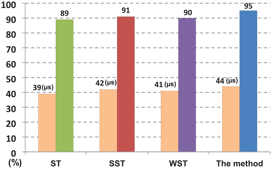
Comparison of algorithm performance under various PCA-based methods.

Conclusions

Herein, a dynamic STB PCA method was proposed for retaining the correct number of PCA components and for detecting various types of data. The proposed method was presented to improve PCA-technique performance when using insufficient or incorrect number of components. The proposed STB PCA learning algorithm employs a dynamic STB scheme combined with SVM for adaptive data detection, learning and training the input data sequence, and dynamically selects suitable STs through which the appropriate number of principal components was preserved. It is noted that the STB method provides suitable STs in PCA detection and improves the performance when classifying different data. The proposed detection system solves problems associated with using ambiguous standards on STs and effectively detects various types of data using the established suitable ST schemes. The results demonstrate that the designed system can successfully retain the correct number of PCA components, and adaptively detected manufacturing and air pollution data. The proposed method attained a data detection rate of 95%, 98%, and 95% for supercapacitor manufacturing data, visual inspection data, and air pollution data respectively. The proposed algorithm outperforms approaches in which ST, SST, and WST schemes are employed. To evaluate the classification model across all possible classification thresholds, further works on an aggregate measure of performance will be conducted based on the current study.

Footnotes

Appendix

Handling Editor: Chenhui Liang

Declaration of conflicting interests

The author(s) declared no potential conflicts of interest with respect to the research, authorship, and/or publication of this article.

Funding

The author(s) disclosed receipt of the following financial support for the research, authorship, and/or publication of this article: This work was supported in part from National Kaohsiung University of Science and Technology.

ORCID iD

Tsun-Kuo Lin

References

Zhao

Liu

Chen

, et al. Intelligent diagnosis using continuous wavelet transform and Gauss Convolutional Deep Belief Network. IEEE Trans Reliab. Epub ahead of print 13 June 2022. DOI: 10.1109/tr.2022.3180273

Yao

Guo

Deng

, et al. A novel mathematical morphology spectrum entropy based on scale-adaptive techniques. ISA Trans 2022; 126: 691–702.

Zhou

, et al. Parameter adaptation-based ant colony optimization with dynamic hybrid mechanism. Energy Appl Artif Intell 2022; 114: 105139.

Zhu

Keshtegar

Chakraborty

, et al. Novel probabilistic model for searching most probable point in structural reliability analysis. Comput Methods Appl Mech Eng 2020; 366: 113027.

Luo

Keshtegar

Zhu

, et al. Hybrid enhanced Monte Carlo simulation coupled with advanced machine learning approach for accurate and efficient structural reliability analysis. Comput Methods Appl Mech Eng 2022; 388: 114218.

Zhu

Keshtegar

Bagheri

, et al. Novel hybrid robust method for uncertain reliability analysis using finite conjugate map. Comput Methods Appl Mech Eng 2020; 371: 113309.

Zhu

Keshtegar

Ben Seghier

MEA

, et al. Hybrid and enhanced PSO: novel first order reliability method-based hybrid intelligent approaches. Comput Methods Appl Mech Eng 2022; 393: 114730.

Lin

Lee

Chen

, et al. Parameter determination of support vector machine and feature selection using simulated annealing approach. Appl Soft Comput 2008; 8: 1505–1512.

Lei

Shen

Wang

, et al. Real-time weld geometry prediction based on multi-information using neural network optimized by PCA and GA during thin-plate laser welding. J Manuf Process 2019; 43: 2007–2017.

10.

Gárate-Escamila

Hajjam

Hassani

Andrès

. Classification models for heart disease prediction using feature selection and PCA. Inform Med Unlocked 2020; 19: 100330.

11.

Levada

ALM

. Parametric PCA for unsupervised metric learning. Pattern Recognit Lett 2020; 135: 425–430.

12.

Mrówczyńska

Sztubecki

Greinert

. Compression of results of geodetic displacement measurements using the PCA method and neural networks. Measurement 2020; 158: 107693.

13.

Mehra

Bhatt

Kazi

, et al. Analysis of PCA based compression and denoising of smart grid data under normal and fault conditions. In: 2013 IEEE International Conference on Electronics, Computing and Communication Technologies (CONECCT), Bangalore, India, 17–19 January 2013, pp.1–6. New York: IEEE.

14.

Asadur Rahman

Foisal Hossain

Hossain

, et al. Employing PCA and t-statistical approach for feature extraction and classification of emotion from multichannel EEG signal. Egypt Inform J 2020; 21: 23–35.

15.

Pandey

Yadav

SKS

. Multi-objective optimization of vibration assisted electrical discharge drilling process using PCA based GRA method. Mater Today Proc 2020; 26: 2667–2672.

16.

Wang

Chen

, et al. Multi-objective optimization of vibration assisted electrical discharge drilling process using PCA based GRA method. Measurement 2020; 157: 107657.

17.

Priyanka Kumar

. Feature extraction and selection of kidney ultrasound images using GLCM and PCA. Procedia Comput Sci 2020; 167: 1722–1731.

18.

Zhang

, et al. Determination of key canopy parameters for mass mechanical apple harvesting using supervised machine learning and principal component analysis (PCA). Biosyst Eng 2020; 193: 247–263.

19.

Huang

. A combined method of cross-correlation and PCA-based outlier algorithm for detecting structural damages on a jacket oil platform under random wave excitations. Appl Ocean Res 2020; 102: 102301.

20.

Papandrea

Frigieri

Maia

, et al. Surface roughness diagnosis in hard turning using acoustic signals and support vector machine: A PCA-based approach. Appl Acoust 2020; 159: 107102.

21.

Allegretta

Marangoni

Manzari

, et al. Macro-classification of meteorites by portable energy dispersive X-ray fluorescence spectroscopy (pED-XRF), principal component analysis (PCA) and machine learning algorithms. Talanta 2020; 212: 120785.

22.

De Stefano

Ferrigno

Fontanella

, et al. A novel PCA-based approach for building on-board sensor classifiers for water contaminant detection. Pattern Recognit Lett 2020; 135: 375–381.

23.

Lin

. Adaptive principal component analysis combined with feature extraction-based method for feature identification in manufacturing. J Sens 2019; 2019: 5736104.

24.

Lin

. Dynamic weight-based learning method for data detection in manufacturing. Adv Mech Eng 2020; 12: 1–12.

25.

Wang

Zhang

. Support vector machines based on K-means clustering for real-time business intelligence systems. Int J Bus Intell Data Min 2005; 1: 54–64.

26.

Keerthi

Lin

. Asymptotic behaviors of support vector machines with Gaussian kernel. Neural Comput 2003; 15: 1667–1689.

27.

The Environmental Protection Administration. The measurement data of air pollutants, https://airtw.epa.gov.tw (2021, accessed 31 December 2021).

28.

Rodríguez

Kuncheva

Alonso

. Rotation forest: a new classifier ensemble method. IEEE Trans Pattern Anal Mach Intell 2006; 28: 1619–1630.

29.

Larsen

. Generalized naive Bayes classifiers. ACM SIGKDD Explor Newslett 2005; 7: 76–81.

30.

Fawcett

. An introduction to ROC analysis. Pattern Recognit Lett 2006; 27: 861–874.

31.

Hand

. Measuring classifier performance: A coherent alternative to the area under the ROC curve. Mach Learn 2009; 77: 103–123.

32.

Kodikara

GRL

McHenry

. Self-organizing maps for identification of zeolitic diagenesis patterns in closed hydrologic systems on the Earth and its implications for mars. Int J Sediment Res 2021; 36: 567–576.

33.

Zhao

Yang

, et al. Prediction of temperature and CO concentration fields based on BPNN in low-temperature coal oxidation. Thermochim Acta 2021; 695: 178820.

34.

Xiong

Yao

. Study on an adaptive thermal comfort model with K-nearest-neighbors (KNN) algorithm. Build Environ 2021; 202: 108026.

35.

Sujeet

Shankar

SVS

Subramaniyaswamy

. A hypergraph based Kohonen map for detecting intrusions over cyber–physical systems traffic. Future Gener Comput Syst 2021; 119: 84–109.

36.

. Advantages and disadvantages of using artificial neural networks versus logistic regression for predicting medical outcomes. J Clin Epidemiol 1996; 49: 1225–1231.

37.

Schonhage

. Equation solving in terms of computational complexity. In: Proceedings of the international congress of mathematicians, Berkeley, CA, 3–11 August 1986, pp.131–153. Providence, RI: American Mathematical Society.

Dynamic ST-based PCA method for adaptive data detection

Abstract

Keywords

Introduction

Related work

Proposed method

Dynamic STB PCA method

PCA and the dynamic STB selection scheme

STB PCA algorithm and SVM classification

Detection of data by using dynamic STB PCA

Experimental results and discussion

Adaptive detection of manufacturing data using the STB PCA method

Detection system employing the STB PCA algorithm

Conclusions

Footnotes

Appendix

Declaration of conflicting interests

Funding

ORCID iD

References