Dynamic weight-based learning method for data detection in manufacturing

Abstract

In this study, a dynamic weight-based method combined with principal component analysis (PCA) was developed for the first time for detecting measurement data in manufacturing. This weight-based learning technique can learn and train the measurement data sequence to isolate incorrect data sources for achieving high accuracy when detecting various types of data. Research has revealed that unsuitable image or data features might cause poor performance in industrial inspections. In contrast to the previous inspection methods, the weight-based learning method proposed in this study employs a dynamic learning algorithm for effectively and adaptively selecting optimal principle components to the support vector machine (SVM) algorithm and then establishes indicators. Finally, these PCA-based indicators act as substitutes for massive amounts of data in data processing and can be applied to timely detect data when the data contain redundant and incorrect inputs in a sequence. The experimental results indicate that the proposed method, which combines dynamic weight-based feature extraction with PCA, can provide useful indicators for detecting various types of manufacturing data and exhibited satisfactory performance in the data detection.

Keywords

Data detection principal component analysis support vector machine weight-based learning method

Introduction

A wide range of techniques are applied in industrial automation for enabling automatic operation of manufacturing processes and reducing human operators. A set of tools, such as computer software and machinery, are required for industrial automation. They incorporate different devices and systems that impact aspects of the manufacturing processes. Monitoring the motion process of machinery is commonly used method¹ for improving product quality in manufacturing, but an effective qualification test-based method for identifying qualified products has yet to be developed. There are still some defects of the qualification test in manufacturing: (1) test data provide insufficient information on current test conditions, (2) test data obtained from measurements might include redundant or incorrect inputs for data processing, and (3) data processing requires considerable time and causes poor manufacturing performance. Therefore, the data detection method for solving these problems is of great significance. Researches have suggested various optimized control strategies for industrial automatic control systems.^2–4 Data-driven methods based on data processing can diagnose fault conditions in systems.^5,6 These methods use historical measurement data of various test conditions for determining the essential correlations between variables and parameters. However, new issues arise in the time consumption in data processing and the operating costs when data processing units break down and provide inaccurate readings. What kind of feature extraction can describe the data information of the qualification test in manufacturing? How to deal with the data feature to timely classify the qualified products has become a challenge. A data-driven multivariate statistical process (MSP) method has been widely used to extract the data feature for further establishing classification model, such as principal component analysis (PCA).^7,8 However, MSP might hardly establish an accurate and reliable model because it is pre-assumed that the data follow Gaussian distribution. Unlike traditional MSP, a dynamic weight-based method coupled with PCA is proposed to solve the issue. In this manner, the main contributions of this paper can be highlighted as follows: (1) The weight-based learning method is an extraction tool, which learns and trains the measurement data sequence to isolate incorrect data sources. (2) The dynamic weight-based scheme is an effective tool for effectively and adaptively selecting optimal principle components to the support vector machine (SVM) algorithm and then establishes indicators. (3) These PCA-based indicators act as substitutes for massive amounts of data on various test conditions in data processing and can be applied to timely detect data when the data contain redundant and incorrect inputs in a sequence. The results of the proposed methods show satisfactory classification performance in the data detection.

The rest of this paper is structured as follows. The related studies are reviewed in Section 2. The proposed method for establishing PCA-based indicators to detect various types of measurement data in manufacturing is described in Section 3. The experimental results determined through the PCA-based detection system are provided in Section 4, which also presents a comparison between the proposed method and existing methods. The conclusions of this study are presented in Section 5.

Related work

The aforementioned literatures have proved that PCA is an effective variable reduction technique and have successfully used PCA to establish detection models for data-driven prediction, data-based estimation, and fault detection. Hosseinpour et al.⁹ used an iterative network-based fuzzy partial least squares (INFPLS) model combined with PCA to determine the higher heating value of biomass fuels as a function of the fixed carbon content. To obtain the required background data for the INFPLS model, the aforementioned authors used PCA to eliminate the experimental data’s collinearity. Manoharan et al.¹⁰ developed a data-based predictive method on the basis of PCA to predict the wire bond time to failure for plastic encapsulated components. Uddin et al.¹¹ used a PCA-based assessment for identification of vulnerable areas in Bangladesh’s coastal region. Moreover, PCA is considered as a novel technique for fault detection and diagnosis.^12–14 Wu et al.¹⁵ proposed a statistical method based on PCA for fault detection and the assessment of the gas supply in solid oxide fuel cell systems. They collected data for a real system and used the aforementioned method to conduct fault detection. Li and Hu¹⁶ employed ensemble empirical mode decomposition (EEMD) denoising to develop a PCA-based method for detecting sensor faults. The EEMD-PCA method developed by the aforementioned authors outperformed PCA for eight critical sensors. To detect and isolate sensor faults in a nuclear power plant, Li et al.¹⁷ used an improved PCA method. The practical performance of this method was improved by combining the PCA method with false alarm reduction and data preprocessing methods.

In contrast to previous studies on PCA, this study proposed a dynamic weight-based data processing framework to deal with redundant or incorrect inputs in measurement data. The proposed technique can adaptively detect measurement data under varying test conditions on the basis of the SVM algorithm to establish PCA-based indicators. Thus, models established on the basis of the measurement data, which are obtained by using the traditional PCA method, cannot be directly applied to different test conditions. The proposed dynamic weight-based learning method can learn and train the measurement data sequence to solve the aforementioned issue for identifying products in a timely manner by using the established PCA-based indicators.

Proposed method

Dynamic weight-based data processing framework

A data processing framework derived from image identification scheme¹⁸ was proposed to dynamically select optimal PCA-based weights for data detection.

Figure 1 presents a schematic of the weight-based processing framework. The weight-based learning method can identify measurement data by using the PCA-based training strategy on the basis of SVM classification results. The procedure of data identification is described in the following text.

(1) Data preprocessing: First, the measurement data are input. To execute the data processing framework, some samples are selected randomly as the training samples for each dataset to train the PCA model, and the remaining samples are used to conduct PCA-based selection for evaluating the model accuracy.

(2) Weight-based data processing: Data feature extraction is executed on the basis of PCA. In PCA, eigenvalue decomposition is conducted to obtain eigenvectors and eigenvalues for representing the variation in the data features. Eigenvalue decomposition generates projection vectors in the residual and principal component subspaces. The residual subspace is used to identify the test data. After eigenvalue decomposition, a scree test is used to identify the optimal principal components. The weight-based learning method based on the scree test is described in the following text.

Figure 1.

Schematic of the dynamic data processing framework.

The threshold $δ$ is proposed to dynamically adjust the eigenvalues.

δ (λ_{i, j}), i = 0, 1, . ., n - 1, j = 1, 2, . ., n

(1)

where $λ_{i, j}$ represents the eigenvalues of the projection vectors in the residual subspace, n represents the number of principal components, i is set from 0 to n-1 for the number of features, and j is set from 1 to n for the number of component factors. If $λ_{i, j}$ is greater than 0.5 but less than 1 (0.5 < $λ_{i, j}$ < 1), then $δ$ is equal to $λ_{i, j}$ and retains the eigenvalues; otherwise, $δ$ = 0 and the eigenvalues ae eliminated.

The weight $ω_{i, j}$ is proposed for adjusting the $δ$ value.

ω_{i, j} = 1 + t_{i}

(2)

where the adjustable value t_i is set to have a value of 0.01–0.99 sequentially and {t_i} = {0.01, 0.02, 0.03, …, 0.99}, i = 0, 1, 2, …98.

The new eigenvalues $λ_{i, j}^{*}$ can be calculated as follows:

λ_{i, j}^{*} = ω_{i, j} \times δ (λ_{i, j}) for 0.5 < λ_{i, j} < 1,

(3)

and

λ_{i, j}^{*} = λ_{i, j} for λ_{i, j} \geq 1

(4)

The optimal eigenvalues $λ_{i, j}^{*}$ can be obtained by using the scree test combined with SVM classification (Section 3.2). The scree test is described in the following text.

S_{cr} (λ_{i, j}^{*})

(5)

where the parameter S_cr is used to decrease the number of principal components and identify the optimal components. If $λ_{i, j}^{*}$ > 1, S_cr is equal to 1 and retains the component; otherwise, S_cr is equal to 0 and the component is eliminated.

(3) PCA model training: The eigenvalues of each training dataset can be calculated iteratively through weight-based data processing. After the iterative calculation of the eigenvalues, the corresponding optimal principal components are determined and then the optimal data features are obtained.

(4) PCA-based selection: After weight-based data processing, the eigenvalues of each test dataset can be obtained. Subsequently, the optimal principal components are determined using the scree test. The corresponding eigenvalues, which are obtained using the scree test, can be processed through indicator establishment and SVM classification.

(5) Indicator establishment and SVM classification: Indicators are established on the basis of the projection vectors in the residual subspace. SVM is then employed to determine whether the data features belong to a certain pattern. The SVM algorithm performs indicator identification on the basis of the indicators obtained through the training of the PCA model. If the accuracy rate obtained from the SVM classification exceeds a given accuracy threshold t, the process is terminated, and then the optimal principal components and corresponding optimal data features are obtained; otherwise, the weight used in the weight-based data process is reset and the procedure is repeated. Moreover, the procedure stops if any test data point does not satisfy the condition in the SVM classification. The accuracy threshold t can be expressed as follows:

t = T_{i}

(6)

where T_i is set in the range 0.80–0.99 sequentially and {T_i} = {0.80, 0.81, 0.82, …, 0.99}, i = 0, 1, 2, …, 19.

Weight-based learning algorithm

This section describes the proposed weight-based learning algorithm, which involves PCA, weight-based learning, and SVM classification.

PCA involves converting a set of possibly correlated data into a set of uncorrelated data to reduce data dimensionality. The proposed weight-based learning algorithm, which combines PCA with the weight-based learning method, can provide optimal eigenvalues for representing data features. This algorithm can transform correlated high-dimensional data features to uncorrelated low-dimensional data features. The PCA model consists of the original data that comprises m raw samples (rows) for n variable signals (columns). This model can be expressed in the matrix form (X; X $\in ℜ^{m \times n}$ ) as follows:

X = {[\begin{matrix} x_{11} & \dots & x_{1 n} \\ ⋮ & ⋱ & ⋮ \\ x_{m 1} & \dots & x_{mn} \end{matrix}]}_{m \times n}

(7)

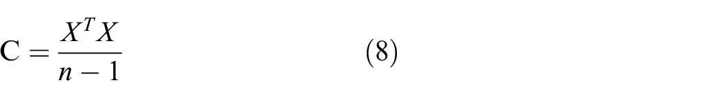
The covariance matrix C of the matrix X demonstrates correlation and is defined as follows:

C = \frac{X^{T} X}{n - 1}

(8)

Eigenvalue decomposition of the covariance matrix C is performed. Then x can be projected onto two subspaces and expressed as follows:

x = x_{e} + x_{r},

(9)

where x_e and x_r are the projection vectors of x in the residual and principal component subspaces, respectively. The parameter x_r is expressed as follows:

x_{r} = x (I - P P^{T}),

(10)

where $P = [p_{1}, . ., p_{k}]$ , $P \in ℜ^{n \times k}$ . The columns of the load matrix P contain the eigenvectors corresponding to the former column k largest eigenvalue of the covariance matrix C. The column eigenvectors correspond to non-negative real eigenvalues. The corresponding eigenvalues have the following order:

λ_{1} \geq λ_{2} \geq \dots \geq λ_{n} \geq 0 .

(11)

The parameter x_r can be employed to determine the indicator S for identifying the data features. The indicator S is defined as follows:

S = ‖ x_{r} ‖^{2} .

(12)

Figure 2 illustrates the procedure of the proposed weight-based learning algorithm, which combines the PCA-based weight learning method with the SVM algorithm to dynamically select optimal weights for data detection. In the SVM algorithm, the radial basis function kernel parameter γ and the parameter C should be optimized.¹⁹ The aforementioned parameters were determined using the hold-out procedure in this study. Each run involved the use of 256 datasets for each sample class to train the SVM model. In the hold-out procedure, 128 datasets were selected randomly as the training samples, and the remaining datasets were used for evaluating the accuracy of SVM classification. When C was set as 2¹¹ and γ was set as 2⁻³ in the SVM model, a high SVM classification accuracy was obtained. The classification results obtained with the aforementioned parameter values for different sample sizes are listed in Table 1, which indicates that similar classification results were obtained for 256, 512, and 1024 samples.

Figure 2.

Flowchart of the weight-based learning algorithm.

Table 1.

Classification results with the combination for different sample sizes for each sample class.

Sample size	Training	Validation	Accuracy rates (%)
32	16	16	94
64	32	32	92
128	64	64	94
256	128	128	95
512	256	256	95
1024	512	512	95

In the proposed approach, the following steps are adopted to select optimal weights dynamically for effective data detection:

Step 1: Input the test dataset X₀ and training dataset X₁, which comprise m samples and n features. Normalize the X₀ and X₁ with zero mean and unit variance.

Step 2: Execute PCA for the normalized X₀ and X₁ and obtain the corresponding eigenvalues ( $λ_{i, j}$ ).

Step 3: Set the number of features i (i = {0, 1, 2, 3, …, n-1} sequentially) and number of component factors j (j = {1, 2, 3, …, n} sequentially). Then, set the weight $ω_{i, j}$ (2).

Step 4: Calculate the new eigenvalues ( $λ_{i, j}^{*}$ ) by using (3) and (4).

Step 5: Employ the scree test S_cr to reduce the number of principal components and identify the optimal components.

Step 6: Determine the indicators S and S_i for X₀ and X₁, respectively.

Step 7: Classify the indicator S on the basis of S_i by using an SVM.

Each S_i value is obtained through PCA model training. For sample class {A, B, C, D}, the indices i = (0, 1, 2, 3) correspond to the indicators {S₀, S₁, S₂, S₃}. Every indicator has 128 samples for every training dataset. The training process involves the following steps: (1) input X₁, (2) normalize X₁, (3) execute PCA to obtain $λ_{i, j}$ , (4) set the weight $ω_{i, j}$ and calculate the new eigenvalues $λ_{i, j}^{*}$ , (5) identify the optimal principal components according to the SVM model and S_cr, (6) determine S_i according to the optimal principal components, (7) determine the accuracy rate, and (8) terminate the training process and obtain the optimal principal component PC_j (j= {1, 2, 3, …, n}) and its the corresponding data feature f_i (i = {0, 1, 2, 3, …, n-1}).

The accuracy rate is defined as follows:

Accuracy = \frac{N_{C}}{N}

(13)

where N_C is the number of correctly classified sample classes in the test run, and N is the total number of test datasets (N is 128 in this study). If the accuracy rate is higher than a certain accuracy threshold t (6), Step 8 is conducted; otherwise, the weight $ω_{i, j}$ is reset and Steps 4–8 are repeated. Moreover, the algorithm is terminated when a sample class does not satisfy the condition in Step 8.

Data detection system using PCA-based indicators

A detection system was designed and constructed for measurement data detection in supercapacitor manufacturing (Figure 3).

Figure 3.

The detection system.

The system uses a dynamic weight-based method combined with PCA to establish PCA-based indicators for detecting the measurement data. Table 2 presents the supercapacitor sample classes used in the experiments. The qualification of the sample classes was examined by performing a cycle test as follows:

Step 1: Charge the supercapacitor to 2.70 V by using a 1-A current source.

Step 2: Wait for 15 s.

Step 3: Discharge the supercapacitor to 1.35 V by using a current of 1 A.

Step 4: Wait for 15 s.

Step 5: Repeat Steps 1–4.

Table 2.

Classes of supercapacitor samples used in the experiments.

Samples (ESR mΩ)	Class
50	A
60	B
70	C
55	D

The capacitance [Cap (F)] and the equivalent series resistance [ESR (mΩ)] were measured in the cycle test. The changes in the Cap (△Cap) and ESR (△ESR) were derived as follows.

Δ Cap = \frac{(Cap - iCap)}{iCap} \times 100 %

(14)

Δ ESR = \frac{(ESR - iESR)}{iESR} \times 100 %

(15)

where iCap and iESR are the initial measured values of the Cap and ESR, respectively.

The detection system (Figure 3) detected data by employing the PCA-based indicators, which were obtained from the weight-based learning algorithm (Figure 2). The first two steps in the detection procedure are as follows: (1) set {PC_j, f_i} and (2) determine {Q} (measured data queue of testing samples, {Q} = {Cap, △Cap, ESR, △ESR}). If {Q} is not empty, Step 3 is performed; otherwise, the process is terminated. The remaining steps in the detection procedure are as follows: (3) begin the iterative procedure from Q₀ (initial measured data queue of the testing samples) by popping a measured data queue from {Q}, (4) normalize the measured data queue, (5) perform PCA to obtain the eigenvalues, (6) set the weight and calculate the new eigenvalues, (7) use the scree test to identify the optimal principal components, and (8) determine S and classify it according to S_i by using the SVM. The parameter S_i is obtained through PCA model training conducted for {PC_j, f_i}. For example, to detect the sample class A in {Q}, PC_j and f_i are set as {PC₃, PC₄} and {f₂, f₃}, respectively. The iterative procedure is started from Q₀ by popping a measured data queue from {Q}. Each procedure involves PCA, determining the weight and eigenvalues, the scree test, indicator establishment, and indicator classification by using the SVM. The iterative procedure is completed when {Q} does not comprise any data queues. Subsequently, for detecting another class, PC_j and f_i are reset and {Q} is selected for detection. The detection is complete when {Q} is empty.

Experimental results and discussion

This section describes the use of the designed system for measurement data detection in supercapacitor manufacturing. Experiments were performed for examining the performance and accuracy of the dynamic weight-based learning method. The results indicate that the weight-based learning algorithm can be used to establish PCA-based indicators for detecting measurement data in a system. The designed system, which combines dynamic weight-based feature extraction with the SVM algorithm for adaptively classifying data samples, can detect samples efficiently by using PCA-based indicators.

Weight-based learning method for measurement data detection

This section describes the use of the weight-based learning method for detecting measurement data in supercapacitor manufacturing. To test the data detection, samples were selected from the 128 validation samples for each class (Table 2). The designed system (Figure 3) used a dynamic weight-based learning method combined with PCA for detecting the measurement data.

Figure 4 displays the cycle test results for the classes of supercapacitor samples. The set {Cap, △Cap, ESR, △ESR} represents the average values of the testing samples in the cycle test. Figure 5 depicts the scree test results of {Cap, △Cap, ESR, △ESR} for sample class {A, B, C, D}. The component factor {PC2} for the class {B, D} was distinguished from component factor {PC3} by using the dynamic weight-based learning method. Table 3 lists the principal components and PCA-based indicators, which were obtained by using the dynamic weight-based learning method combined with PCA.

Figure 4.

The average values of: (a) Cap, (b) △Cap, (c) ESR, and (d) △ESR for the class {A, B, C, D} in the cycle test.

Figure 5.

The scree test results for class {A, B, C, D}, {PC1, PC2, PC3, PC4}: the component factors, {A, B, C, D}: class samples by using the PCA algorithm, {A*, B*, C*, D*}: class samples by using the dynamic weight-based PCA algorithm.

Table 3.

The principal components with PCA-based indicators obtained using the PCA-based methods.

Class	pc₁	pc₂	pc₃	pc₄	S_i
A	0.0006	0.2279	1.7923	1.7923	S ₀
A*	0.0006	0.2279	1.7923	1.7923	S ₀*
B	0.5770	0.5770	1.8470	1.8470	S ₁
B*	1.0039	1.0039	1.8470	1.8470	S ₁*
C	0.6917	1.6723	1.6723	0.0004	S ₂
C*	0.6917	1.6723	1.6723	0.0004	S ₂*
D	0.5920	0.5920	0.0004	1.7805	S ₃
D*	1.0385	1.0385	0.0004	1.7805	S ₃*

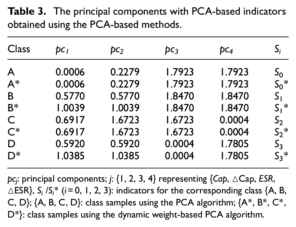
pc_j: principal components; j: {1, 2, 3, 4} representing {Cap, △Cap, ESR, △ESR}, S_i /S_i* (i = 0, 1, 2, 3): indicators for the corresponding class {A, B, C, D}; {A, B, C, D}: class samples using the PCA algorithm; {A*, B*, C*, D*}: class samples using the dynamic weight-based PCA algorithm.

The principal components {pc₁, pc₂} for class {B, D} were adjusted using the dynamic weight-based learning method (pc_j >1). The principal components for pc_j >1 were the optimal selections. The indicators S_i* = {S₀^*, S₁^*, S₂^*, S₃^*} were obtained by using the aforementioned method for class {A, B, C, D}. Table 4 lists the data features obtained using the dynamic weight-based method for class {A, B, C, D}. The data features {Cap, △Cap, ESR, △ESR} and {Cap, △Cap, △ESR} were appropriate selections for class {B, D} because these features could be distinguished from each other. The principal components {(pc₃, pc₄), (pc₁, pc₂, pc₃, pc₄), (pc₂, pc₃), (pc₁, pc₂, pc₄)} were the PCA-based indicators (S_i* = {S₀^*, S₁^*, S₂^*, S₃^*}) of class {A, B, C, D} because these components had high accuracy rates for class {A, B, C, D} (Table 5).

Table 4.

The data features obtained using the dynamic weight-based method for the class {A, B, C, D}.

Class	f ₀	f ₁	f ₂	f ₃
A	N/A	N/A	ESR	△ESR
B	Cap	△Cap	ESR	△ESR
C	N/A	△Cap	ESR	N/A
D	Cap	△Cap	N/A	△ESR

f _i : data features, i: {0, 1, 2, 3} representing {Cap, △Cap, ESR, △ESR}.

Table 5.

Accuracy rates using the principal components for detecting the class samples.

pc_j\Accuracy (%)	A	B	C	D
pc₁	14.1	21.8	23.4	22.7
pc₂	18.0	22.7	70.3	24.2
pc₃	71.1	72.7	69.5	10.2
pc₄	71.1	71.9	10.9	93.8
pc₁, pc₂	33.6	32.0	72.7	32.0
pc₂, pc₃	84.0	84.0	94.9	83.4
pc₃, pc₄	94.5	92.2	70.3	73.4
pc₁, pc₂, pc₄	86.3	93.0	75.0	95.3
pc₁, pc₂, pc_3, pc₄	75.0	95.3	70.3	92.6

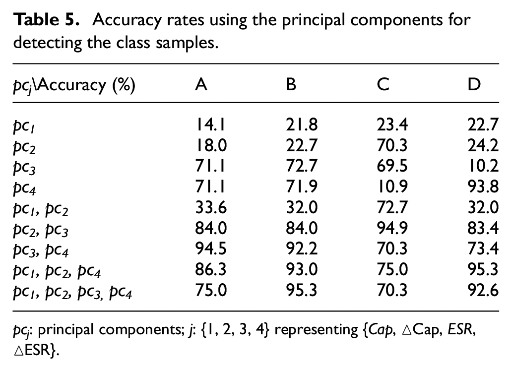
pc_j: principal components; j: {1, 2, 3, 4} representing {Cap, △Cap, ESR, △ESR}.

Data detection using PCA-based indicators in manufacturing

This section describes the life test conducted for supercapacitor manufacturing to determine suitable PCA-based indicators. Table 6 lists the sample classes for detection. The samples used in the life test were selected from the 128 validation samples for each class (Figure 6). Figure 6 illustrates the procedure of the life test. Cap (F), ESR_a (mΩ), and ESR_b (mΩ) were measured in the life test. ESR_a (mΩ) and ESR_b (mΩ) were measured using a type A circuit and type B circuit respectively. The parameters △Cap, △ESR_a, and △ESR_b were derived using (14) and (15).

Table 6.

Classes of supercapacitor samples used in the life test.

Samples (ESR_a mΩ)	Class
22	E
19	F
20	G
21	H
18	I

ESR_a: the equivalent series resistance measured using the type A-circuit.

Figure 6.

Procedure of the life test.

Figure 7 displays the average values of △Cap, ESR_a, ESR_b, △ESR_a, and △ESR_b for class {E, F, G, H, I} in the life test of supercapacitor manufacturing. The class {E, F, G, H, I} was difficult to distinguish from the other classes on the basis of the aforementioned values. Table 7 lists the adjusted principal components obtained using the dynamic weight-based learning method. The adjusted principal components for pc_j >1 were the optimal selections. The indicators {S₅^*, S₇^*} were obtained for class {F, H} by using the aforementioned method.

Figure 7.

The average values of (a) △Cap, (b) ESR_a, (c) △ESR_a, (d) ESR_b, and (e) △ESR_b for the class {E, F, G, H, I} in the life test.

Table 7.

The adjusted principal components obtained by the dynamic weight-based learning method.

Class	pc₁	pc₂	pc₃	pc₄	pc₅	S_i
E	0.0187	0.5920	0.0004	1.7805	0.5920	S₄
F	0.0093	0.0110	0.5234	0.0232	1.9301	S₅
F*	0.0093	0.0110	1.0049	0.0232	1.9301	S₅*
G	0.0261	0.0303	0.4977	0.0683	1.9356	S₆
H	1.9340	0.0098	0.5091	1.9340	0.0227	S₇
H*	1.9340	0.0098	1.0029	1.9340	0.0227	S₇*
I	1.9120	0.0217	0.0208	1.9120	0.0540	S₈

pc_j: principal components; j: {1, 2, 3, 4, 5} representing {△Cap, ESR_a, ESR_b, △ESR_a, △ESR_b }; S_i /S_i* (i = 4, 5, 6, 7, 8): indicators for the corresponding class {E, F, G, H, I}; {E, F, G, H, I}: class samples with the principal components; {F*, H*}: class samples with the adjusted principal components.

Figure 8 displays the scree test results for class {F, H}. The adjusted component factor {PC2} for class {F, H} could be clearly distinguished from component factor {PC3}. Table 8 lists the data features of class {E, F, G, H, I} for the indicators {S₄, S₅*, S₆, S₇*, S₈}. The indicators with the data features {(△ESR_a), (ESR_b, △ESR_b), (△ESR_b), (△Cap, ESR_b, △ESR_a), (△Cap, △ESR_a)}, which are denoted as {(f₃), (f₂, f₄), (f₄), (f₀, f₂, f₃), (f₀, f₃)}, were the optimal selections for class {E, F, G, H, I}. The results for detecting class {E, F, G, H, I} when using the PCA-based indicators {S₄, S₅*, S₆, S₇*, S₈} with the optimal principles {(PC₄), (PC₃, PC₅), (PC₅), (PC₁, PC₃, PC₄), (PC₁, PC₄)} are displayed in Table 9. An average accuracy rate of 95% was obtained for detecting class {E, F, G, H, I}.

Figure 8.

The scree test results for class {F, H}, {PC1, PC2, PC3, PC4, PC5}: the component factors, {F, H}: class samples with component factors, {F*, H*}: class samples with adjusted component factors.

Table 8.

The data features of class {E, F, G, H, I} for the corresponding indicators {S₄, S₅*, S₆, S₇*, S₈ }.

S_i	f ₀	f ₁	f ₂	f ₃	f ₄
S₄	N/A	N/A	N/A	ESR_b	N/A
S₅*	N/A	N/A	△ESR_a	N/A	△ESR_b
S₆	N/A	N/A	N/A	N/A	△ESR_b
S₇*	△Cap	N/A	△ESR_a	ESR_b	N/A
S₈	△Cap	N/A	N/A	ESR_b	N/A

f_i: data features; i: {0, 1, 2, 3, 4} representing {△Cap, ESR_a, ESR_b, △ESR_a, △ESR_b}.

Table 9.

Classification results using the PCA-based indicators for detecting the class samples, T (rows): true values, P (columns): predicted values.

T\P	E	F	G	H	I	PC_j	S_i
E	121	0	1	2	4	PC₄	S₄
F	1	122	3	1	1	PC₃, PC₅	S₅
G	1	4	121	1	1	PC₅	S₆
H	2	0	0	122	4	PC₁, PC₃, PC₄	S₇
I	2	0	1	3	122	PC₁, PC₄	S₈

PC _j (j = 1,2,3,4,5): optimal principle components; S _i (i = 0,1,2,3,4): (i = 4, 5, 6, 7, 8): indicators for the corresponding class {E, F, G, H, I}.

To evaluate the designed detection system, various classification methods were used to detect the sample classes. The classification performance of learning classifiers based on the SVM, K-nearest neighbor (KNN),^20,21 and back propagation neural network (BPNN),^22,23 algorithms were compared with that of the proposed method. The input dataset in KNN classification was {S₄, S₅, S₆, S₇, S₈}, and the output dataset in this classification was the class membership ({E}, {F}, {G}, {H}, {I}). Input data classification was performed according to the majority vote of their k = 5 nearest neighbors of a data point. The BPNN used in this study was a neural network that comprised an input layer containing five neurons ({S₄, S₅, S₆, S₇, S₈}), an output layer containing five corresponding neurons ({E}, {F}, {G}, {H}, {I}), and a hidden layer containing seven corresponding neurons. The steps in the algorithms are as follows: (1) Input the 128 validation samples for each class {E, F, G, H, I} from the sample queue, (2) set the number of features i (i = {0, 1, 2, 3, …, n-1} sequentially) and number of principal components j (j = {1, 2, 3, …, n} sequentially) for each class {E, F, G, H, I}, (3) execute the dynamic weight-based PCA algorithm and SVM classification, and then denote the obtained results as {the method}, (4) use the PCA algorithm with the SVM, KNN, and BPNN algorithm individually and denote the results as {SVM, KNN, BPNN}, and (5) determine if the sample queue comprises any sample. A time-cost function O(log n), which bounds the logarithmic time required by an algorithm for all n-sized inputs in the big-O notation, was also used to evaluate the designed system. The parameter O(log n) can quantify the time required by an algorithm to complete binary search tree operations. Figure 9 displays the O(log n) values (μs) and accuracy rates (%) obtained in class detection.

Figure 9.

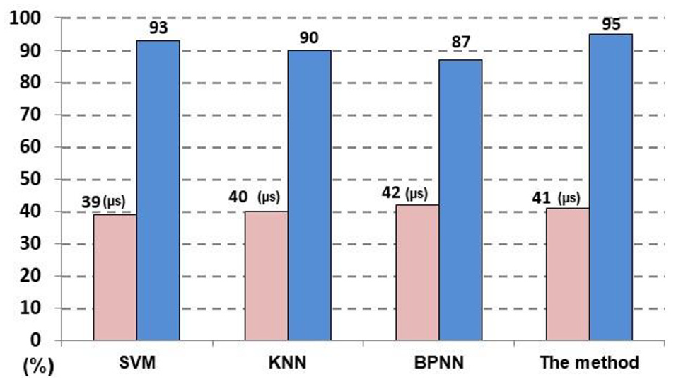
The O(log n) (µs) and accuracy rates (%) obtained in class detection.

The following accuracy rates were obtained: 93% for the SVM algorithm, 90% for the KNN algorithm, 87% for the BPNN algorithm, and 95% for the proposed method. The aforementioned four methods required almost the same time for classifying samples. The SVM-based methods (the SVM algorithm and proposed method) and KNN-based method exhibited high classification performance because these methods are advantages for solving problems with insufficient samples. However, the proposed method (accuracy rate: ≧95%) outperformed the other three methods that employ PCA without adjustable PCA-based indicators. Furthermore, more experiments were performed to evaluate the dynamic weighting’s performance in data detection. The experiment setup¹⁸ was applied to the identification of suitable image features. Table 10 lists the classes of test samples used in the experiments. Samples were chosen from 512 validation samples for each class. For detection, an object (wrench / eyeglass) with unknown features was affixed to a target panel. The distance between a target panel and a telescope was 10.67 m. The platform’s surface light provided illumination for the target panel. The SVM-based methods were executed to extract the digital camera-captured telescopic image features and identify suitable features. Table 11 lists the principal components obtained by using the dynamic weight-based learning method. The suitable principles {pc₁, pc₂, pc₃, pc₄, pc₅} were identified for detecting class {A-1, B-1, C-1}, and the results for detecting{A-2, B-2, C-2} with the suitable principles {(pc₁, pc₂, pc₃, pc₄, pc₅), (pc₁, pc₂, pc₃, pc₄, pc₅), (pc₁, pc₂, pc₃, pc₄)} were displayed. The dynamic weighting method exhibited superior classification performance in the experiments (Table 12).

Table 10.

Classes of wrench and eyeglass samples used in the image feature identification.

Samples (wrench/eyeglass)	Class (wrench/eyeglass)
130 mm (length)/±4.5° (degree)	A-1/A-2
150 mm/±3.0°	B-1/B-2
170 mm/±1.5°	C-1/C-2

Table 11.

The principal components obtained by the dynamic weight-based learning method in the image feature identification.

Class	pc₁	pc₂	pc₃	pc₄	pc₅
A-1/A-2	1.5329/1.4963	1.1428/1.1357	1.3583/1.0031*	1.0056*/1.4963	1.1428/1.1357
B-1/B-2	1.4881/1.5024	1.0874/1.0865	1.4881/1.3047	1.0027/1.0042	1.0874/1.0865
C-1/C-2	1.5112/1.3872	1.1337/1.2032	1.2968/1.3872	1.0014/1.0017	1.1337/0.3844

pc_i /pc_i*(i = 1, 2, 3, 4, 5): the principal components / the adjusted principal components.

Table 12.

Accuracy rates (%) obtained for the detection of class samples.

Samples	SVM/The method (%)
wrench	96/99
eyeglass	96/98

Conclusion

A dynamic weight-based learning method and PCA were combined for the first time for developing data detection in manufacturing. This weight-based learning algorithm can learn and train the measurement data sequence. A dynamic learning algorithm was employed as an extraction tool for effectively and adaptively selecting optimal principle components to SVM algorithm and then establishes indicators. The proposed method on the basis of these indicators can be applied to timely detect data when the data contain redundant and incorrect inputs in a sequence. The results indicate that the dynamic weight-based learning method can extract measurement and image data in the developed detection system. The developed system combines dynamic weight-based feature extraction with PCA and adaptively classifies the data samples. This system can achieve high accuracy when detecting various types of data. Compared to the existing methods that employ PCA, the proposed method, which employs dynamic weight-based PCA, exhibited high classification performance.

Footnotes

Handling Editor: James Baldwin

Declaration of conflicting interests

The author declared no potential conflicts of interest with respect to the research, authorship, and/or publication of this article.

Funding

The author disclosed receipt of the following financial support for the research, authorship, and/or publication of this article: This work was supported by the National Kaohsiung University of Science and Technology and Shenzhen Shuizetian Technology Co., Ltd.

ORCID iD

Tsun-Kuo Lin

References

Ding

. Data-driven design of monitoring and diagnosis systems for dynamic process: a review of subspace technique based schemes and some recent results. J Process Control 2014; 24: 431–449.

Luo

Ding

, et al. Performance-based fault detection and fault-tolerant control for automatic control systems. Automatica 2019; 99: 308–316.

Xiang

Zhang

, et al. A simple PID-based strategy for particle swarm optimization algorithm. Inf Sci 2019; 502: 558–574.

Wang

Liu

Wang

, et al. Adaptive fuzzy iterative control strategy for the wet-clutch filling of automatic transmission. Mech Syst Signal Process 2019; 130: 164–182.

Tian

, et al. Data-driven time-frequency analysis method based on variational mode decomposition and its application to gear fault diagnosis in variable working conditions. Mecha Syst Signal Process 2019; 116: 462–479.

Suo

Zhu

, et al. Data-driven fault diagnosis of satellite power system using fuzzy Bayes risk and SVM. Aerosp Sci Technol 2019; 84: 1092–1105.

Huang

Yan

. Gaussian and non-Gaussian double subspace statistical process monitoring based on PCA and ICA. Ind Eng Chem Res 2015; 54: 1015–1027.

Wang

Chen

, et al. Research on rolling bearing state health monitoring and life prediction based on PCA and internet of things with multi-sensor. Measurement 2020; 157: 107657.

Hosseinpour

Aghbashlo

Tabatabaei

, et al. Biomass higher heating value (HHV) modeling on the basis of proximate analysis using iterative network-based fuzzy partial least squares coupled with principal component analysis (PCA-INFPLS). Fuel 2018; 222: 1–10.

10.

Manoharan

Patel

Dunford

, et al. Life prediction of copper wire bonds in commercial devices using principal component analysis (PCA). Microelectron Reliab 2019; 99: 137–151.

11.

Uddin

Islam

Bala

, et al. Mapping of climate vulnerability of the coastal region of Bangladesh using principal component analysis. Appl Geogr 2019; 102: 47–57.

12.

Xiao

Wang

, et al. An isolation enhanced PCA method with expert-based multivariate decoupling for sensor FDD in air-conditioning systems. Appl Therm Eng 2009; 29: 712–722.

13.

Niu

Xiong

Qin

, et al. Fault detection isolation and diagnosis of multi-axle speed sensors for high-speed trains. Mech Syst Signal Process 2019; 131: 183–198.

14.

Fan

Cui

Han

, et al. Chiller fault diagnosis with field sensors using the technology of imbalanced data. Appl Therm Eng 2019; 159: 113933.

15.

Zhao

, et al. Fault detection and assessment for solid oxide fuel cell system gas supply unit based on novel principal component analysis. J Power Sources 2019; 436: 226864.

16.

. An enhanced PCA-based chiller sensor fault detection method using ensemble empirical mode decomposition based denoising. Energy Build 2019; 183: 311–324.

17.

Peng

Wang

. Improved PCA method for sensor fault detection and isolation in a nuclear power plant. Nucl Eng Technol 2019; 51: 146–154.

18.

Lin

. Adaptive principal component analysis combined with feature extraction-based method for feature identification in manufacturing. J Sens 2019; 2019: 5736104.

19.

Lin

. PCA/SVM-based method for pattern detection in a multisensory system. Math Prob Eng 2018; 2018: 6486345.

20.

Chen

Zhou

, et al. The Lao text classification method based on KNN. Procedia Comput Sci 2020; 166: 523–528.

21.

Tian

Liu

, et al. A new incomplete pattern belief classification method with multiple estimations based on KNN. Appl Soft Comput J 2020; 90: 106175.

22.

Chang

Yue

Guo

, et al. Penetration quality prediction of asymmetrical fillet root welding based on optimized BP neural network. J Manuf Processes 2020; 50: 247–254.

23.

Yao

Wang

, et al. Multiscale local features learning based on BP neural network for rolling bearing intelligent fault diagnosis. Measurement 2020; 153: 107419.