Sage Journals: Discover world-class research

Abstract

Walking efficiency is one of the considerations for designing biped robots. This article uses the dynamic optimization method to study the effects of upper body parameters, including upper body length and mass, on walking efficiency. Two minimal actuations, hip joint torque and push-off impulse, are used in the walking model, and minimal constraints are set in a free search using the dynamic optimization. Results show that there is an optimal solution of upper body length for the efficient walking within a range of walking speed and step length. For short step length, walking with a lighter upper body mass is found to be more efficient and vice versa. It is also found that for higher speed locomotion, the increase of the upper body length and mass can make the walking gait optimal rather than other kind of gaits. In addition, the typical strategy of an optimal walking gait is that just actuating the swing leg at the beginning of the step.

Keywords

Efficient gait upper body walking robots biped locomotion dynamic optimization

Introduction

Biped walking has become a highlight in robot research in recent years because of the resemblance to human beings. However, there are challenges in attaining walking stability, efficiency, natural gait, and adaptability within various walking environments. The excellent biped robots, Atlas¹ and Hubo², successfully completed various walking tasks, including walking on uneven terrain and climbing stairs, in the DARPA Robotics Challenge Finals competition (2015).³ These representative robots generally have an upper body that is similar to that of human beings and can walk stably in complex walking environments with a human-like gait. However, the energy efficiency of these robots has not yet been taken into proper consideration.

A better way for designing biped robots with efficient walking gaits is to study the natural dynamics of the biped walking systems, which is from McGeer’s first introduction of passive dynamic walking.⁴ An unactuated and uncontrolled biped machine was developed to walk stably on a shallow slope. Two well-known walking models, the compass-like biped model^5
–7 and the simplest walking model,^8,9 were then introduced by Goswami et al.⁷ and Garcia et al.⁸, respectively, who studied the relations between model parameters and gaits. Following these studies, some researchers studied efficient walking using optimization methods. For example, Srinivasan and Ruina¹⁰ used the energy-optimal trajectory control method to find which gaits are energetically optimal for various moving speeds and showed that humans mostly walk at low speeds and run at fast speeds. They also determined a new kind of walk which occurs at intermediate speeds, and named this the pendular run.^10
–12 Hasaneini et al. presented a simple biped model using an optimization approach and locomotion dynamics^13,14; following this study, a number of research institutions developed excellent and energetic biped robots. In this respect, Collins et al.¹⁵ presented a simple biped robot that walks on level ground using only a small amount of energy, and Ruina (2014) build the robot, Ranger, that can walk 60 km nonstop with little energy cost using a low-bandwidth reflex-based control method.¹⁶ In addition, Grizzle (2014) designed the fast running robot, MABEL, by applying active force control within compliant hybrid zero dynamics,¹⁷ and Hurst and his colleagues¹⁸ designed the walking robot, ATRIAS2.1, with the aim of combining energy efficiency, speed, and robustness with respect to natural terrain variations in a single platform. The energy cost of the walking motion of these robots is less than that of other kinds of actuated biped robots, and the waking gait is stable and more natural.

Most of the biped robots mentioned earlier have an upper body. As robot models with different mechanical parameters have different walking efficiencies,¹⁹ the efficiency of the walking model with an upper body is relative to the parameters of the upper body, such as upper body mass and length. Therefore, conducting a study of these parameters is an effective way of determining an efficiency control strategy for biped robot walking. Wisse et al. studied a simple passive dynamic walking model with an upper body that is confined to the midway angle of the two legs. The model can walk down a slope without motor input or control,^20,21 and by considering that the energy consumption of walking has a relationship with the slope angle, as gravity is the only means of energy input, Wisse et al. showed that for a fixed walking speed and step length, an increase in the mass or length of the upper body will provide an even higher walking efficiency. Therefore, adding an upper body has a positive influence on walking efficiency. In addition, Gomes and Ruina²² added an upper body and springs on the hip of a compass-like biped model that can walk on level ground at non-infinitesimal speed with zero energy input; appropriate synchronized internal oscillations set the foot-strike collision to zero velocity. Chyou et al.²³ studied an ideal passive dynamic biped walker that had two straight legs, arms, and an upper body and showed that good integration of the upper and lower body can improve the stability, efficiency, and speed of the passive dynamic walker when walking downhill. Furthermore, Honjo et al.²⁴ proposed the parametric excitation of an inverted double pendulum to consider both lower body and upper body dynamics and found that the model achieved better energy efficiency in walking with an enlargement of the desired upper pendulum angle. In this respect, the efficiency produced with a heavy upper body is close to that of human walking. Thereafter, Li et al.²⁵ presented new complex gaits for a simple walking model with an upper body and showed the relation between these stable gaits and model parameters.

However, former studies on the effects of the upper body on walking efficiency have mainly focused on either downhill walking in the passive dynamic walking model or walking without joint actuations. To achieve a walking motion with joint actuations on level ground, which is the most general robot walking motion, the actual walking control strategy is different from former studies. An optimal joint actuation control strategy and the upper body parameters may lead to a higher walking efficiency. Therefore, in this article, we use a dynamic optimization method in a biped walking model with an upper body to investigate the effects of upper body parameters (including upper body mass and length) on walking efficiency. Furthermore, we study the typical features of optimal walking gaits within a range of walking speeds and step lengths.

Our walking model is similar to Wisse’s walking model with a kinematic coupling that keeps the upper body midway between the two legs. Although human beings do not have such a kinematic coupling, the assembly of pelvic muscles and reflexes could possibly perform a similar function.²⁰ This coupling mechanism can also be easily realized in robot systems.

The use of simple models can provide powerful insights into the dynamics of complex walking and its associated energetics.²⁶ After conducting studies of the walking mechanism using simple models, robot models with a greater complexity can then be proposed. Therefore, in this study, we also consider the addition of minimal actuations in the simple model, including joint torque at the hip and push-off impulse at the stance foot (which are typical actuation designs used in building walking robots),²⁷ which are used for actuating the swinging of the leg during the swing process and pushing the model at push-off impact, respectively.

The dynamic optimization method is used to search for energetic walking gaits that have walking constraints.^10,13 An optimal solution is searched freely among a wide range of possible solutions that have minimal constraints which just include the physical walking system and the desired parameters, such as the walking speed and the step length.

Analysis of the walking motion

Analysis of the model

The walking model consists of two rigid legs that are hinged at the hip, and an upper body that a point mass connects to the hip by a massless stick. Four mass points are at the upper body m_b , at the hip m_h , and on the two legs m _l, respectively (Figure 1). The leg length is l, and the distance between the hip and the mass point on each leg is l_t . The length of the upper body is l_b . The parameter values are dimensionless: the length parameters are scaled with the leg length, and the mass parameters are scaled with the total mass of the model. The time is scaled with $\sqrt{l / g}$ .

Figure 1.

A typical step of the walking model: (a) initial conditions; (b) swing phase; (c) cycle step end.

The generalized coordinates q ₁ and q ₂ are the angle of the stance leg with respect to the ground surface normal and the angle between the two legs, respectively. The counterclockwise angle is positive. (x _0, y ₀) defines the coordinates of the stance foot in the coordinate system that the forward and upward directions are positive. Therefore, the walking model can be described by the generalized coordinates q = [q ₁, q ₂, x ₀, y ₀] ^T , which characterize the four degree of freedom (DOF) of the model.

The coordinates q ₁ and q ₂ describe the gait of the model. However, the coordinates of x ₀, y ₀ at the stance foot are designed for (1) calculating the normal force and the friction force at the stance foot by constraining the stance foot and (2) the instantaneous impacts, push-off, and heel-strike are described by the equivalent impulses method instead of the conventional angular momentum conservation.²⁸

The upper body is designed with a kinematic coupling that keeps the body midway between the two legs (Figure 1(a)), which is a promising design because the number of DOF is reduced.²⁰ Furthermore, this mechanism can be easily realized in the robot systems. The angle of the upper body with respect to the ground surface normal q_b , which indicates that the upper body is consistently along with the bisector of angle between the two legs during the walking process, can be calculated as

q_{b} = q_{1} + \frac{q_{2}}{2}

During the walking process, two actuators which are the minimal setting for actuated walking motion are used: the torque of the rotational hip joint τ _hip between the two legs (Figure 1(b)) and instantaneous push-off impulse at the stance foot P _psh.

The default parameters that we use are shown in Table 1, where the ranges of the parameters are chosen by considering biological distribution features.^29,30 The nondimensional parameter R_m is the ratio of the upper body mass and the total mass of the hip and upper body.

Table 1.

Range of the model parameters (nondimensional).

Parameters	Values
Leg mass, m _l	0.3
Leg length, l	1
Length parameter, l_t	0.4
Total mass of hip and upper body, m _hb	0.7
Upper body mass, m_b	R_m × m _hb
Hip mass, m_h	(1 − R_m ) × m _hb
The ratio of m_b and m _hb, R_m	[0, 0.8]
Upper body length, l_b	[0, 0.8]
Non-dimensional step length, D	[0.3, 1.1]
Non-dimensional walking speed, V	[0.3, 0.8]
Number of grid points N	10

The walking motion

In one cycle step, three processes are included: swing phase, instantaneous push-off, and heel-strike. The step begins at the instant just after the heel-strike, which is the end of the last step. Two feet are both on the ground, and the swing foot is away from the ground. The swing phase ends at the instant that the swing foot makes contact with the ground. Then, the push-off impact and the heel-strike impact are applied instantaneously, which set the same initial conditions for the next step. Here, we assume that the collision at heel-strike is a no-bounce process, and there is no double support after heel-strike. We also assume that the friction between the feet and the ground surface is sufficient to prevent slippage during the whole walking process. During the swing phase, we allow the briefly swing foot scuffing at mid-stance,⁸ which is an inevitable problem for the straight legged walkers. This problem can be solved by the design of knees or powered ankles, 3D motion, or leg shortening mechanism.³¹

The variations of the hip velocity at the instantaneous push-off and heel-strike events are shown in Figure 2, where “+” means “just after the impact,” and “–” means “just before the impact.” The design of the instantaneous push-off just before the heel-strike is a strategy to reduce the collision loss.^32,33

Figure 2.

Variations of the hip velocity at the instantaneous push-off and heel-strike: (a) instantaneous push-off; (b) instantaneous heel-strike.

The whole walking motion is analyzed by the methods described in Appendix 1, which includes the following aspects: Equations of motion; Constrained force at stance foot; Heel-strike; Push-off.

Cost function of the walking

For finding the optimal gait with minimal energy cost, the cost of transport (COT) that is the total energy cost of the walking per distance traveled and per unit body weight is defined as the objective function¹⁶

COT = \frac{Energy per step}{Weight \times Step length} = \frac{E_{t}}{m_{total} g d_{step}}

where E_t is the energy cost of one step of the walking, m_total is the total mass of the model, d_step is the step length of the walking gait, and g is the acceleration of gravity.

The total energy cost E_t includes two parts: the energy cost during the swing phase E _swing and the energy cost of the push-off E _push-off

E_{t} = E_{swing} + E_{push - off}

Since the walking gait is a periodic motion, the energy input of the walking motion E_t equals the energy output which is the energy of the collision lost at the heel-strike E _heel-strike. It yields

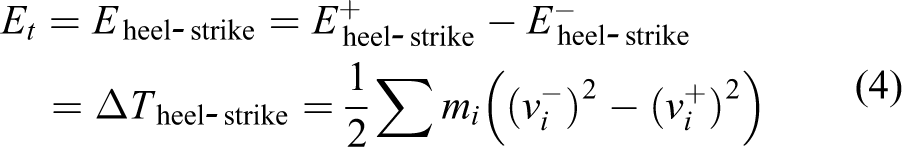
\begin{array}{l} E_{t} = E_{heel - strike} = E_{heel - strike}^{+} - E_{heel - strike}^{-} \\ = Δ T_{heel - strike} = \frac{1}{2} \sum m_{i} ({(v_{i}^{-})}^{2} - {(v_{i}^{+})}^{2}) \end{array}

where m_i is the mass points of the model; $v_{i}^{+}$ and $v_{i}^{-}$ are the velocities of the mass points just after and before the heel-strike, respectively.

The energy cost of the push-off E _push-off can be calculated by the kinetic energy difference ΔT_push-off

E_{push - off} = Δ T_{push - off} = \frac{1}{2} \sum m_{i} ({(v_{p i}^{+})}^{2} - {(v_{p i}^{-})}^{2})

where $v_{p i}^{+}$ and $v_{p i}^{-}$ are the velocities of the mass points just after and before the push-off, respectively.

Since the heel-strike impact is applied just after the push-off impact, we can get the velocity relation $v_{i}^{-} = v_{p i}^{+}$ . Therefore, from equations (3), (4), and (5), the energy cost during the swing phase E _swing is obtained

E_{swing} = Δ T_{swing} = \frac{1}{2} \sum m_{i} ({(v_{p i}^{-})}^{2} - {(v_{i}^{+})}^{2})

Energy-optimal control problem

With certain of predetermined gait constraints, such as walking speed and step length, there are infinite gait trajectories, including different initial joint velocities and actuation strategies. Our optimization goal is to find the walking gait trajectory with minimal COT by free search among these numbers of possible solutions. This can be described as a constrained nonlinear problem that minimizing the walking COT subject to the functional constraints.

Variables of the walking gait

The gait trajectory consists of the initial conditions of the walking motion, the hip torque as a function of time, and the push-off impulse. The walking gait can be described using this set of variables.

The initial conditions of the periodic walking gait include the initial angle of the two legs and their angular velocities

q (t = 0) = {(q_{1}, q_{2}, {\dot{q}}_{1}, {\dot{q}}_{2})}^{T}

The hip joint torque, which is a function of time t, determines the walking trajectory during the swing phase. However, if the joint torque is continuous time, this nonlinear optimal control problem is infinite dimensional. Therefore, we use a numerical approach to create a finite number of variables by discretizing the swing phase into N parts with the same interval. The periodic time t _step is divided into N parts t₀, t₁, …, t_N, where the interval duration $d = t_{i + 1} - t_{i} = t_{step} / N, i = 0, 1, \dots, N, t_{0} = 0, t_{N} = t_{step}$ .

Here, the joint torques are approximated by the continuous cubic spline interpolation with the N + 1 variable $τ (t = t_{0}), τ (t = t_{1}), \dots, τ (t = t_{N})$ on the grid points.

The impulse force p_psh at the push-off is also defined as the variable of the walking gait.

Functional constraints

The constraints of the walking gait include the physical system and the predetermined parameters of the walking speed and the step length. In the optimization process, minimum number of constraints is considered for finding the optimal solution in a wide range of variables.

The reasonable boundaries are enforced on the walking variables

{\begin{cases} | q_{1} | \leq π / 2, | q_{2} | \leq π \\ | {\dot{q}}_{1} | \leq u_{max}, | {\dot{q}}_{2} | \leq u_{max} \\ | τ_{hip} | \leq τ_{max} \\ 0 \leq p_{psh} \leq p_{max} \\ t_{step} \geq 0 \end{cases}

The physical constraints are designed to ensure the motion, which is a periodic walking gait (equation (9)). The periodic motion requires that the initial conditions at the beginning of the walking cycle q(t = 0) must be identical with the next step; the time that the swing leg contacts with the ground is at the heel-strike (t = t_step); all mass points of the model must be above the ground; the velocity of the swing foot along the y-axis just before the heel-strike must be smaller than zero, which ensures that the swing foot lands from above; and the normal force u_N at the stance foot should be bigger than zero to satisfy the physical constraint of walking

{\begin{cases} q (t = 0) = q_{h}^{+} (t =) t_{step} \\ 2 q_{1} (t = t_{step}) = - q_{2} (t = t_{step}) \\ y_{mass points} \geq 0 \\ {\dot{y}}_{swing foot} (t = t_{step}) < 0 \\ u_{N} \geq 0 \end{cases}

The predetermined walking speed V and step length D are specified to constrain the walking motion

{\begin{cases} v_{step} = V \\ d_{step} = D \end{cases}

Optimization process

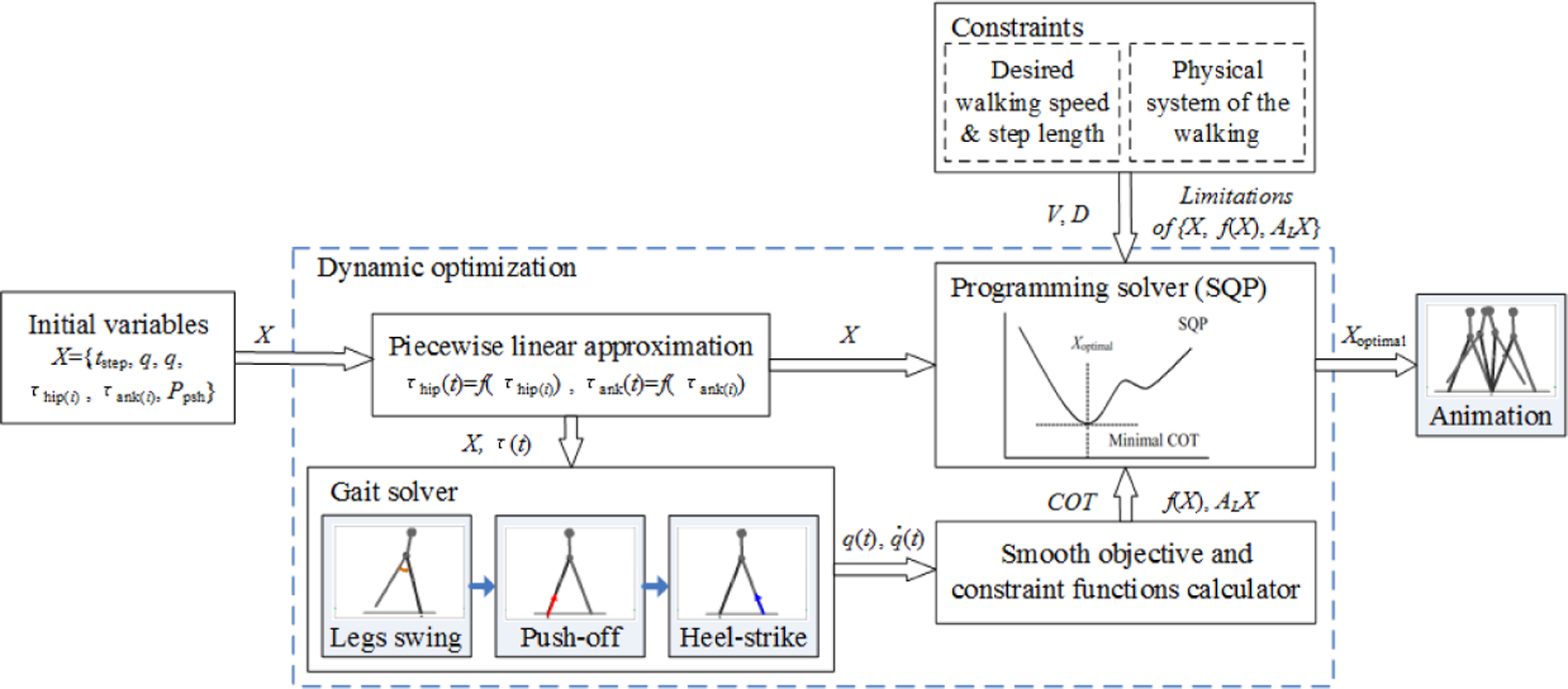
The optimization process is shown in Figure 3. The inputs of the system are the initial variables of the model X and the constraints, including the physical constraints and the desired walking speed V and step length D. The output of the system is the optimal walking gait. The continuous hip joint torque τ(t) is obtained by cubic spline interpolation of the torque variables on the grid points. With the initial variables and the continuous hip joint torque, the walking gait is calculated by the Gait Solver. The equations of motion are integrated till the end of the swing phase (t = t _step). Then, the instantaneous push-off and the heel-strike events are applied subsequently. For each integration of a full step, the COT and the constraint functions are calculated by the smooth objective and constraint functions calculator. The optimization problem is solved by the programming solver using the sequential quadratic programming package SNOPT,³⁴ with the inputs of the initial variables X, the objective function COT, and the constraints. The variables are varied to minimize the energy cost of the walking motion while respecting the constraints. Finally, the energy-optimal walking gait is obtained.

Figure 3.

Dynamic optimization control system.

Results and discussions

Model parameters study

The energy efficiency of the walking is influenced by the upper body parameters of the model. Here, we will study the effects of the length and mass parameters of the upper body on the walking efficiency. The optimal gaits with minimum COT are calculated with the parameters from Table 1. The influence of the variation of the grid points number N on the optimal results has been checked. It shows that the minimum COT is slightly decreasing with the increase of N, but the overall behavior of the optimal results does not change.

Since the qualitative results are not highly sensitive to the model parameter values,¹⁹ the COT of the optimal walking gaits is calculated with R_m = 0.7 which is from a rough estimation of human proportions. Figure 4 shows the relations of the COT and the parameters, including the upper body length l_b , the step length D, and the walking speed V. The small window in each subfigure with a certain walking speed shows the sectional view of the COT versus l_b and D. We can see that with the increase of walking speed, more energy will be cost when walking with short step length than long step length. When the upper body length and walking speed are fixed, the COT is increasing and then decreasing with the increase of the step length. It indicates that with fixed upper body length, there will be a corresponding step length for various walking speed to make the walking gait most efficient. We can also find that with the increase of the upper body length, the COT is increasing when walking with short step length, while the COT is decreasing and then getting almost flat when walking with long step length. It shows that for a set of walking speed and step length, there is a corresponding upper body length for walking with minimal COT. For the medium size of step length (D_m ∈ [0.6, 0.8]), the COT curve is almost flat with the increase of the upper body length, which indicates that the effect of l_b on the COT is not obvious when walking within this range of step length D_m .

Figure 4.

COT of the optimal walking gaits versus the upper body length l_b and step length D with different walking speeds V∈[0.3, 0.8].

Different upper body lengths will lead to different walking efficiencies. With different combinations of walking speed and step length, the corresponding upper body length l_b for walking with minimal COT is shown in Figure 5. For short step length, walking gait is the most efficient when the upper body length is zero which means that the upper body mass point is at the hip. However, for the step length bigger than 0.5, the corresponding upper body length for the walking with minimal COT is not zero, and it is increasing with the increase of the step length. For example, walking with V = 0.3 and D = 0.7, the COT = 0.19 is minimal when setting the upper body length l_b =0.2. We can also see that the value of the corresponding upper body length is maximal when walking with slow speed and long step length. Compared with the step length, the corresponding upper body length is not very sensitive to the walking speed.

Figure 5.

Corresponding upper body length l_b for the walking gaits with minimal COT.

Figure 6 shows the relations between the upper body length and the average COT of the walking within the range of walking speed and step length in Table 1. The average COT is calculated by

{COT}_{ave} = \frac{\sum_{v = v_{min}}^{v_{max}} \sum_{d = d_{min}}^{d_{max}} {COT}_{vd}}{v_{n} d_{n}}

where v_n and d_n are the numbers of the interval duration in the range of walking speed and step length. The COT_vd is the COT at the grid point with a certain combination of v and d.

Figure 6.

Average COT of the walking versus the upper body length.

It shows that the COT_ave is decreasing and then increasing with the increase of the upper body length. The minimal value of the COT_ave = 0.655 is at l_b = 0.17. It indicates that with the model parameters from Table 1, this value of upper body length is the best solution to improve the walking efficiency.

With the increase of the walking speed, the minimal normal force N _min at the stance foot during the whole walking process will decrease from a positive value to zero. Figure 7 shows the corresponding regions of N _min > 0 and N _min = 0 divided by the curve of each upper body length l_b . For example, with l_b = 0.2 and D = 0.3, if the walking speed V < 0.69, the minimal normal force N _min is bigger than zero, otherwise N _min equals zero. The region of N _min > 0 indicates that the walking gait in this region is reasonable, while the region of N _min = 0 indicates that there may be some other kinds of gait, like running, which is more efficient than walking in this region. We can find that with the increase of the upper body length l_b , the region of N _min > 0 is getting larger, and walking gait is still the optimal gait for higher speed.

Figure 7.

Regions of the minimal normal force N _min at the stance foot calculated with different upper body lengths l_b .

The effects of the upper body mass on the walking efficiency will be studied with the fixed upper body length l_b = 0.2, which is set according to the analysis results of the upper body length above. Figure 8 shows the relationship between the COT of the optimal walking gaits and the upper body mass parameter R_m with the walking speeds V = 0.4 and V = 0.6, respectively. With the increase of R_m , the COT is increasing for short step length, while the COT is decreasing for long step length. When D = 0.7 which is the middle value in the range of the step length, the COT is almost constant. It indicates that the short step length walking is more efficient with lighter upper body mass and vice versa. We cannot find an optimal solution of the upper body mass for the minimal average COT of the walking with a range of walking speed and step length. The regions of the minimal normal force during the walking N _min > 0 and N _min = 0 are shown in Figure 9, which indicates that the region of walking gait is getting larger with the increase of the upper body mass.

Figure 8.

COT of the optimal walking gaits versus the upper body mass parameter R_m (ratio of m_b and m _hb): (a) V = 0.4; (b) V = 0.6.

Figure 9.

Regions of the minimal normal force N _min at the stance foot calculated with different upper body mass parameters R_m .

Optimal gait features

The features of the optimal gaits with minimal COT are studied using the mass and length distribution parameters, l_b = 0.2 and m_b = 0.7, which are chosen from our study in “Model parameters study” section.

Figure 10 shows the comparison of the inverted pendulum walking model¹⁰ and our model. When the step length D = 1.0, the two results are almost the same. The COT is increasing with the increase of walking speed. When D = 0.5, with the increase of walking speed, the difference of the two results is getting large. The difference of the two models is that Srinivasan’s inverted pendulum model has no leg mass, and the energy for swinging the leg during the walking is not considered. In our calculation, for long step length (D = 1.0), the energy cost at push-off COT_push-off takes most proportion in the total COT, while the energy cost during walking process COT_swing takes little proportion. This is the reason that the two results are almost the same for long step length. For short step length (D = 0.5), the COT_swing takes more proportion with the increase of walking speed. It explains that the difference between the results of the two models.

Figure 10.

Comparison of the inverted pendulum walking model (Srinivasan) and our calculation.

Figure 11 shows the gaits features of the walking motion with a range of walking speed and step length. From the relation of the COT and the step length (Figure 11(a)), we can see that the COT curve is a quadratic with minimal value with the increase of the step length, which indicates that for a certain walking speed, the optimal walking gait can be found with a corresponding step length. The relation of the COT and the walking speed shows that the COT is increasing with the increase of the walking speed.

Figure 11.

Walking gait features with a range of step length and speed (l_b = 0.2 and R_m = 0.7): (a) COT of the walking gait; (b) push-off impulse P _psh; (c) minimal normal force N _min.

The push-off impulse of the walking is increasing with the increase of the walking speed and the step length (Figure 11(b)). Since the push-off impulse is proportional to the COT_push-off, with the increase of the walking speed and the step length, the COT_push-off is increasing. Figure 11(c) shows that the minimal normal force during the walking N _min is increasing with the increase of the walking speed. For slow walking speed, N _min is decreasing with the increase of the step length, but when V = 0.6, the curve of N _min is almost flat. It indicates that with the increase of the walking speed, the minimal normal force during the waking is less sensitive to the step length.

In our calculation, we find that although the quantitative results of the walking gaits within a range of walking speed and step length are different, the qualitative results of these walking gaits are similar. Therefore, the stick figure and features of the typical walking gait with the walking speed V = 0.5 and the step length D = 1.0 are shown in Figure 12. We find that the upper body slightly rotates forward and then backward during a walking step. The stance leg swings like an inverted pendulum with a speed which is decreasing and then increasing. The swing leg rotates forward with a speed which is increasing and then decreasing.

Figure 12.

Stick figure and features of the walking gait (V = 0.5 and D = 1.0).

During the swing phase, the hip joint torque is the only actuator. The typical strategy of the optimal walking gait is that the hip joint torque is just at the beginning of the step.^13,16 For the gird point number N = 10, the hip joint torque is bigger than 0 before t < 0.2 (1/N). If N is changed, the hip joint torque is still at the first interval duration, and the area under the hip torque, which determines the energy cost during the swing phase COT_swing, is unchanged.

Conclusion

This article studies the effects of the upper body parameters, including upper body length and mass, on the walking efficiency using a dynamic optimization method. For a combination of walking speed and step length, there is a corresponding upper body length for walking with minimal COT. If the step length is short, walking gait is the most efficient when the upper body length is zero, which means that the upper body mass point is at the hip. If the step length is bigger than 0.5, the corresponding upper body length is not zero and increases with the increase of the step length. Compared with the step length, the corresponding upper body length is not very sensitive to the walking speed. The minimal average COT is calculated with the upper body length l_b = 0.17, which is the optimal solution for the efficient walking. We also find that the short step length walking is more efficient with lighter upper body mass and vice versa. There is no optimal solution of the upper body mass for the minimal average COT of the walking with a range of walking speed and step length.

By calculating the minimal normal force N _min at the stance foot during the walking process, we find that with the increase of the upper body length and mass, the region of N _min > 0 is getting larger, and walking gait is still the optimal gait for higher speed than other kind of gaits that the stance foot is not on the ground.

We also present the features of the optimal walking gaits with the combinations of walking speed and step length. The typical strategy of the optimal walking gait is that the hip joint torque is just at the beginning of the step.

These studies can not only help us to understand the mechanism of the energetic walking but also provide suggestions for designing upper body for advanced legged robots with high energy efficiency. For example, mechanical parameters improvement and efficient control strategy design.

Footnotes

Declaration of conflicting interests

The author(s) declared no potential conflicts of interest with respect to the research, authorship, and/or publication of this article.

Funding

The author(s) disclosed receipt of the following financial support for the research, authorship, and/or publication of this article: This work was supported by the National Natural Science Foundation of China (grant no. 61673300), the Shanghai Natural Science Foundation (grant no. 16ZR1424600), the research project of the Science and Technology Commission of Shanghai Municipality (grant no. 16070502900), the University’s Scientific Research Project (grant no. SK201511), the Training Program Foundation for Shanghai Young University Teacher (grant no. ZZssd15054), and the Chongqing Basic Science and Advanced Technology Research Project (grant no. cstc2015jcyjA40041).

Appendix 1

References

Kuindersma

Deits

Fallon

. Optimization-based locomotion planning, estimation, and control design for the Atlas humanoid robot. Auton Robot 2016; 40(3): 429–455.

DRC-HUBO. http://www.drc-hubo.com/ (accessed 5 June 2015).

DARPA Robotics Challenge (DRC) Finals 2015. http://www.theroboticschallenge.org/ (accessed 5 June 2015).

McGeer

. Passive dynamic walking. Int J Robot Res 1990; 9: 68–82.

Goswami

Thuilot

Espiau

Compass-like biped robot part I: Stability and bifurcation of passive gaits. Technical Report. INRIA, France, 1996.

Goswami

Espiau

Keramane

. Limit cycles in a passive compass gait biped and passivity-mimicking control laws. Auton Robot 1997; 4(3): 273–286.

Goswami

Thuilot

Espiau

. A study of the passive gait of a compass-like biped robot: symmetry and chaos. Int J Rob Res 1998; 17(12): 1282–1301.

Garcia

Chatterjee

Ruina

. Simplest walking model: stability, complexity, and scaling. J Biomech Eng Trans ASME 1998; 120(2): 281–288.

Garcia

Chatterjee

Ruina

. Efficiency, speed, and scaling of passive dynamic walking. Dyn Stab Syst 2000; 15: 75–99.

10.

Srinivasan

Ruina

. Computer optimization of a minimal biped model discovers walking and running. Nature 2006; 439: 72–75.

11.

Srinivasan

Ruina

. Idealized walking and running gaits minimize work. Proc R Soc Lond A Math Phys Sci 2007; 463: 2429–2446.

12.

Srinivasan

. Fifteen observations on the structure of energy-minimizing gaits in many simple biped models. J R Soc Interface 2011; 8: 74–98.

13.

Hasaneini

Macnab

CJB

Bertram

JEA

. The dynamic optimization approach to locomotion dynamics: human-like gaits from a minimally constrained biped model. Advanced Robotics. 2013; 27(11): 845–859

14.

Hasaneini

Macnab

CJB

Bertram

JEA

. Dynamic optimization clearly shows the determinants of bipedal gaits: reduced gravity predictions and verification. In: Dynamic walking, Florida, USA, 21 5 2012.

15.

Collins

Ruina

Tedrake

. Efficient bipedal robots based on passive dynamic walkers. Sci Mag 2005; 307: 1082–1085.

16.

Bhounsule

Cortell

Grewal

. Low-bandwidth reflex-based control for lower power walking: 65 km on a single battery charge. Int J Robot Res 2014; 33(10): 1305–1321.

17.

Sreenath

Park

Poulakakis

. Embedding active force control within the compliant hybrid zero dynamics to achieve stable, fast running on MABEL. Int J Robot Res 2014; 33: 988–1005.

18.

Ramezani

Hurst

JW,

Hamed

. Performance analysis and feedback control of ATRIAS, a three-dimensional bipedal robot. J Dyn Syst Meas Control 2013; 136(2): 021012.

19.

Kang

Qijun

. Dynamic optimization of a biped model: energetic walking gaits with different mechanical and gait parameters. Adv Mech Eng 2015; 7(5): 1–13.

20.

Wisse

Schwab

AL,

van der Helm

FCT

. Passive dynamic walking model with upper body. Robotica 2004; 22: 681–688.

21.

Wisse

Hobbelen

DGE,

Schwab

. Adding an upper body to passive dynamic walking robots by means of a bisecting hip mechanism. IEEE Trans Robot 2007; 23(1): 112–123.

22.

Gomes

Ruina

. Walking model with no energy cost. Phys Rev E 2011; 83(3): 032901.

23.

Chyou

Liddell

GF,

Paulin

. An upper-body can improve the stability and efficiency of passive dynamic walking. J Theor Biol 2011; 285: 126–135.

24.

Honjo

Nagano

Luo

. Parametrically excited inverted double pendulum and efficient bipedal walking with an upper body. Robotica 2013; 31(6): 875–886.

25.

Guo

JL,

Yang

. Bifurcation and chaos in the simple passive dynamic walking model with upper body. Chaos 2014; 24: 033114.

26.

Kuo

. A simple model of bipedal walking predicts the preferred speed–step length relationship. J Biomech Eng 2001; 123: 264–269.

27.

Kuo

. Energetics of actively powered locomotion using the simplest walking model. J Biomech Eng 2002; 124: 113–120.

28.

Yamakita

Asano

. Extended passive velocity field control with variable velocity fields for a kneed biped. Adv Robot 2001; 15(2): 139–168.

29.

Naval Biodynamics Laboratory. Anthropometry and mass distribution for human analogues. Volume I: Military Male Aviators. USAARL Report. Fort Rucker: USAARL, 1988.

30.

Winter

. Biomechanics and motor control of human movement. New Jersey: John Wiley & Sons, 2005.

31.

Schwab

Wisse

Basin of attraction of the simplest walking model. In: Proceedings of the ASME design engineering technical conference, Pittsburgh, PA, 9 September 2001, pp. 531–539, ASME.

32.

Ruina

Bertram

JEA,

Srinivasan

. A collisional model of the energetic cost of support work qualitatively explains leg sequencing in walking and galloping, pseudo-elastic leg behavior in running and the walk-to-run transition. J Theor Biol 2005; 237: 170–192.

33.

Adamczyk

Kuo

. Redirection of center-of-mass velocity during the step-to-step transition of human walking. J Exp Biol 2009; 212: 2668–2678.

34.

Gill

Murray

Saunders

MA. SNOPT

: An SQP algorithm for large-scale constrained optimization (Reprinted from SIAM Journal Optimization, 2002, 12: 979-1006). SIAM Rev 2005; 47(1): 99–131.

Effects of upper body parameters on biped walking efficiency studied by dynamic optimization

Abstract

Keywords

Introduction

Analysis of the walking motion

Analysis of the model

The walking motion

Cost function of the walking

Energy-optimal control problem

Variables of the walking gait

Functional constraints

Optimization process

Results and discussions

Model parameters study

Optimal gait features

Conclusion

Footnotes

Declaration of conflicting interests

Funding

Appendix 1

References