Dynamic optimization of a biped model: Energetic walking gaits with different mechanical and gait parameters

Abstract

Energy consumption is one of the problems for bipedal robots walking. For the purpose of studying the parameter effects on the design of energetic walking bipeds with strong adaptability, we use a dynamic optimization method on our new walking model to first investigate the effects of the mechanical parameters, including mass and length distribution, on the walking efficiency. Then, we study the energetic walking gait features with the combinations of walking speed and step length. Our walking model is designed upon Srinivasan’s model. Dynamic optimization is used for a free search with minimal constraints. The results show that the cost of transport of a certain gait increases with the increase in the mass and length distribution parameters, except for that the cost of transport decreases with big length distribution parameter and long step length. We can also find a corresponding range of walking speed and step length, in which the variation in one of the two parameters has no obvious effect on the cost of transport. With fixed mechanical parameters, the cost of transport increases with the increase in the walking speed. There is a speed–step length relationship for walking with minimal cost of transport. The hip torque output strategy is adjusted in two situations to meet the walking requirements.

Introduction

In the recent years, the area of bipedal robot has been paid more attention. Some institutes have successfully built their excellent walking bipeds which can walk with various gaits, such as different walking speed and step length, to adapt to various walking situations. However, one problem for the walking task is energy consumption. For example, Boston Dynamics developed the biped robots, PETMAN ¹ and Atlas, ² which can balance themselves and walk freely with natural agile gait, but the cost of transport (COT) of the robots is about 5 ³ which is about 15 times than that of a walking person.

An effective solution for energetic efficiency is the exploitation of the “natural dynamics” of the walking system. ⁴ Since McGeer ⁵ first introduced the passive dynamic walking that an unactuated and uncontrolled biped machine can walk stably on a shallow slope, Goswami and Garcia deeply studied the simple walking model. They presented two well-known walking models, the compass-like biped model^6–8 and the simplest walking model,^9,10 respectively, and discussed the relation between model parameters and gaits. Then, some researchers used human data and experience model to study the walking mechanism. Kuo analyzed the mechanical work in the transition between steps^11,12 and presented the method to obtain energy by improving the economy of the walking. ¹³ Donelan found the relation between energy cost and walking parameters, such as frequency, step length, and step width.^14,15 Doke et al. ¹⁶ measured the metabolic energy expended to swing a human leg. After that, some researchers studied the walking dynamics using optimization methods. Srinivasan presented a point-mass legged model. Using energy-optimal trajectory control, he showed that people mostly use walk at low speeds and run at fast speeds, and at intermediate speeds a new kind of walk is discovered, which is called pendular-run.^17–19 Hasaneini et al.^20,21 presented a simple biped model with an optimization approach for the locomotion dynamics. By several years study on the mechanism of walking, some energetic bipedal robots with high energy efficiency have been designed. ²² Ruina built the robot Ranger which walks 60 km non-stop with little energy cost.^4,23–25 Grizzle and colleagues ²⁶ made the robot MARLO which does not need a boom for support and has on-board power. Karssen and Wisse designed the robot Phides which has a human-like morphology and gait. ²⁷ Most of these researches, however, mainly focused on studying the walking gait features to understand the mechanism of walking.

Walking robots with different mechanical parameters, such as mass and length distribution, have different walking performance.^28–31 This leads us to believe that for designing energy-optimal walking robot, the optimization of mechanical parameters is also as important as the study of walking gait features. Furthermore, the two gait parameters, including walking speed and step length, are commonly used to determine various gaits.^12,17 Although Srinivasan and Ruina ¹⁷ and Hasaneini et al. ²⁰ studied the energetic walking motion with some parameters, such as walking speed and slope angle, there is still a need for an elaborate investigation on the energetic walking motion with the combinations of walking speed and step length for the purpose of understanding the energetic walking gait features under various walking situations. Therefore, in this article, we use a dynamic optimization method on our new walking model to first investigate the effects of the mechanical parameters, including mass and length distribution, on the walking efficiency. Then, we study the energetic walking gait features with the combinations of walking speed and step length.

Our walking model is designed upon Srinivasan’s model which equivalently includes a mass point on hip, massless legs, and only one actuation push-off impulse. ¹⁷ We add adjustable mass points on the two fixed-length legs for studying the effects of the mass and length distribution on the walking efficiency. Hip torque, which is another typical actuation design for building walking robot besides the push-off impulse, ³² is added on the model for actuating the swing leg during the walking process. Since simple models can lead to powerful insights regarding the dynamics of complex walking and its associated energetic gait features, ³³ compared with Hasaneini’s more complex model, ²⁰ our model is more suitable for the purpose of this article.

Dynamic optimization method is used to search the energetic walking gaits with walking constraints. The optimal solution is searched freely among a wide range of possible solutions with minimal constraints which just include the physical walking system and the desired parameters such as the walking speed and the step length.

Analysis of the walking motion

A three mass points and two sticks biped model is used to study the walking motion. Three mass points are at the hip m_h on the legs m _l (Figure 1). The leg with a point foot on the ground is labeled as stance leg and the leg without a foot on the ground is labeled as swing leg. In the walking process, two actuators are used: rotational joint torque at the hip τ_hip and instantaneous push-off impulse at the stance foot P_psh .

Figure 1.

A typical step of the walking model: (a) initial conditions, (b) swing phase, (c) instantaneous push-off, and (d) instantaneous heel-strike.

The walking motion

The periodic walking motion includes three parts: swing phase, instantaneous push-off process, and heel-strike process. The swing phase begins at the instant that the two legs are both on the level ground, just after the stance foot hit the slope at heel-strike and the swing foot is away from the ground. Before the instant that the swing foot makes contact with the ground, the swing phase ends. Then, the push-off process is applied instantaneously between the end of the swing phase and the heel-strike process which sets the initial conditions for the following step.

Here, we assume that the collision at heel-strike is a no-bounce process and there is no double support after heel-strike. The instantaneous push-off just before heel-strike is a strategy to reduce the collision loss, which is a classical design for the energy-optimal walking motion.^34,35 For simplicity, we assume that the model has two massless point feet which are equivalent to massless flat feet that are parallel to the ground surface. ²⁰ We also assume that there is sufficient friction between the feet and the ground surface to prevent slippage during the whole walking process.

During the swing process, the swing foot is briefly below the ground level when the stance leg is near vertical which explains the inevitable scuffing problem of some straight-legged walkers. ¹⁰ Therefore, we allow the briefly swing foot scuffing in midstance during the swing phase. In physical models, knees, three-dimensional (3D) motion, or leg shortening measures can solve the problem, but the complexity of the model will increase. ⁵

Analysis of the model

The walking model includes two legs that are hinged at the hip. The leg length is l and the mass point on the leg is located at the point that the distance to the hip is l_t . q ₁ is the angle of the stance leg with respect to the ground surface normal. q ₂ is the angle between the swing leg and the stance leg, where the counterclockwise angle is positive. (x ₀, y ₀) defines the coordinates of the stance foot in the rectangular coordinate system that the forward and upward directions are positive and the initial position of the stance foot is (0, 0). Therefore, the walking model can be described by the generalized coordinates $q={(q_1,q_2,x_0,y_0)}^T$ which characterize 4 degrees of freedom (DOFs) of the model.

Our walking model includes not only the generalized coordinates q ₁, q ₂ that describe the status of the two legs but also the generalized coordinates of the stance foot x ₀, y ₀. There are two advantages: (1) during the swing phase, the stance foot is the only point that contact with the ground. The constrained forces of the stance foot that include the normal force and the friction force can be obtained by constraining the position of the stance foot. Therefore, the friction force, and whether the stance foot leaves the ground can be checked to meet the walking constraints. (2) The instantaneous processes push-off and heel-strike can be described by the equivalent impulses that contact with the ground. The conventional angular momentum conservation ³⁶ is not needed for solving the heel-strike process.

Cost function of the walking

The energy cost per unit distance traveled ⁴ is used as the objective function for finding the optimal gait that minimizes the energy cost subject to physical constraints.

The energy cost of one step of the walking E_t is expressed by

$$E_t=E_{\mathrm{swing}}+E_{\mathrm{push}-\mathrm{off}}$$

(1)

where E_swing is the energy cost during the swing phase and E_push-off is the energy cost of push-off process.

These two energy cost items are described as follows

$$\{\begin{array}{c}\hfill E_{\mathrm{swing}}=\underset{0}{\overset{t}{\int }}\left|P_{\mathrm{hip}}\right|\mathrm{dt}\hfill \\ \multicolumn{1}{c}{E_{\mathrm{push}-\mathrm{off}}=E_{\mathrm{push}-\mathrm{off}}^{+}-E_{\mathrm{push}-\mathrm{off}}^{-}}\end{array}$$

(2)

where t is the periodic time of one step and P_hip is the mechanical power of the hip joint torque. $E_{\mathrm{push}-\mathrm{off}}^{+}$ and $E_{\mathrm{push}-\mathrm{off}}^{-}$ are the mechanical energy of the model just after and before the push-off process, respectively. Since the potential energy is constant, $E_{\mathrm{push}-\mathrm{off}}$ could be expressed by the kinetic energy difference between the moment just after and before push-off $\Delta T_{\mathrm{push}-\mathrm{off}}$

$$\{\begin{array}{c}\hfill P_{\mathrm{hip}}={\stackrel{·}{q}}_2{\tau }_{\mathrm{hip}}\hfill \\ \multicolumn{1}{c}{E_{\mathrm{push}-\mathrm{off}}=\Delta T_{\mathrm{push}-\mathrm{off}}=\frac{1}{2}\sum m_i({(v_i^{+})}^2-{(v_i^{-})}^2)}\end{array}$$

(3)

The COT that is defined as the total energy cost of the walking per distance traveled and per unit body weight can be estimated as

$$\begin{array}{cc}\multicolumn{1}{c}{\mathrm{COT}}& =\frac{\mathrm{Energy}\mathrm{per}\mathrm{step}}{\mathrm{Weight}\times \mathrm{Step}\mathrm{Length}}=\frac{E_t}{m_{\mathrm{total}}\mathrm{gD}}\hfill \\ \multicolumn{1}{c}{}& ={\mathrm{COT}}_{\mathrm{push}-\mathrm{off}}+{\mathrm{COT}}_{\mathrm{swing}}\hfill \end{array}$$

(4)

where $m_{\mathrm{total}}$ is the total mass of the model, $D$ is the step length of the walking gait, and g is the acceleration of gravity. Therefore, the total COT of the walking includes the COT at push-off and the COT during swing phase: COT _push-off and COT _swing .

The energy input of the model is E_t , and the energy output of the model is E_heel-strike which is the energy of the collision lost at heel-strike. Since the walking gait is a periodic motion, the energy cost of one step is constant. The following equation could be obtained

$$E_t=E_{\mathrm{heel}-\mathrm{strike}}$$

(5)

Equations of motion

We use Lagrange’s equation (equation (6)) to derive the equations of motion (EoM) of the walking model

$$\{\begin{array}{c}\hfill \frac{d}{\mathrm{dt}}\left(\frac{\partial L}{\partial \stackrel{·}{q}}\right)-\frac{\partial L}{\partial q}=0\hfill \\ \multicolumn{1}{c}{L=T-V}\end{array}$$

(6)

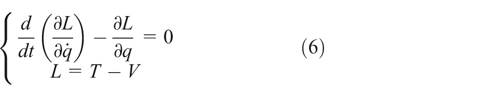
where Lagrangian L is the difference between the kinetic energy of the system, T, and its potential energy, V.

T and V can be calculated by defining a global vector X = (x_stl , y_stl , x_hip , y_hip , x_swl , y_swl ) ^T which is the coordinates of the three mass points describing the whole configuration of the walking model. The expression of X which is a function of the generalized coordinates q = (q ₁, q ₂, x ₀, y ₀) ^T is described as follows

$$X=\left[\begin{array}{c}\hfill x_{\mathrm{stl}}\hfill \\ \multicolumn{1}{c}{y_{\mathrm{stl}}}\\ \multicolumn{1}{c}{\begin{array}{c}\hfill \begin{array}{c}\hfill x_{\mathrm{hip}}\hfill \\ \multicolumn{1}{c}{y_{\mathrm{hip}}}\end{array}\hfill \\ \multicolumn{1}{c}{x_{\mathrm{swl}}}\end{array}}\\ \multicolumn{1}{c}{y_{\mathrm{swl}}}\end{array}\right]=\left[\begin{array}{c}\hfill x_0-l_s\sin (q_1)\hfill \\ \multicolumn{1}{c}{y_0+l_s\cos (q_1)}\\ \multicolumn{1}{c}{\begin{array}{c}\hfill \begin{array}{c}\hfill x_0-(l_s+l_t)\sin (q_1)\hfill \\ \multicolumn{1}{c}{y_0+(l_s+l_t)\cos (q_1)}\end{array}\hfill \\ \multicolumn{1}{c}{x_0-(l_s+l_t)\sin (q_1)+l_t\sin (q_1+q_2)}\end{array}}\\ \multicolumn{1}{c}{y_0+(l_s+l_t)\cos (q_1)-l_t\cos (q_1+q_2)}\end{array}\right]$$

(7)

These equations above yield the EoM of the swing phase

$$M(q)\stackrel{··}{q}+C(q,\stackrel{·}{q})\stackrel{·}{q}+G(q,\gamma )=J_r^{T}u+T$$

(8)

where $M(q)$ is a 4 × 4 matrix, $C(q,\stackrel{·}{q})\stackrel{·}{q}$ and $G(q,\gamma )$ are 4 × 1 matrices, $J_r^{T}u$ is the constrained force at the stance foot (described below in section “Constrained force at stance foot”), $T=[0{\tau }_{\mathrm{hip}}00{]}^T$ , and $\gamma$ is the angle of slope. Here, $\gamma =0$ .

Constrained force at stance foot

In our walking model, there are two DOFs at the stance foot. The constrained force at stance foot is designed to keep the position of the stance foot constant to meet the physical constraints: no slippage between the stance foot and the ground which is constrained by the forward force that is parallel to the ground, and the stance foot is above the ground surface which is constrained by the upward force that is vertical to the ground. The constrained condition at the stance foot is

$$J_r[\begin{array}{ccc}\hfill q\hfill & \hfill \stackrel{·}{q}\hfill & \hfill \stackrel{··}{q}\hfill \end{array}]=0,J_r=\left[\begin{array}{c}\hfill \begin{array}{cccc}\hfill 0\hfill & \hfill 0\hfill & \hfill 1\hfill & \hfill 0\hfill \end{array}\hfill \\ \multicolumn{1}{c}{\begin{array}{cccc}\hfill 0\hfill & \hfill 0\hfill & \hfill 0\hfill & \hfill 1\hfill \end{array}}\end{array}\right]$$

(9)

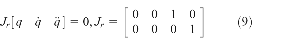
where the generalized coordinate q is 4 × 1 matrices.

From equations (8) and (9), we obtain the following relation

$$J_r\stackrel{··}{q}=-J_{r}M{(q)}^{-1}(C(q,\stackrel{·}{q})\stackrel{·}{q}+G(q,\gamma )-J_r^{T}u-T)=0$$

(10)

Therefore, the constrained force at the stance foot $u=[\begin{array}{cc}\hfill u_F\hfill & \hfill u_N\hfill \end{array}{]}^T$ is obtained as follows, where $u_F$ is the friction force and $u_N$ is the normal force

$$u={\left(J_{r}M{(q)}^{-1}{J}_r^T\right)}^{-1}{J}_{r}M{(q)}^{-1}(C(q,\stackrel{·}{q})\stackrel{·}{q}+G(q,\gamma )-T)$$

(11)

The swing phase of the walking motion can be expressed by putting functions (9) and (11) into equation (8).

Heel-strike

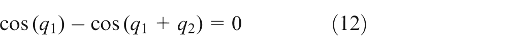
The swing foot makes contact with the ground at the heel-strike which is the end of the periodic walking motion. The angle position of the joints is constant, but the angular velocity varies discretely at the heel-strike. The geometric collision condition is

$$\cos (q_1)-\cos (q_1+q_2)=0$$

(12)

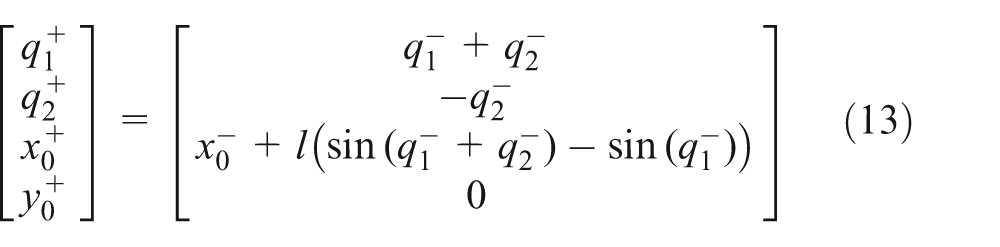
A new step begins just after the heel-strike with the initial conditions that converted from the condition just before the heel-strike. The angle position relation is given below, where the “+”means “just after the impact,” and the “−” means “just before the impact”

$$\left[\begin{array}{c}\hfill q_1^{+}\hfill \\ \multicolumn{1}{c}{q_2^{+}}\\ \multicolumn{1}{c}{x_0^{+}}\\ \multicolumn{1}{c}{y_0^{+}}\end{array}\right]=\left[\begin{array}{c}\hfill q_1^{-}+q_2^{-}\hfill \\ \multicolumn{1}{c}{-q_2^{-}}\\ \multicolumn{1}{c}{x_0^{-}+l(\sin (q_1^{-}+q_2^{-})-\sin (q_1^{-}))}\\ \multicolumn{1}{c}{0}\end{array}\right]$$

(13)

Here, we calculate the instantaneous angular velocity just after heel-strike by an equivalent impulse method which is an easier way for solving this discrete process in the robot dynamic systems than the angular momentum conservation method.

The swing foot contacts with the ground with a certain linear velocity. After the collision, since no-bounce is assumed, the swing leg switches to be the stance leg, and the velocity of the new stance foot is 0. Therefore, the equivalent impulse method is described as follows: before the heel-strike, the two legs switch their roles. The new stance foot which is the old swing leg with linear velocity will contact with the ground. And the new swing leg will leave the ground. The collision between the new stance foot and the ground is equivalent to that an instantaneous impulse force pushes the leg along the leg axis. The velocity of the new stance foot will instantaneously decrease from a certain value to 0 after the collision. The relation of the velocity before and after the status that the two legs switch their roles is given below, where “*” means “after the switch”

$$\left[\begin{array}{c}\hfill {\stackrel{·}{q}}_1^{*}\hfill \\ \multicolumn{1}{c}{{\stackrel{·}{q}}_2^{*}}\\ \multicolumn{1}{c}{{\stackrel{·}{x}}_0^{*}}\\ \multicolumn{1}{c}{{\stackrel{·}{y}}_0^{*}}\end{array}\right]=\left[\begin{array}{c}\hfill {\stackrel{·}{q}}_1^{-}+{\stackrel{·}{q}}_2^{-}\hfill \\ \multicolumn{1}{c}{-{\stackrel{·}{q}}_2^{-}}\\ \multicolumn{1}{c}{{\stackrel{·}{x}}_0^{-}+l({\stackrel{·}{q}}_1^{-}+{\stackrel{·}{q}}_2^{-})\cos (q_1^{-}+q_2^{-})-l{\stackrel{·}{q}}_1^{-}\cos (q_1^{-})}\\ \multicolumn{1}{c}{{\stackrel{·}{y}}_0^{-}+l({\stackrel{·}{q}}_1^{-}+{\stackrel{·}{q}}_2^{-})\sin (q_1^{-}+q_2^{-})-l{\stackrel{·}{q}}_1^{-}\sin (q_1^{-})}\end{array}\right]$$

(14)

The instantaneous impulse equal to the variation in the momentum of the model yields that

$$M(q^{+}){\stackrel{·}{q}}^{+}-M(q^{*}){\stackrel{·}{q}}^{*}=J_i^{T}P$$

(15)

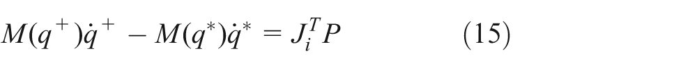
where $J_i=\left[\begin{array}{c}\hfill \begin{array}{cccc}\hfill 0\hfill & \hfill 0\hfill & \hfill 1\hfill & \hfill 0\hfill \end{array}\hfill \\ \multicolumn{1}{c}{\begin{array}{cccc}\hfill 0\hfill & \hfill 0\hfill & \hfill 0\hfill & \hfill 1\hfill \end{array}}\end{array}\right]$ ; P is a 2 × 1 matrix that expresses the instantaneous impulse forces along x- and y-axes.

After the collision, the velocity of the stance foot is 0. The following equation can be obtained

$$J_i{\stackrel{·}{q}}^{+}=0$$

(16)

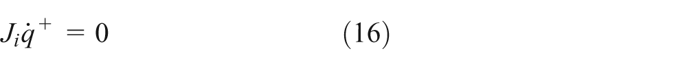
Since the switch of the two legs is before the collision, we can get $q^{+}=q^{*}$ . Equations (15) and (16) yield

$$J_i{\stackrel{·}{q}}^{*}+J_{i}M{(q^{*})}^{-1}{J}_i^{T}P=0$$

(17)

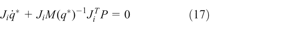
The instantaneous impulse force is derived by equation (17)

$$P=-{\left(J_{i}M{(q^{*})}^{-1}{J}_i^T\right)}^{-1}{J}_i{\stackrel{·}{q}}^{*}$$

(18)

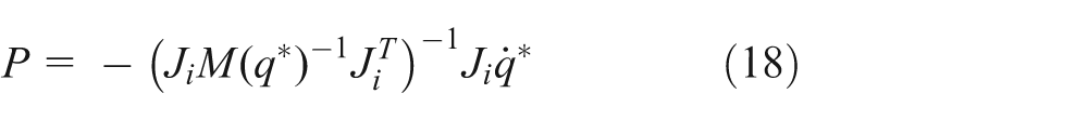
Therefore, the velocity of the model just after heel-strike is obtained by equations (15) and (18), where I is the identity matrix

$${\stackrel{·}{q}}^{+}=(I-M{(q^{*})}^{-1}{J}_i^T{\left(J_{i}M{(q^{*})}^{-1}{J}_i^T\right)}^{-1}{J}_i){\stackrel{·}{q}}^{*}$$

(19)

Push-off

The instantaneous process push-off happens just before the heel-strike, which is a design strategy to minimize the walking energy loss. ³⁷ The push-off process is considered as that an instantaneous impulse at the stance foot push the model along the stance leg axis. The amount of the impulse equals to the variation in the momentum of the model

$$M(q_p^{+}){\stackrel{·}{q}}_p^{+}-M(q_p^{+}){\stackrel{·}{q}}_p^{-}=J_p^T{P}_{\mathrm{psh}}$$

(20)

where $J_p=[\begin{array}{cccc}\hfill 0\hfill & \hfill 0\hfill & \hfill -\sin (q_1^{+})\hfill & \hfill \cos (q_1^{+})\hfill \end{array}]$ , $p_{\mathrm{psh}}$ is the impulse, and $J_p^T{P}_{\mathrm{psh}}$ is the axial component impulses of $p_{\mathrm{psh}}^x$ on x and $p_{\mathrm{psh}}^y$ on y. $q_p^{-}=[q_1^{-},q_1^{-},x_0^{-},y_0^{-}]$ and $q_p^{+}=[q_1^{+},q_1^{+},x_0^{+},y_0^{+}]$ are the conditions of the model just before and after push-off, respectively.

Therefore, the velocity just after push-off is obtained as follows

$${\stackrel{·}{q}}_p^{+}=M{(q_p^{+})}^{-1}(M(q_p^{+}){\stackrel{·}{q}}_p^{-}+J_p^T{P}_{\mathrm{psh}})$$

(21)

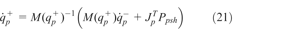
From Figure 1, we can see the velocity variations in the hip at the two instantaneous events: the push-off and the heel-strike.

Energy-optimal control problem

The energy-optimal control problem in this article is a constrained nonlinear problem which is described as that minimizing the COT of the model subject to the functional constraints (equation (22)). For giving a set of gait parameters, such as walking speed or step length, there are infinite gait trajectories that meet the predetermined requirements. Our optimal goal is to find the walking gait trajectory with minimal COT by freely searching among these numbers of possible solutions

$$\begin{array}{cc}\multicolumn{1}{c}{}& \underset{x}{\mathrm{minimize}}{f}_0(x)\hfill \\ \multicolumn{1}{c}{}& \mathrm{subject}\mathrm{to}l\le \left(\begin{array}{c}\hfill x\hfill \\ \multicolumn{1}{c}{f(x)}\\ \multicolumn{1}{c}{A_{L}x}\end{array}\right)\le u\hfill \end{array}$$

(22)

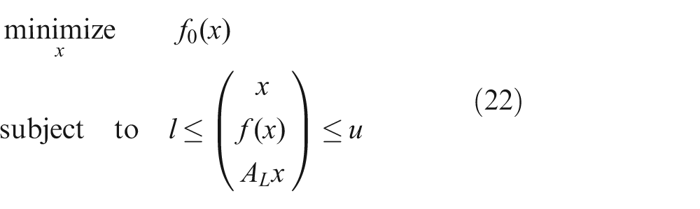
where x is an n-vector of the walking variables; l and u are constant lower and upper bounds, respectively; f ₀(x) is the smooth scalar objective function COT, A_L is a sparse matrix, and f(x) is a vector of smooth nonlinear constraint functions {f _i(x)}.

The cost function includes the absolute values (equation (2)) which cause discontinuities. This may create difficulties for solving the numerical optimization problem. Therefore, the square-root smoothing technique ³⁸ will be used in our optimization to eliminate this numerical issue.

Variables of the walking gait

The optimal solution contains a set of variables of the walking gait. By using the optimal set of variables, the model can achieve the walking gait with minimal energy cost.

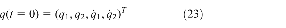
The periodic walking gait begins with the initial conditions that include the initial angle positions and velocities of the two legs

$$q(t=0)={(q_1,q_2,{\stackrel{·}{q}}_1,{\stackrel{·}{q}}_2)}^T$$

(23)

During the swing phase, the hip joint torque which is a function of time t determines the walking trajectory that starts from the initial conditions. The nonlinear optimal control problem is infinite dimensional if the variables are continuous-time. Here, we use a numerical approach to create a finite number of variables by discretizing the swing phase into N parts with the same interval. The variable t_step , which is the periodic time, is divided into N parts $t_0,t_0,\dots ,t_N$ , where the interval duration $d=t_{i+1}-t_i=1/N,i=0,1,\dots ,N,t_0=0,t_N=t_{\mathrm{step}}$ . The joint torque is approximated by the continuous piecewise linear functions with the N + 1 variables $\tau (t=t_0),\tau (t=t_1),\dots ,\tau (t=t_N)$ on the grid points.

The impulse force $p_{\mathrm{psh}}$ at the push-off just before the heel-strike is another variable of the walking gait.

Constraints

For finding the optimal solution in a wide variables’ range, minimum number of constraints is considered in our optimization process. Normally, the constraints include the physical system and the predetermined parameters such as the walking speed or step length.

For meeting the physical requirements of the walking, such as all points of the model remain above the ground, joint torque is realistic, boundaries are enforced on the walking variables

$$\{\begin{array}{c}\hfill \left|q_1\right|\le \frac{\pi }{2},\left|q_2\right|\le \pi \hfill \\ \multicolumn{1}{c}{\left|{\stackrel{·}{q}}_1\right|\le u_{\max },\left|{\stackrel{·}{q}}_2\right|\le u_{\max }}\\ \multicolumn{1}{c}{\left|{\tau }_{\mathrm{hip}}\right|\le {\tau }_{\max }}\\ \multicolumn{1}{c}{0\le p_{\mathrm{psh}}\le p_{\max }}\end{array}$$

(24)

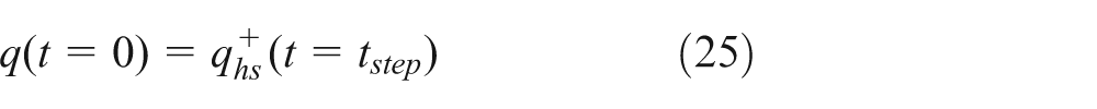
Since the walking gait is periodic, the initial conditions at the beginning of the walking cycle must be identical with the next step

$$q(t=0)=q_{\mathrm{hs}}^{+}(t=t_{\mathrm{step}})$$

(25)

The swing leg will contact with the ground at heel-strike ( $t=t_{\mathrm{step}}$ ); 2q ₁ = −q ₂ is required. The velocity of the swing foot along the y-axis just before heel-strike must be smaller than 0, which ensures that the swing foot lands from above. The normal force at stance foot should be bigger than 0 to satisfy the physical constraint of walking.

The predetermined walking speed V and the step length D can be specified to constrain the walking motion.

Optimization process

The optimization process is described as follows: with the initial conditions of the walking gait $q(t=t_0)$ , the EoM are integrated by ODE113 in MATLAB for the swing phase till the end of the swing phase at the time ( $t=t_{\mathrm{step}}$ ) (gait solver in Figure 2). The hip torque that is used in the swing phase is obtained using the piecewise linear approximation of the torque variables on the grid points. After the integration reaches the end of the swing phase, the push-off and the heel-strike events are applied subsequently to get the state of the model just after heel-strike ( $q_{\mathrm{hs}}^{+}(t=t_{\mathrm{step}})$ ). For each integration of a full step, the total energy cost and constraints are calculated by the smooth objective and constraint functions calculator (SOCFC). The sequential quadratic programming (SQP) package SNOPT is used to solve the optimization problem. The optimization parameters are varied to minimize the energy cost, while respecting the constraints.

Figure 2.

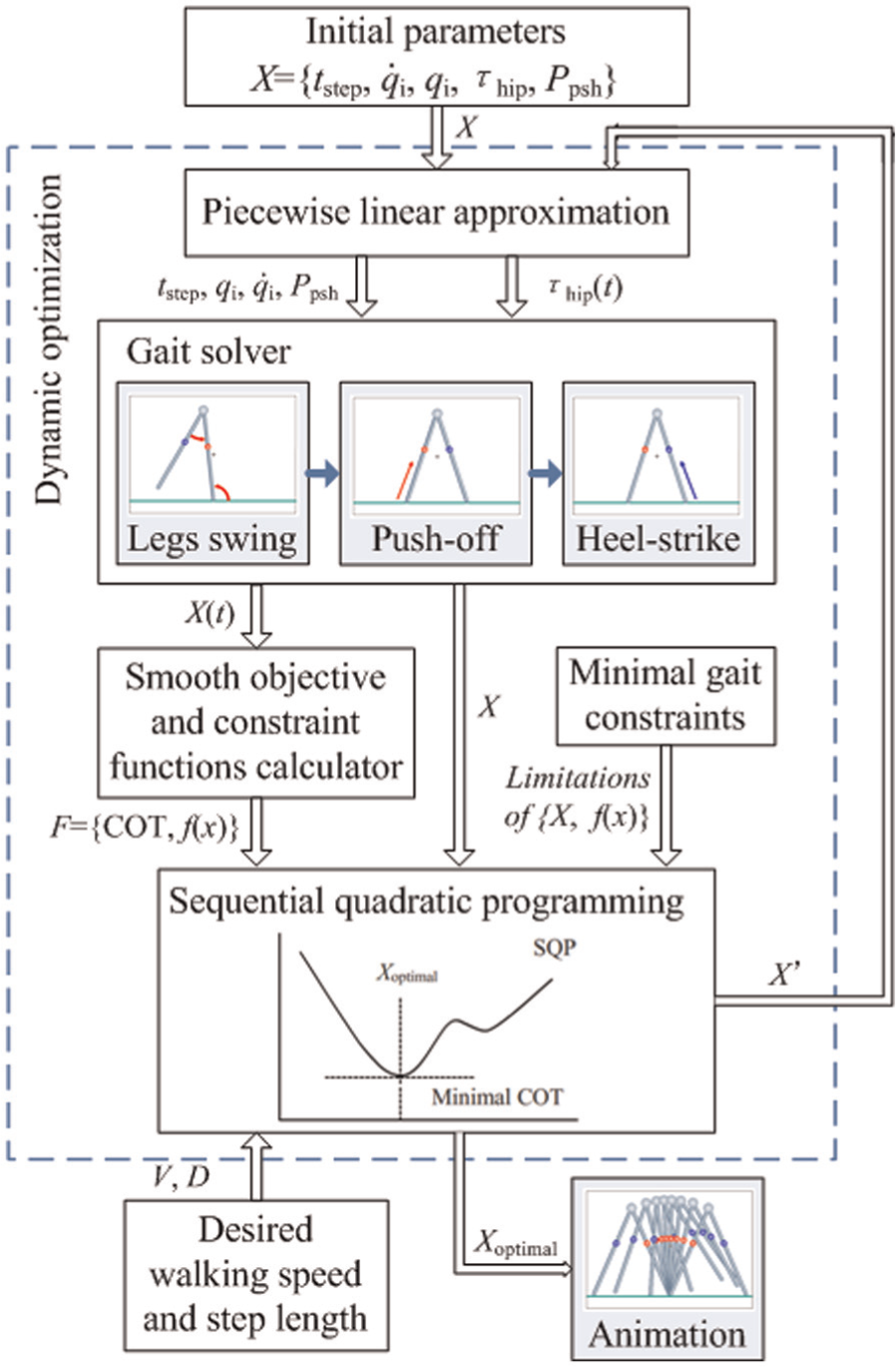
Dynamic optimization control system.

Results and discussions

Analysis of the mechanical parameters

Different mechanical parameters can lead to different walking performances. In this section, we will study the effects of the mass and length distribution on the walking efficiency. The non-dimensional parameters of the mass and length distribution are defined as

$$\{\begin{array}{c}\hfill P_m=\frac{m_l}{m_h}\hfill \\ \multicolumn{1}{c}{P_l=\frac{l_t}{l}}\end{array}$$

(26)

where the mass distribution parameter P_m is the ratio of leg mass m _l and hip mass m_h ; the length distribution parameter P _l is the ratio of the distance between leg centroid and hip l_t and leg length l.

The COT, which is subjected to the constraints D and V, is calculated by varying one of the two distribution parameters while another is fixed. Table 1 shows the range of the parameters in the calculation by considering biological parameters distribution features.^39,40The influence of the variation in the grid points’ number N on the optimal results has been calculated to check the effect of the piecewise linear approximation method. It shows that the minimal COT slightly decreases with the increase in N, but the overall behavior of the optimal results does not change. All the results in this article are non-dimensionalized.

Table 1.

The range of parameters in calculation.

Parameters	Range
Mass distribution parameter Pm	[0.2, 0.5]
Length distribution parameter P l	[0.3, 0.6]
Non-dimensional step length D	[0.3, 1.1]
Non-dimensional walking speed V	[0.3, 0.7]
Number of grid points N	10

For studying the effects of the mass distribution parameter P_m on the COT, we choose two representative fixed values in the range of the length distribution parameter P _l. The values of P _l are 0.3 and 0.5 in Figures 3 and 4, respectively. The two figures show the COT as a function of P_m with various step lengths and two representative fixed walking speeds: (a) V = 0.3 and (b) V = 0.5. The small window in each figure shows the sectional view of the COT versus P_m with fixed step length D. We can see that the COT increases with the increase in P_m when P _l, V, and D are fixed. For a certain set of P _l and V, there will be a corresponding range of D, in which the COT is minimal and P_m has no obvious effect on the COT. For example, with the increase in P_m , the COT is roughly constant as 0.09 when D = 0.4 in Figure 3(a).

Figure 3.

The effects of P_m on COT with fixed P _l = 0.3: (a) V = 0.3 and (b) V = 0.5.

Figure 4.

The effects of P_m on COT with fixed P _l = 0.5: (a) V = 0.3 and (b) V = 0.5.

Figure 4(b) shows that the COT is bigger with short step length than long step length, which is different from Figures 3 and 4(a). This is because the hip joint torque consumes more energy for the leg swinging under the situation of fast walking speed and short step length. (This will be discussed in section “Features of optimal gaits with different walking speed and step length.”) Big value of P _l will lead to high moment of inertia, which is another reason that the hip joint torque consumes more energy.

Figures 5 and 6 show the COT as a function of P _l with the two representative fixed values in the range of P_m , which are 0.3 and 0.5, respectively. We can see that when the step length D is short, the COT increases with the increase in P _l. With the increase in D, the curve of the COT versus P _l gets flat, which indicates that for a certain set of P_m and V, the effect of P _l on the COT is also not obvious within a range of step length D. For long step length, for example, D = 1.0 in Figure 5(b), the COT gradually increases and then decreases with the increase in P _l. The reason of this variation in the COT curve is that with the increase in P _l, the COT _push-off decreases and the COT _swing increases because of the moment of inertia. Meanwhile, the proportion of the COT _swing in the total COT decreases with the increase in the step length. (This will be discussed in section “Features of optimal gaits with different walking speed and step length.”). Therefore, for short step length, the COT increases with the increase in P _l because the COT _swing takes more proportion and it increases with the increase in P _l. However, with long step length, the COT _push-off takes more proportion but it decreases with the increase in P _l, which indicates the nonlinear curve of the COT.

Figure 5.

The effects of P _l on COT with fixed P_m  = 0.3: (a) V = 0.3 and (b) V = 0.5.

Figure 6.

The effects of P _l on COT with fixed P_m  = 0.5: (a) V = 0.3 and (b) V = 0.5.

By comparing Figures 5 and 6 with the same walking speed V, we find that the curves are roughly in similar shape. It indicates that the variation in P_m has no obvious effects on the relation between the COT and P _l.

Features of optimal gaits with different walking speeds and step lengths

The optimal gaits with minimum COT are calculated with the combinations of walking speed V and step length D. Since the qualitative results are not highly sensitive to the model parameter values, ¹⁹ a set of mass and length distribution parameters, P_m  = 0.3, P _l = 0.4, which have relevance to the parameters of biological biped, are chosen for our study.

Figure 7(a) shows that the value of the initial hip angular velocity is bigger than the forward walking speed, and the difference increases with the increase in the step length. This is because with the increase in the step length, the potential energy of the model at the initial position decreases. The hip needs more kinetic energy at the initial position to swing over the midstance.

Figure 7.

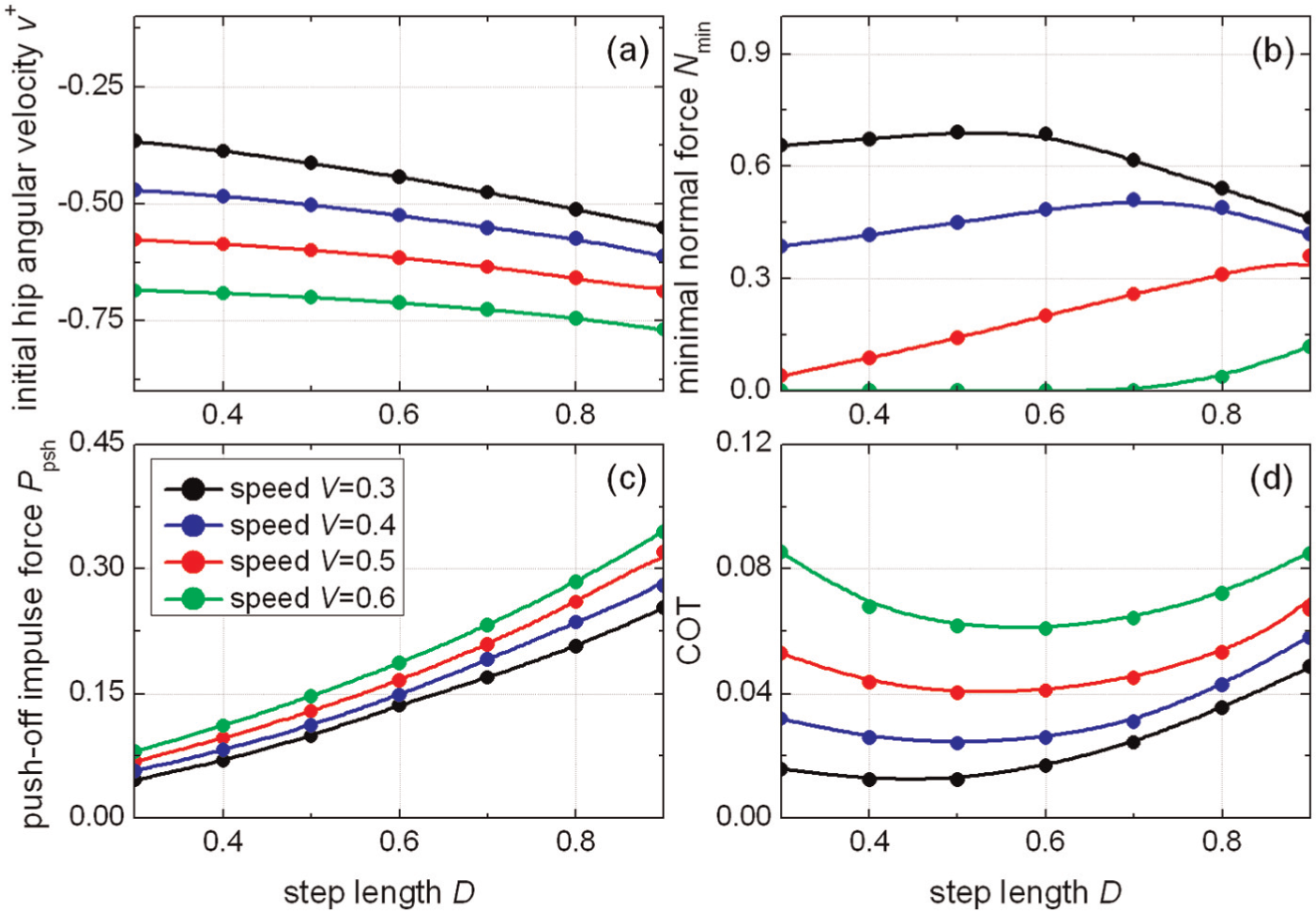
Walking gait features with the combinations of step length and speed: (a) initial hip angular velocity, (b) minimal normal force at stance foot, (c) push-off impulse force, and (d) COT.

The minimal normal force at stance foot N_min during the swing phase (Figure 7(b)) increases with the increase in the walking speed, but increases and then decreases with the increase in the step length. The minimal normal force, which is less than 0, indicates that the stance foot leaves the ground. We find that when the walking speed V is slower than 0.5, the minimal normal force is bigger than 0 with any size of step length (Region I in Figure 8). However, when the walking speed V is faster than 0.5, for example, V = 0.6, short step length (D < 0.7) will lead the minimal normal force to 0. Region II in Figure 8 shows the walking gait of which the minimal normal force is 0. In this case, the hip torque is adjusted to meet the bigger-than-zero requirement, although the COT of the walking increases. Figure 9 shows the normal force at the stance foot during the swing process with fixed walking speed V = 0.6 and different step length, where the horizontal axis is the time divided by the periodic time t_step . The normal force increases and then decreases with the minimal value at the beginning of the step. For the step length D < 0.7, the minimal normal force is 0, while the minimal normal force is bigger than 0 when D > 0.7. We also find that the curves of the normal force with different step length cross at the time points 0.34 and 0.66 and are symmetrical between the two time points.

Figure 8.

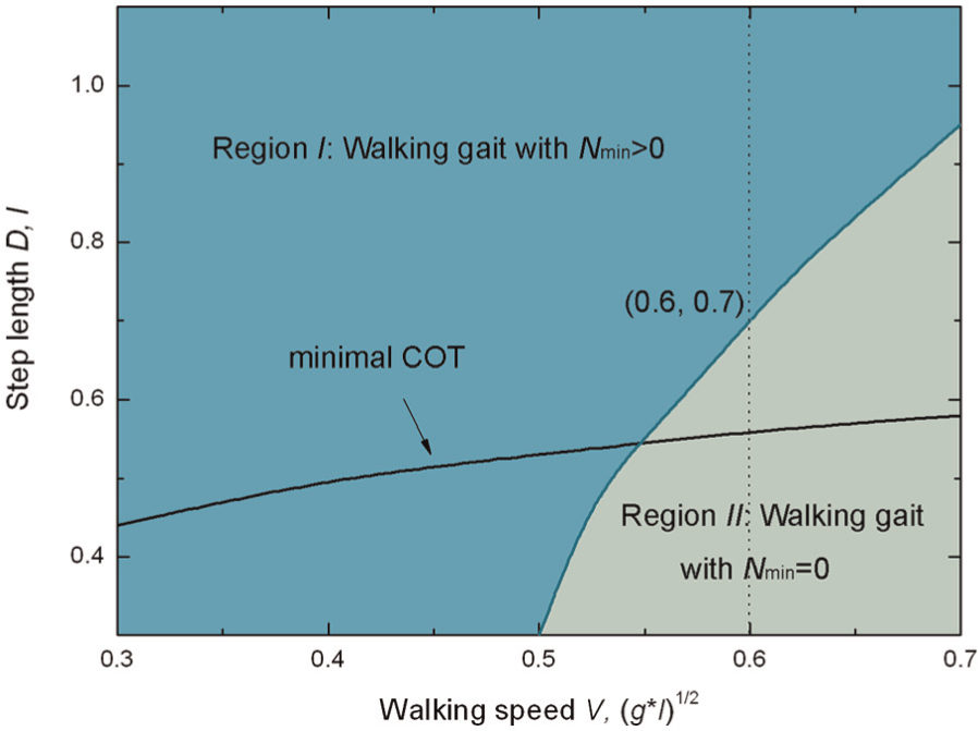
Walking gait region with different N_min and speed–step length relationship for minimal COT.

Figure 9.

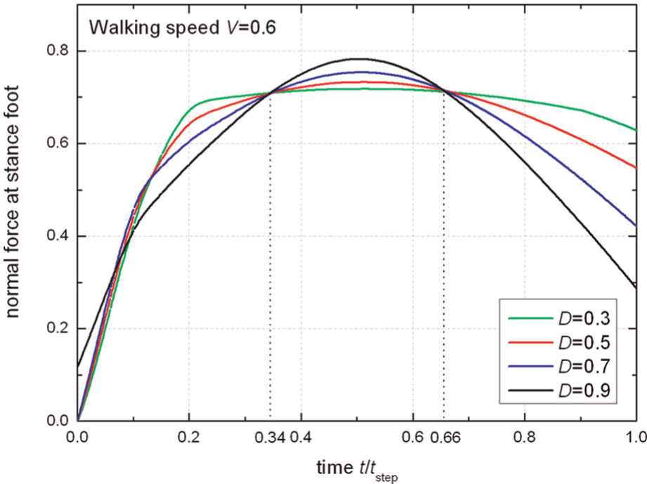
Normal force at stance foot during the swing process (V = 0.6).

The energy cost at push-off COT _push-off is one part of the COT. Figure 7(c) shows that the push-off impulse increases with the increase in the walking speed and the step length. Since the push-off impulse is proportional to the COT _push-off , the COT _push-off will increase with the increase in the walking speed and the step length.

The COT of the optimal gait (Figure 7(d)) increases with the increase in the walking speed. With a certain walking speed, the COT is a quadratic curve with minimal value with the increase in the step length. For example, the minimal COT of the walking with the walking speed V = 0.50 is 0.40 when the step length D = 0.52. This indicates that for a certain walking speed, there will be a walking manner for robots to achieve the most efficient walking. The speed–step length relationship for minimal COT is shown in Figure 8. We can see that the step length for the most efficient walking increases with the increase in the walking speed.

Figure 10 shows the relationship between the total COT and its two parts: COT _push-off and COT _swing . For short step length, the value of the COT _swing is maximal. This is because the angle between the two legs is small, much hip torque energy will be used for accelerating the swing leg to meet the short period time requirement (t _step = D/V). For long step length, strong push-off impulse should be applied for the hip to swing over the midstance. This is the reason that the value of the COT _push-off is maximal with long step length. With the increase in the step length, the COT _push-off increases while the COT _swing decreases (excepting for V = 0.3). This variation relation of the two COT parts explains the quadratic curve of the total COT.

Figure 10.

Total energy cost, energy cost during swing phase and at push-off: (a) V = 0.3, (b) V = 0.4, (c) V = 0.5, and (d) V = 0.6.

For the walking speed V = 0.3 (Figure 10(a)), with the increase in the step length, the COT _swing decreases to 0 at D = 0.6. However, with the continued increase in the step length, the COT _swing increases. This is because that the hip torque output strategy of the optimal gait is changed for long step length and slow walking speed. Figure 11 shows the hip joint torque in the swing process with different step length (V = 0.3). The variation in the area under the hip torque determines the COT _swing . When the step length is shorter than 0.6, the positive hip joint torque at the beginning of the swing phase which is the normal hip torque output strategy can be found. The peak of the hip torque decreases with the increase in the step length (Figure 11(a)–(c)). No hip joint torque is found in the swing phase when D = 0.6. When the step length is longer than 0.6, we find the hip torque at the end of the swing phase. The peak of the hip torque increases and moves to the left with the increase in the step length (Figure 11(d)–(f)).

Figure 11.

Hip joint torque in swing process with different step length (V = 0.3): (a) V = 0.3, D = 0.3; (b) V = 0.3, D = 0.4; (c) V = 0.3, D = 0.5; (d) V = 0.3, D = 0.6; (e) V = 0.3, D = 0.7; and (f) V = 0.3, D = 0.8.

Conclusion

This article investigates the energetic walking gaits with various mechanical parameters and gait feature parameters using a biped walking model with dynamic optimization method.

The effects of the mechanical parameters, including mass and length distribution, on the walking efficiency are studied first. When the length distribution parameter P _l is fixed, the COT of the same walking gait increases with the increase in the length distribution parameter P_m . When P_m is fixed, the COT increases with the increase in P _l for short step length, while for long step length the COT increases and then decreases. For a given value of one of the two distribution parameters, we can find a range of walking speed and step length, in which the variation in another parameter has no obvious effect on the COT.

We also show the features of the optimal walking gaits with the combinations of walking speed and step length. The COT increases with the increase in the walking speed. For a certain walking speed, the COT is a quadratic curve with minimal value with the increase in the step length, which indicates that there is a speed–step length relationship for walking with minimal COT. The total COT is divided into two parts. The energy cost in swing phase mainly decreases and the energy cost at push-off increases with the increase in the step length.

The hip torque output strategy is adjusted in two situations. For fast walking speed and short step length, the hip torque is adjusted to meet the requirement that the minimal normal force at stance foot should be bigger than 0. For slow walking speed and long step length, the hip torque is changed for long distance swing of the swing leg.

These results can help us to understand the mechanism of the energetic walking under various walking situations and design energy-optimal walking bipeds. For example, we can improve the mechanical parameters for energy efficiency when building a biped robot and design efficient leg control and actuator strategies. However, for our purpose of studying the energetic walking bipeds with strong adaptability, we still need to take a lot of further works, such as studying the walking gaits on various slope and the kneed walking.