A novel image zooming method based on sparse representation of Weber’s law descriptor

Abstract

A novel image zooming algorithm based on sparse representation of Weber’s law descriptor is proposed in this article. It is known that features of low resolution can be extracted using four one-dimensional filters convoluting with low resolution patches. Weber’s law descriptor can well deal with local feature, so we extract low-resolution image feature replacing one-dimensional with Weber’s law descriptor in the four filters. In addition, fractional calculus can deal with nonlocal information such as texture. For avoiding small complex component when the size of image is not an odd integer, we modify the extending image method used by Bai, so it can save lots of calculation. The proposed approach combining the Weber’s law descriptor with fractional calculus achieves a very good performance. Experimental results show that our method can well eliminate jagged effect when up-sampling an image and is robustness to noise.

Introduction

The establishment of a modern intelligent transportation system can effectively help to solve the problems of traffic congestion, blocking, and violations, and the license plate recognition system has played an important role in intelligent transportation system. However, when the image acquisition just get a low-resolution (LR) image and it is unsuitable for intelligent recognition, we need to expand the size of the image for further work.

Image zooming aims to restore an image from a degraded image. Applications of super-resolution (SR) image are very important in many fields with the development of modern information technology. The image reconstruction methods can be categorized into four categories: ¹ frequency-domain based methods, ^2,3 example-based methods, ^{4 –7} regularization functional-based methods ^1,8 , and partial differential equation (PDE)-based directional diffusion methods. ^9,10 In this article, we focus on the example-based methods for image reconstruction.

Freeman et al. ¹¹ described a learning-based method that uses generic images in which SR is predicted from LR. The predicting model is learned by adopting a Markov network solved with a belief propagation algorithm. Yang et al. ⁵ proposed an image SR method via sparse representation in which the coefficients between sparse representation for each patch of the LR image are used to get a high-resolution image. The compatibilities among adjacent patches are enforced both globally and locally, while there is a problem that how to determine the optimal dictionary size for natural image patches. Soon, Yang et al. ⁴ introduced a novel coupled dictionary training method based on patch-wise sparse reconstruction, where the learned coupled dictionaries relate to the LR and high-resolution image patch spaces via sparse representation. A fast regression model based on in-place examples was proposed for practical single image SR. ¹² Yin et al. ¹³ proposed a novel method for image SR and fusion, and the method is as follows: For given LR images, up-sampling and decomposing them into low and high frequency components; and then computing and fusing sparse coefficients from the low and high frequency components; reconstructing a high-resolution fused image using the fused sparse coefficients. All aforementioned methods share the same common traits: the LR image is divided into blocks, and the first-order and the second-order gradient is used as the image features. The key problem is how to choose the dictionary and its size. ¹⁴ These methods ignored image nonlocal information, but nonlocal information can help to improve the SR reconstruction performance and fractional calculus can well deal with nonlocal information such as texture. ^1,9,15

Pu ¹⁶ introduced first fractional calculus to image processing and proposed digital images fractional differential mask templates and inhibition principle according to the capabilities of the fractional differential approach for enhancing textural features. Because of the capability of better handling nonlocal features, such as textures, Zhang et al. ^9,15 proposed a fractional diffusion-wave equation for image denoising, and experiments show that the proposed method is effective. Ren et al. ¹ proposed a novel method that combined the local with global features for image zooming, and the experiment results do not suffer from staircase edges block artifacts.

In this article, a novel SR reconstruction method is proposed. The proposed method combines the local operator with the nonlocal operator. The local operator can better handle the textures, and the nonlocal operator has a favorable performance on textures and noise compared to state-of-the-art methods. First, we adopt modified Weber’s law descriptor (WLD) ¹⁷ to describe the image feature instead of the image gradient. The WLD can make use of image local information, which can be used in the sparse representation method for SR. Second, we modify the image denoising method ¹⁸ based on fractional calculus to get a new denoising algorithm. Finally, for further dealing with the texture and reducing the effects of the noise, we enhance image by optimization based on the modified discretization of fractional calculus. Experimental results show that the proposed method has a state-of-the-art performance and do not suffer from staircase effects and noise.

The main contributions of the article are as follows:

A novel image zooming method based on sparse representation is proposed. The method replaces the local filter operator with the WLD, which is modified for considering the weight of each point to the center pixel and eliminating the influence of the noise. The modified WLD can better extract the textures.

Fractional PDE is adopted to smooth the output high-resolution image for removing block effects and noise, and fractional PDE can well deal with the textures and can preserve the image texture structure.

The modified discretization of fractional calculus using Fourier transform can avoid extending four times of the original image and can save lots of computation cost.

The organization of the rest of the article is as follows. In section “Related work,” we give a brief review of the method based on sparse representation. The proposed model and its analysis are introduced in section “Proposed method.” Section “Experiments results” is devoted to implementation details of numerical experiments. Finally, some conclusions are summed up in section “Conclusion.”

Related work

Image super resolution based on sparse representation was first proposed by Yang et al. ⁵ The idea of the method is to obtain the SR image Y from a given image (LR) X using sparse representation. In this method, there are two dictionaries denoted as D_s and D_l, which are trained to have the same sparse representation for each SR and LR image patch pair. For each given LR patch x, a sparse representation will be found with respect to D_l. The corresponding SR patch D_s will be combined according to these coefficients to yield an output SR patch y.

According to hypothesis, the SR image can be represented sparsely in the right over-complete dictionary as

$y=D_s{\alpha }_s\begin{array}{cc}\hspace{0.17em}& \left({\alpha }_s\in R^K,\left|\right|{\alpha }_s\left|\right|<<K\right)\end{array}$

1

where y is a small patch of the SR image Y and α_s is the sparse representation in over-complete dictionary of D_s.

Suppose x is a small patch of LR corresponding to y, and then, x can be sparsely represented as

$x=D_l{\alpha }_l\begin{array}{cc}\hspace{0.17em}& \left({\alpha }_l\in R^K,\left|\right|{\alpha }_l|{|}_0<<K\right)\end{array}$

2

The sparse coefficients α_s can be restricted by representing patches x of the LR image X, with respect to a LR dictionary D_l co-trained with D_s.

For a given image signal x and dictionary D_l, the problem of finding the sparsest representation of x can be formulated as

$\underset{\alpha }{\min }\left|\right|\alpha |{|}_0,\begin{array}{ccc}\hspace{0.17em}& s.t.& \left|\right|{\text{FD}}_l{\alpha }_l-Fx|{|}_2^2\end{array}\le \epsilon$

3

where F is a feature extraction operator or an unit matrix and α is a sparse representation.

Donoho ¹⁹ has shown that as long as the desired coefficients (α) are sufficiently sparse, they can be efficiently reconstructed by minimizing the l₁-norm, as ⁵

$\underset{\alpha }{\min }\left|\right|\alpha |{|}_1,\begin{array}{ccc}\hspace{0.17em}& s.t.& \left|\right|{\text{FD}}_l{\alpha }_{\hspace{0.17em}}-Fx|{|}_2^2\end{array}\le \epsilon$

4

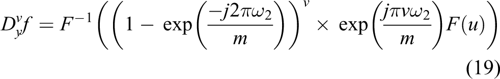
Lagrange multipliers offer an equivalent formulation

$\underset{\alpha }{\min }\left|\right|{\text{FD}}_l{\alpha }_{\hspace{0.17em}}-Fx|{|}_2^2+\lambda |\left|\alpha \right|{|}_1$

5

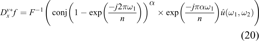
Equation (5) just solves the local image patch optimal solution. However, for each local patch, it does not guarantee the compatibility between adjacent patches. Therefore, for the compatibility, Yang et al. modified equation (4) to be

$\begin{array}{l}\underset{\alpha }{\min }\left|\right|\alpha |{|}_1,\begin{array}{ccc}\hspace{0.17em}& s.t.& \left|\right|{\text{FD}}_l-Fx|{|}_2^2\end{array}\le {\epsilon }_1\\ \begin{array}{cc}\begin{array}{ccc}\begin{array}{cc}\begin{array}{cc}\hspace{0.17em}& \hspace{0.17em}\end{array}& \hspace{0.17em}\end{array}& \hspace{0.17em}& \hspace{0.17em}\end{array}& \hspace{0.17em}\end{array}\left|\right|\widehat{\text{F}}\text{D}s{\alpha }_{\hspace{0.17em}}-\omega |{|}_2^2\le {\epsilon }_2\end{array}$

6

where matrix $\widehat{F}$ extracts the region of overlap between previously reconstructed SR image and the current objective patch, and ω contains the values of the previously restored SR image on the overlap. Equation (6) can be simplified as

$\underset{\alpha }{\min }{\left|\right|\tilde{D}\alpha -\tilde{x}\left|\right|}_2^2+\lambda \left|\right|\alpha |{|}_1$

7

where $\tilde{D}=\left[\begin{array}{l}F{D}_l\\ \beta \widehat{F}{D}_s\end{array}\right]$ , $\tilde{x}=\left[\begin{array}{l}Fx\\ \beta \omega \end{array}\right]$ , and β controls the trade-off between finding a SR patch and matching the given LR image. Generally, we select β = 1. Since obtaining an optimal solution α* of equation (6), the SR patch can be reconstructed as y = D_sα*.

But equations (4) and (6) do not demand exact equality between the LR patch x and its restoration D_lα. For eliminating this discrepancy by projecting Y₀ onto the solution space of SHY = X, we can obtain more accurate SR image by computing equation (8) using the back-projection method

$Y^{*}=\underset{Y}{\arg \min }\left|\right|\text{SHY}-X|{|}_2^2+\gamma ||Y-Y_0|{|}_2^2$

8

where S represents for a blurring filter and H stands for down-sampling operator.

Proposed method

Weber’s law descriptor

In this section, we will briefly review the feature extracting method proposed in the study by Yang et al. ⁵ and discuss the model of the WLD. For illustrating that WLD can well be used to extract feature, we carry out an experiment of WLD compared with the method by Yang. ⁵

From the view of perception, humans are more sensitive to the details of the high frequency details than that of the low frequency of an image. Generally, Gauss filter is used as a feature extraction operator in equation (3). Experimental results show that it is feasible to reconstruct a high-resolution image using the high frequency part of a LR image. Many researchers suggest that different features of LR images should be extracted to ensure the precision of prediction. Freeman et al. ¹¹ extracted edge information of LR as the features using a high-pass filter. Sun et al. ²⁰ extracted the contour of LR as the features using a set of Gauss iterative filters.

In the method by Yang, ⁵ there are four one-dimensional filters for extracting the features as follows ²¹

$\{\begin{array}{l}{f}_1=[-1,0,1],\begin{array}{cc}\begin{array}{cc}\hspace{0.17em}& \hspace{0.17em}\end{array}& f_2=f_1^T\end{array}\\ f_3=[1,0,-2,0,1],\begin{array}{cc}\hspace{0.17em}& f_4=f_3^T\end{array}\end{array}$

9

Four groups feature vectors convoluting four filters with the LR blocks were first obtained, and then, grouped the four sets of vectors together to get the final feature of the LR image blocks. There, we get a good compatibility between reconstructed high-resolution image blocks and the surrounding blocks.

WLD was proposed for extracting local area features by Chen et al. ¹⁷ and motivated by Weber’s law. Weber, a German physiologist, ^22,23 first described Weber’s law in 19th century. The law reveals that the ratio of the background stimulus u to the intensity increment δu is a constant. ²⁴ This relationship can be expressed as

$\frac{\delta u}{u}=\text{const}$

10

WLD is based on a physiological law, it has three advantages: detecting edges elegantly, robustness to illumination change and noise, and its powerful representation ability. ¹⁷ It consists of differential excitation and orientation. Differential excitation (ω) is a function of the Weber fraction and orientation (θ) is a gradient orientation of the current pixel.

The changes of the current pixel can be described by intensity differences between its neighbors and a current pixel. So the step of computing a differential excitation ω(I_c) of the current pixel comes to be as follows: computing the differences between the center point and its neighbors is the first step

$\Delta I_i=I_i-I_c$

11

where I_i stands for the intensities of p neighbors of I_c, i = 0,1,…, p−1. p is the number of p neighbors.

The second step is computing the arctangent of the sum of differences ΔI_i

$\omega \left(I_c\right)=\arctan \left[{\displaystyle \sum _{i=0}^{p-1}\frac{\Delta I_i}{I_c}}\right]$

12

where p stands for the number of p neighbor and ΔI_i have different values when p has different values.

For considering the weight of each point to the center pixel, in this article, we modified the formulation of ΔI_i. We adopt p₁ = 12 and p₂ = 8 in this article, then we get $\Delta I_m^{p_1}$ and $\Delta I_n^{p_2}$ , finally, ΔI_i is computed using following equation

$\Delta I_i=w_1\times \Delta I_m^{p_1}+w_2\times \Delta I_n^{p_2}$

13

where w₁ and w₂ represent different weights on the neighborhood p₁ and p₂, respectively.

We will carry out an experiment for extracting the textures of an image using WLD. For a given image, we first compute the image differential excitation and then make sure the gradient direction according to gradient difference. Finally, we show the differential excitation by mapping it to [0,255]. Figure 1 shows the comparison result of different filters, and we can see that the result of the WLD is better than that of other filters in extracting textures.

Figure 1.

Comparison of the different filters. (a) “Barbara” original image. (b) Filtered image using WLD. (c) Filtered image using the first filter f₁. (d) Filtered image using the second filter f₂. (e) Filtered image using the third filter f₃. (f) Filtered image using the fourth filter f₄. (g) Filtered image using the grouped four filters. WLD: Weber’s law descriptor.

Modified method of fractional calculus

In this section, first, we give a discussion of calculus from integer to fractional calculus. Then, discrete fractional calculus adopting frequency domain definition is introduced. Finally, we improve the discretization method introduced in the study by Bai and Feng. ¹⁸ We will carry out experiments to show that the modified method is effective and has a less computation cost than that of the method by Bai and Feng. ¹⁸

As we all know, fractional calculus is an extent of integer calculus, and the definition of fractional calculus has many formulations, such as definition Rieman–Liouville, Caputo, Weyl, and Grünwald–Letnikov. ^1,9,18,25 In this article, we adopt frequency domain definition for considering fractional calculus is easy to compute.

For a given function $f\left(t\right)\in L^2\left(R\right)$ , the Fourier transform of f(t) is defined as

$\widehat{f}\left(w\right)={\displaystyle {\int }_{\hspace{0.17em}}f\left(t\right)e^{-jwt}}\text{d}t$

14

The equivalent formulation of the first-order derivative in the frequency domain is

$Df\left(t\right)\leftrightarrow \left(jw\right)\widehat{f}\left(w\right)$

15

From equations (16) and (17), we can extend the integer-order Fourier transform to a fractional one. For a fraction number v, we can obtain the fractional derivative of f(t) in the frequency domain with

$D^{v}f\left(t\right)\leftrightarrow {\left(jw\right)}^v\widehat{f}\left(w\right)$

16

Similarly, we can get forms of the fractional-order partial derivative of $f\left(x,y\right)\in L^2\left(R^2\right)$ as follows ^1,18

$\begin{array}{l}{D}_x^{v}f\left(x,y\right)\leftrightarrow {\left(j{w}_1\right)}^v\widehat{f}\left(w_1,w_2\right)\\ D_y^{v}f\left(x,y\right)\leftrightarrow {\left(j{w}_2\right)}^v\widehat{f}\left(w_1,w_2\right)\end{array}$

17

Now, we can define the fractional gradient operator ${\nabla }^{v}f=\left(D_x^{v}f,D_y^{v}f\right)$ and get the corresponding magnitude $\left|{\nabla }^{v}f\right|=\sqrt{{\left(D_x^{v}f\right)}^2+{\left(D_y^{v}f\right)}^2}$ .

There are many methods to implement the fractional order differential. Here, we adopt frequency domain definition introduced by Bai and Feng. ¹⁸ $D_x^v$ and $D_y^v$ are the fractional order derivatives of order v for the given images f(size of m × m). ¹ Two-dimensional discrete center difference Fourier transforms are defined as

$D_x^{v}f=F^{-1}\left({\left(1-\text{exp}\left(\frac{-j2\pi {\omega }_1}{m}\right)\right)}^v\times \text{exp}\left(\frac{j\pi v{\omega }_1}{m}\right)F\left(u\right)\right)$

18

$D_y^{v}f=F^{-1}\left({\left(1-\text{exp}\left(\frac{-j2\pi {\omega }_2}{m}\right)\right)}^v\times \text{exp}\left(\frac{j\pi v{\omega }_2}{m}\right)F\left(u\right)\right)$

19

and the adjoints of $D_x^{v}u$ and $D_y^{v}u$ , respectively, are

$D_x^v{\hspace{0.17em}}^{\ast }f=F^{-1}\left(\text{conj}{\left(1-\exp \left(\frac{-j2\pi {\omega }_1}{n}\right)\right)}^{\alpha }\times \exp \left(\frac{-j\pi \alpha {\omega }_1}{n}\right)\widehat{u}\left({\omega }_1,{\omega }_2\right)\right)$

20

$D_y^v{\hspace{0.17em}}^{\ast }f=F^{-1}\left(\text{conj}{\left(1-\exp \left(\frac{-j2\pi {\omega }_2}{n}\right)\right)}^{\alpha }\times \exp \left(\frac{-j\pi \alpha {\omega }_2}{n}\right)\widehat{u}\left({\omega }_1,{\omega }_2\right)\right)$

21

When m is an odd integer, $D_x^{v}f$ is a real value; when m is an even integer, $D_x^{v}f$ is not a real value. ¹⁸ In order to avoid the emergence of complex components, Bai extended the size of the original image. The size of the extended image is $\left(2m+1\right)\times \left(2m+1\right)$ , that is, four times size of the original image. This extending method will increase the amount of calculation. So, we need to modify the extended methods for less computation. When m is an even integer, we extend the size of the image size to be $\left(m+1\right)\times \left(m+1\right)$ . When converting the image from the frequency domain to the spatial domain, we will subtract the row and the column of which we extended at the right column and bottom row. In order to verify the validity of the extending method, we design an experiment as follows. First, we add one row at the bottom of the original image γ and add one column at the right of the previous step image and transform the original image to image γ′. Second, with Fourier transform, we transform image γ′ to β, with β, do inverse Fourier transform. Finally, we check the pixel gray value of the same position and same size in the original image to see whether the result image is modified or not. To validate feasibility of our method, we carry out two experiments on the image as shown in Figure 2(a). We can see that the images have the same pixel values after performing modified fractional calculus method from Figure 2. The signal noise ratio (SNR) results of our method and the method by Bai and Feng ¹⁸ are listed as in Table 1. Figure 2 shows that the data are the same before and after transformation. Table 1 shows that the computation time and SNR results of our method are superior to that of the method by Bai and Feng. ¹⁸ We can see that the computation cost of our modified method is much less than that of the method by Bai and Feng ¹⁸ with the increasing iteration, while SNR value of our modified method is a little bigger than the result of Bai and Feng. ¹⁸ The code of the study by Bai and Feng were obtained from the author Bai. The two experiments are carried out on the same environments in which the operating system is Microsoft Windows 7 ultimate edition (Service Pack 1), CPU is Intel® Core™ i3-2120 @3.30 GHz, 8.00 GB of memory.

Figure 2.

(a) “Lena” original image, (b) pixel gray values of the selected rectangular in the original image (a), (c) the lower left is result image (output) that performs Fourier transform and inverse Fourier transform, (d) pixel gray values of the selected rectangular in the result image after performing modified fractional calculus (c).

Table 1.

Computation time and SNR results of our method and the method by Bai and Feng. ¹⁸

	Method by Bai and Feng 18		Modified
Iterations	Time (s)	SNR (dB)	Time (s)	SNR (dB)
50	27.66	28.4653	5.6	28.6784
100	54.48	24.6525	10.64	25.4809
200	107.33	21.3652	21.52	22.9701
500	268.64	18.1451	52.06	19.9944
1000	583.81	15.9336	103.63	17.7287
2000	1261.44	13.5464	207.56	15.2781

SNR: signal noise ratio.

We can see that the cost of computation of the method by Bai and Feng ¹⁸ and modified method is increasing and SNR values are decreasing when the numbers of the iteration increasing from Table 1. While the time of the method by Bai and Feng ¹⁸ is almost five times of the modified method, and the SNR values of the method by Bai and Feng ¹⁸ are smaller than modified method. This shows that the modified method not only save the computation time and also can get larger SNR values.

The scheme of the proposed method

The process of the proposed algorithm can be described as follows:

Initialization: input the LR image X, dictionary D_l of LR, dictionary D_s of high resolution, and other related parameters;

Iteration for each patches of X.

Feature extracting: Extract the WLD feature ω(I_c) of LR image using equation (12).

To recover each LR patch and get sparse representation α according to x = D_lα, where α must be satisfied the optimization problem: $\underset{\alpha }{\min }\left|\right|\omega \left(I_c\right)D_l{\alpha }_{\hspace{0.17em}}-\omega \left(I_c\right)x|{|}_2^2+\lambda |\left|\alpha \right|{|}_1$ .

To compute the high-resolution image patches using y = D_sα, put the high-resolution image patches into a high-resolution image Y₀.

End for iteration.

Image reconstruction: Use the back-projection method to find the closest image to expected image that satisfies the reconstruction constraint as equation (8)

$Y^{*}=\underset{Y}{\arg \min }\left|\right|\text{SHY}-X|{|}_2^2+\gamma ||Y-Y_0|{|}_2^2$

• 5. Output the high-resolution image Y′ using the following equation

$\frac{\partial Y^{\prime }}{\partial t}=\text{div}\left(c\left(|{\nabla }^v{Y}^{\prime }{|}^2\right){\nabla }^v{Y}^{\prime }\right)+\lambda Y^{*}$

22

where Y′ is the final result.

In the proposed method, the first step is we input the LR image, dictionary size, image patch size, numbers of patches to sample, dictionaries of LR, and high resolution, which can be pretrained using many different types of images. The second step begins an iteration, for each patches of the LR image X, we first extract features of the LR image patches using differential excitation equation (12) of the modified WLD introduced in section “Weber’s law descriptor.” The parameter p in equation (12) is selected to be 8 and 12, respectively. Second, each LR patch is recovered according to the features obtained in the second step, and the high-resolution image patches are generated by solving the optimization problem: $\underset{\alpha }{\min }{\left|\right|\tilde{D}\alpha -\tilde{y}\left|\right|}_2^2+\lambda \left|\right|\alpha |{|}_1$ , then put the high-resolution patch y into a high-resolution image Y₀. End iteration until all patches of X was computed. The fourth step can described as: the back-projection method is employed to find the closest image to the expected image, which satisfies the reconstruction constraint equation (8). In the fifth step, for better dealing with nonlocal feature, we process the closest image got in the fourth step using equation (22), in which we modified fractional calculus discretization method that is explained in section “Modified method of fractional calculus,” and it cannot only deal well with textures but also save computation cost. The output image we obtained contains more texture but less blurring and zigzag because our method not only considers the local features but also takes into account the nonlocal features.

Experimental results

In this section, we will compare the output images of our proposed method with that of one of the up-sampling algorithms (bilinear interpolation (BLI), ²⁶ the bicubic interpolation (BCI), ²⁷ the traditional super-resolution method of sparse representation (SCSR) ⁵ ), the decorrelated vectorial total variation (DVTV ²⁸ ), the structure tensor total variation ²⁹ , and the Hessian Schatten-norm Poisson Image Reconstruction by Augmented Lagrangian (HSPIRAL ³⁰ ). The experimental environment is set as: operating system is Microsoft Windows 7 ultimate edition (Service Pack 1), CPU is Intel® Core™ i3-2120 @3.30G Hz, 8.00 GB of memory. First, we enlarge the parts of the input LR image by a factor of 4; then test effects of the magnification factor; third, verify the robustness to noise; and finally, analyzing effects of the dictionary size. All the test images are downloaded from the Web site: https://www.cs.cmu.edu/∼cil/v-images.html. The images tested in the experiments are Barbara, Lena, butterfly, leaves, parrot, liberty statue, and plants.

The formula of peak SNR (PSNR) and root mean square error (RMSE), respectively, is

$\text{PSNR}=10\times \text{log}\left(\frac{{255}^2}{\text{MSE}}\right),\text{ MSE}=\frac{1}{mn}{\displaystyle \sum _{i=1}^m{\displaystyle \sum _{j=1}^n{\left|\right|I\left(i,j\right)-K\left(i,j\right)\left|\right|}^2}},\text{ RMSE}=\sqrt{\text{MSE}}$

where I and K represent input and output images, respectively.

Selection of fraction number v

In this subsection, we will discuss the selection of the fraction number v. Different values of v can introduce different results. In this experiment, the discussed range of v is [0.2, 1.9] for different images, and the performance evaluation employs the PSNR and RMSE. The bigger the PSNR’s value, the better the result of the restored image is. On the contrary, the smaller the RMSE’s value, the better the result of the restored image is. We have tested seven images for selecting proper fractional order v and computed the values of PSNR and RMSE when v has different values. We can see that PSNR achieves the largest and RMSE gets the smallest when value of v floating around 0.8 as seen from Table 2. Therefore, we will adopt the value of v as 0.8 in this article.

Table 2.

Value of PSNR and RMSE when adopting different value of v.

Image	Butterfly		Hat		Peppers		Lena		Leaves		Plants		Parrot
v	PSNR	RMSE	PSNR	RMSE	PSNR	RMSE	PSNR	RMSE	PSNR	RMSE	PSNR	RMSE	PSNR	RMSE
0.2	57.6392	0.4722	59.8710	0.3552	53.6959	0.7478	61.8645	0.2910	60.6077	0.3295	64.5989	0.2115	61.8991	0.2869
0.3	57.6351	0.4716	59.8828	0.3558	53.6886	0.7482	61.8991	0.2898	60.6019	0.3294	64.6729	0.2105	61.8411	0.2883
0.4	57.6168	0.4733	59.8779	0.3558	53.6920	0.7479	61.9007	0.2893	60.6312	0.3288	64.6610	0.2101	61.8614	0.2881
0.5	57.6469	0.4725	59.8571	0.3563	53.6906	0.7479	61.9276	0.2892	60.5867	0.3289	64.6521	0.2106	61.8818	0.2871
0.6	57.6245	0.4732	59.8878	0.3559	53.6982	0.7474	61.9039	0.2902	60.5867	0.3285	64.664	0.2108	61.8489	0.2875
0.7	57.6239	0.4723	59.8958	0.3555	53.6998	0.7474	61.8944	0.2905	60.5995	0.3292	64.6313	0.2109	61.8505	0.2876
0.8	57.6671	0.4711	59.9247	0.3545	53.6975	0.7475	61.9372	0.2888	60.6584	0.3273	64.7636	0.2083	61.8975	0.2866
0.9	57.6594	0.4716	59.8868	0.3562	53.6941	0.7476	61.9039	0.2898	60.5913	0.3305	64.6283	0.2104	61.8834	0.2874
1	57.6499	0.4722	59.5948	0.3558	53.6972	0.7474	61.9070	0.2897	60.6159	0.3299	64.6283	0.2102	61.8928	0.2870
1.1	57.6612	0.4713	59.8858	0.3562	53.6943	0.7476	61.9102	0.2896	60.5820	0.3305	64.6402	0.2099	61.8724	0.2876
1.2	57.6286	0.4714	59.8828	0.3561	53.6978	0.7475	61.9292	0.2893	60.5890	0.3288	64.6402	0.2105	61.9023	0.2864
1.3	57.6203	0.4727	59.8640	0.3556	53.6972	0.7476	61.8771	0.2907	60.5890	0.3294	64.6224	0.2108	61.8692	0.2875
1.4	57.6004	0.4731	59.8838	0.3555	53.6969	0.7474	61.8818	0.2900	60.6195	0.3283	64.6670	0.2105	61.8505	0.2878
1.5	57.6410	0.4729	59.8789	0.3562	53.6963	0.7476	61.9244	0.2895	60.6183	0.3288	64.6879	0.2099	61.8975	0.2871
1.6	57.6414	0.4728	59.8719	0.3559	53.6939	0.7478	61.9039	0.2895	60.6418	0.3284	64.7090	0.2093	61.8865	0.2869
1.7	57.6203	0.4727	59.8819	0.3562	53.6951	0.7475	61.8897	0.2900	60.5762	0.3303	64.6372	0.2105	61.8598	0.2872
1.8	57.6481	0.4719	59.8532	0.3565	53.6879	0.7480	61.8849	0.2905	60.589	0.3290	64.6640	0.2102	61.863	0.2876
1.9	57.6174	0.4728	59.8473	0.3568	53.6918	0.7480	61.8897	0.2901	60.6065	0.3290	64.6849	0.2101	61.8912	0.2870

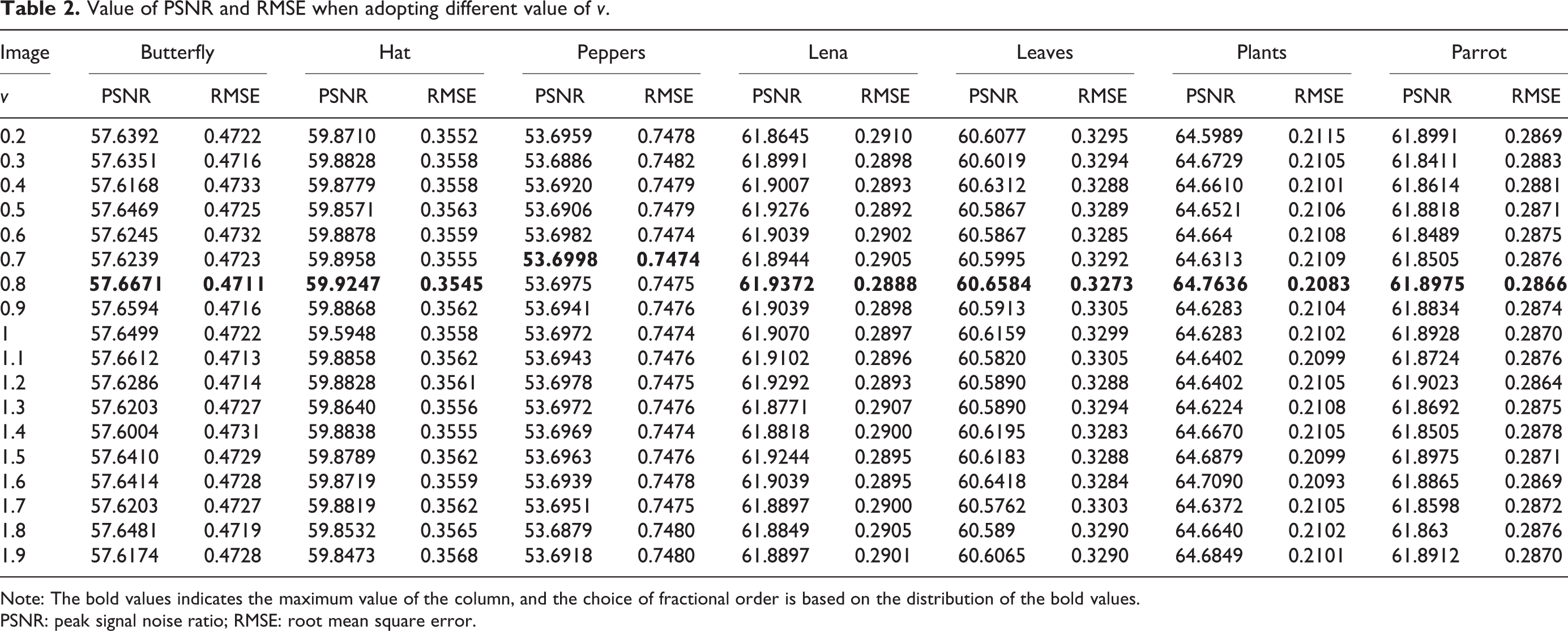
Note: The bold values indicates the maximum value of the column, and the choice of fractional order is based on the distribution of the bold values.

PSNR: peak signal noise ratio; RMSE: root mean square error.

Image super resolution

The outputs of our method along with methods of BLI, ²⁶ BCI, ²⁷ DVTV, ²⁸ Weber²², and SCSR ⁵ are shown in Figure 3. The key idea of the BLI is first to perform the linear interpolation in one direction and then in the other direction. Though each step is linear in the sampled values and in the position, the interpolation as a whole is not linear but rather quadratic in the sample location. In contrast to BLI, which only takes 4 pixels into account, BCI considers 16 pixels. Therefore, images up-sampled with BCI have fewer interpolation artifacts and are smoother. We can see there are many jagged effects in the first column and not clear enough except for the image (p). There are less jagged effects in the outputs of SPSR than the result of BCI but have undesired smoothing (we choose patch size as 5 × 5 pixels and dictionary size 512), especially in “butterfly” image. Because the method of Weber²² aims at gray image, so there are some shortcomings when it is used for processing color images. We will see double edges in result images of method by Weber. ²² In Figure 3(q), the original color of the area of we select is close to gray and white, but the color after zooming is distortion, so the results of the method by Wang et al. ⁸ is the worst in this experiment. The results have the almost same clear texture in the images (h) and (k), and the output image (n) is the worst. We computed the PSNR and RMSE of the method mentioned earlier, and we can see that the PSNR value is the biggest and the RMSE value is the smallest in the results of this method. So, we can state that the output images of our proposed method have lesser jagged effects and well dealt with background image (p = 8 in equation (13)). We plot a curve for three images’ PSNR using six methods, it shows that PSNR of our method is the biggest from Figure 4.

Figure 3.

Results of the images magnified with a factor of 4. (a–c): BLI, PSNR = 36.5053, 40.3627, 41.4907, RMSE = 8.091, 4.8022, 3.4463; (d–f): BCI, PSNR = 33.1309, 37.1606, 37.6421, RMSE = 13.0153, 7.9019, 6.0192; (g–i): SCSR, PSNR = 40.2745, 53.2414, 45.5901, RMSE = 3.5732, 2.5484, 1.9224; (j–l): our method, PSNR = 40.3212, 44.1811, 46.5835, RMSE = 3.5659, 2.2878, 1.7318; (m–o): method by Ono and Yamada, PSNR = 32.9813, 35.2006, 35.4041, RMSE = 4.2273, 3.5658, 3.4674 ²⁸ ; and (p–r): method by Wang et al., ⁸ PSNR = 22.2222, 27.9341, 26.2997, RMSE = 19.7437, 10.2290, 12.3468.

Figure 4.

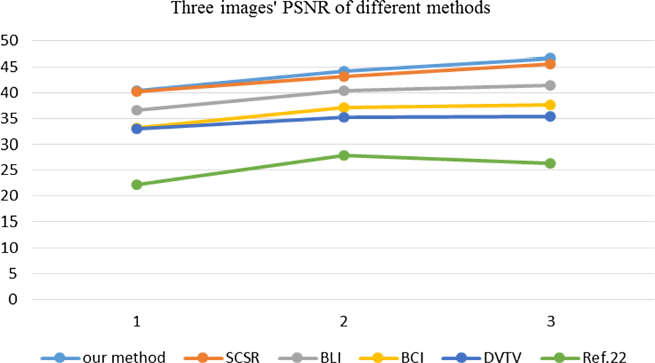
PSNR of three images of six methods. PSNR: peak signal noise ratio.

Effects of magnification factor

For validating the effectiveness of our proposed method, we up-sample portion of the “parrots” image with different magnification factors, such as 2, 3, 4, and 5. The results of the BCI method, SCSR ⁵ method, DVTV ²⁸ method, and the proposed method are shown in Figure 5. When taking the magnification factor as 2, almost there exist not any differences between the results of these three methods. When taking the magnification factor as 3, there are some differences between the results of these three methods. The result of the BCI method is less clear than that of SCSR and the proposed methods. The color of the area of we select is distorted in the result of the study by Wang et al., ⁸ because the method by Wang et al. ⁸ aims at image zooming of the gray image. As the magnification factor value increases, the results of SCSR and the proposed methods are clear than that of bicubic’s. The texture of the proposed method is clear than that of SCSR method. There are some zigzags in the result of the algorithm DVTV, ²⁸ and as the magnification factor raises, the jagged phenomena are increasingly evident. But the texture of the method described in this article does not.

Figure 5.

Performances evaluation of our proposed method with different magnification factors. (a–d): BLI, ²⁶ PSNR = 40.8793, 40.4315, 40.3627, 40.3066, RMSE = 4.1283, 4.6531, 4.8022, 4.8733; (e–h): SCSR, ⁵ PSNR = 41.9838, 42.8629, 43.2414, 43.5568, RMSE = 3.04 93, 2.6704, 2.5484, 2.4557; (i–l): DVTV, ²⁸ PSNR = 31.3349, 33.7491, 35.2006, 36.4023, RMSE = 4.1363, 3.7435, 3.5658, 3.4195; (m–p): proposed method, PSNR = 42.0961, 43.0331, 44.1811, 43.6948, RMSE = 2.9779, 2.6038, 2.2878, 2.4128; (q–t): method by Wang et al., ⁸ PSNR = 25.2455, 26.9764, 27.9341, 28.9267, RMSE = 13.4668, 11.4214, 10.229, 9.1244, respectively, and from left to right are with magnification factors of 2, 3, 4, and 5. PSNR: peak signal noise ratio.

Effects of noise

To verify the robustness of our proposed method against noise, we test the LR image with different levels of standard deviation of Gaussian noise from 5 to 20. Figure 6 shows the outputs of our proposed method applying to the Liberty statue images with different levels of Gaussian noise. As the noise level increases, different effects exhibit in the results of different methods. There are small differences and removed influence of noise in the first column except of SCSR. When the level of Gaussian noise increases to 10, BLI and BCI methods have almost the same results and are poor of robustness, and the output image with SCSR method has many noises in it and is the worst case among the results with these four methods in the second column. When the noise level being set to be 15 or 20, the results of BLI, BCI, DVTV, and SCSR have many noises among the output images. In these levels of noise, there are some noises in the output image of our proposed algorithm too, but it is the best result of these methods. Table 3 also shows that proposed algorithm achieves the lowest RMSE among these methods as well.

Figure 6.

Performances evaluation of our method on noisy data. Noise level (standard deviation of Gaussian noise) from left to right: 5, 10, 15, and 20. (a–d): results of BLI; (e–h): results of BCI; (i–l): outputs of SCSR; (m–p): denoised images using our method; and (q–t): method by Chan et al. ³

Table 3.

The RMSEs of reconstructed images from different levels of noisy inputs.

Noise levels/Gaussian σ	0	5	10	15	20
Our method	1.4546	2.3636	3.8168	5.0708	6.4555
Bicubic	1.9358	2.6015	3.8976	5.3842	6.8784
Bilinear	1.9624	2.6945	3.9047	5.4053	6.9383
Yang 5	2.2624	2.8945	4.1794	5.5564	6.9970
DVTV 28	3.4434	4.4367	4.8396	5.6187	7.3477

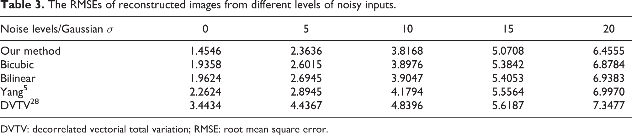
DVTV: decorrelated vectorial total variation; RMSE: root mean square error.

Effects of dictionary size

Less dictionaries should possess less expressive power and may get a less accurate approximation but less computing cost. In this section, we will evaluate the effect of the dictionary size on image SR. We train eight dictionaries with size of 16, 32, 64, 128, 256, 512, 1024, and 2048 from the sampled 10,000 images. Table 4 shows the reconstructed results for five images (including leaves, liberty statue, parrots, plants, and butterfly image) using dictionaries with different sizes. The lower the RMSEs are, the better the reconstructed images. The results of our algorithm for these five images are lower than that of SCSR except few numerical values. The results of SCSR method are relative stability as the dictionary size increasing, while the result of our algorithm doesn’t. Fluctuation of the results of SCSR is bigger when the dictionary size increasing from 512 to 1024 and 2048. According to the study by Yang et al., ⁵ we knew that the bigger the size of the dictionary, the more accurate approximation is, but the more computation cost. Larger dictionary sizes should increase the computation cost, but the RMSE have changed little in proposed method in this article. So, we always fix the dictionary size as 64 in all our experiments for a balance between image quality and computation cost.

Table 4.

Results of our algorithm compared to SCSR ⁵ and the corresponding RMSEs.

images\mse\dictionary size	Leaves		Liberty statue		Parrots		Plants		Butterfly
	Proposed	SCSR 5	Proposed	SCSR 5	Proposed	SCSR 5	Proposed	SCSR 5	Proposed	SCSR 5
16	3.5623	4.2736	1.4546	3.0528	2.6083	2.9756	1.9416	2.7256	4.1346	4.4470
32	3.5161	4.3064	1.433	3.0359	2.5635	2.9799	1.9301	2.7247	4.0837	4.4802
64	3.4582	4.2589	1.4228	3.0534	2.5470	2.9848	1.9028	2.7213	4.0231	4.4544
128	3.5064	4.2297	1.4204	3.0386	2.5357	2.9566	1.9038	2.7038	4.0448	4.3953
256	3.5088	4.1827	1.4213	3.0416	2.5394	2.9479	1.9249	2.7040	4.0312	4.3864
512	4.3187	4.1959	1.5598	3.0358	2.8725	2.9488	2.1994	2.7029	4.2844	4.3747
1024	4.015	4.1711	1.4927	3.0280	2.5188	2.9505	2.1951	2.6997	4.1806	4.4145
2048	4.0225	4.1845	1.5342	3.0317	2.7187	2.9494	2.1019	2.7045	4.1430	4.3853

SCSR: super-resolution method of sparse representation; RMSE: root mean square error

Conclusion

In this article, a novel algorithm is proposed toward the single image super-resolution based on WLD and fractional calculus. The idea is based on that nonlocal information such as texture can be well dealt with fractional calculus, the modified discretization of fractional calculus not only can save lots of computation cost but also can well deal with nonlocal information; and the local information can be extracted using Weber’s law descriptor, the modified WLD can well extract textures and avoid effects of noise. Experimental results show that our presented method is effective for eliminating jagged effect and removing noise. In the future work, we will try to fuse the extraction method with other algorithms.