Deterministic learning enhanced neutral network control of unmanned helicopter

Abstract

In this article, a neural network–based tracking controller is developed for an unmanned helicopter system with guaranteed global stability in the presence of uncertain system dynamics. Due to the coupling and modeling uncertainties of the helicopter systems, neutral networks approximation techniques are employed to compensate the unknown dynamics of each subsystem. In order to extend the semiglobal stability achieved by conventional neural control to global stability, a switching mechanism is also integrated into the control design, such that the resulted neural controller is always valid without any concern on either initial conditions or range of state variables. In addition, deterministic learning is applied to the neutral network learning control, such that the adaptive neutral networks are able to store the learned knowledge that could be reused to construct neutral network controller with improved control performance. Simulation studies are carried out on a helicopter model to illustrate the effectiveness of the proposed control design.

Introduction

In the past decades, the unmanned aerial vehicles have been widely studied since they provide a promising manner to fulfill the increasing demands in both commercial and industrial applications. Particularly, the research works of unmanned helicopters have gained much attention since they provide efficient solutions for many important tasks, such as land surveillance, forest fire monitoring, traffic condition assessment, and mineral exploration in a field of aerial aspect. ^{1 –5} On the other hand, the controller design for helicopters faces a number of challenges, due to the inherited features embedded in the helicopter dynamics, such as high nonlinearity, strongly coupling, and uncertainties presented in the helicopter dynamics. ⁶ The aforementioned features greatly increase the difficulty of the attitude and position control of helicopter, and therefore, the controller design has been focused by numerous researchers. ^7–12

To guarantee a safe and stable flight of the helicopters, a large number of effective control schemes have been developed, for example, adaptive control, ^13,14 fuzzy control, neural network (NN)-based intelligent control, ^{15 –17} sliding mode control, ¹⁸ backstepping control, ¹⁹ robust control, ^{20 –22} and so on. In the study by Chen and Yu, ¹⁸ a terminal sliding mode control with disturbance observer was employed to estimate modeling uncertainties and external disturbances. To deal with the uncertain external disturbances, modeling uncertainties, a neural controller was designed for a 3-DOF helicopter model. ⁶

In practical applications, helicopter systems are typically difficult to be modeled accurately due to the presence of unknown aerodynamical disturbances and the strongly coupled dynamics, thus it may not be suitable to use model-based control methods, which perform well when the system dynamics is perfectly known.

When the control input of model-based feedback is affected by the unknown disturbances and uncertainties, the system performance may be degraded or even unstable. Therefore, it is important for us to handle the helicopters’ control in the presence of structural and parametric uncertainties, since little knowledge about helicopter dynamics parameters is available. To deal with these uncertainties, particularly, the unstructured model uncertainties, the model-free control design approaches have been extensively studied. One of the most widely employed control methods is the NN-based intelligent controller, which utilizes the powerful universal approximation ability of NN to compensate for unknown dynamics. ^{23 –32} In the work of Xu et al., ²⁵ an NN tracking control was employed to approximate the unknown hypersonic flight vehicle dynamics. In the work of Cheng et al., ²⁶ an NN control was constructed to compensate the complicated nonlinearity of the robot dynamics. In the work of Ren et al., ³³ an NN controller was employed to control a large class of nonlinear systems with unknown input hysteresis. The NN control has also been successfully developed in applications such as NN-based discrete backstepping for hypersonic flight vehicle, ³⁴ adaptive NN output feedback control for discrete-time nonlinear systems, ³⁵ and discrete-time output feedback NN control in the presence of uncertain control directions. ³⁶

It should be noted that, although the control performance can be well achieved without using the information of system dynamics, the aforementioned NN control methods only ensure the semiglobally uniformly ultimately boundedness (SGUUB) stability of the closed-loop signals, due to the approximation of NN is only valid in a certain compact set, the so-called NN’s approximation domain. Therefore, the range of NN input should be within this approximation domain. However, it is hard for us to precisely identify such a compact set beforehand, particularly for the highly nonlinear complicated systems. When the NN inputs not remain the compact set, the NN controller could become invalid. As a result, the control performance will be deteriorated and instability may even occur. Therefore, it is necessary to design an NN controller with guaranteed global stability. To achieve globally uniformly ultimately boundedness (GUUB) stability of strict-feedback systems, a robust adaptive neural controller was developed in the study by Huang. ³⁷ To ensure GUUB stability of hypersonic flight vehicle systems, an adaptive NN control was proposed in the study by Xu et al., ²⁵ where the unknown dynamics is assumed to be in a strict-feedback form.

It should be emphasized that conventional adaptive NN control needs to adapt online the NN weights at the start of a task, and the convergence of their optimal values is not ensured. ³⁸ Even taking a same task, we still need to adapt the NN weights in a new around with the initial values. Therefore, the idea that achieves the convergence of the estimated parameters, while utilizing the knowledge to improve the control performance, the so-called deterministic learning, is proposed in the study by Wang and Hill. ³⁹ Using the deterministic learning method, we can store the weight information of radical basis function neutral network (RBFNN) in a constant form and then obtain the fundamental information of dynamical patterns. ³⁹ On the other hand, it is important to ensure the convergence of the estimate parameters in deterministic learning. To guarantee parameter convergence of dynamical identification process, persistent excitation (PE) condition should be satisfied. ³⁸ Using deterministic learning theory, we can accumulate dynamics of fundamental knowledge-based-on-system, store, and represent it by constant RBF networks when tracking a periodic-like reference trajectory. ³⁹ The deterministic learning theory is employed in various applications, such as dynamical pattern recognition, marine surface vessels learning control, and oscillation faults diagnosis. ²⁴

Inspired by the aforementioned works, in this article, we propose an NN control enhanced by deterministic learning techniques for the helicopter systems, and special mechanism is embedded in the control design to ensure global stability of the NN control.

Model dynamics and preliminaries

Helicopter dynamics

The dynamic equation of a helicopter could be described in Lagrangian form as follows

$M(q)\ddot{q}+D(q,\dot{q})\dot{q}+G(q)+H(\dot{q})=C\tau$

1

where $q=[q_1,q_2,q_3{]}^T$ , with q₁, q₂, and q₃ represent the position of the altitude, position of the yaw angular, and position of main rotor of the helicopter, respectively. $M(q)\in {ℝ}^{3\times 3}$ is the inertia matrix, $D(q,\dot{q})\dot{q}\in {ℝ}^3$ represents the vector of the Coriolis and centrifugal forces, $G(q)\in {ℝ}^3$ stands for the gravity term, $H(\dot{q})\in {ℝ}^3$ represents the friction force, $\tau =[{\tau }_1,{\tau }_2]$ is the input of the controller, and $C\in {ℝ}^{3\times 2}$ is a matrix with respect to the control coefficients.

To facilitate the controller design of the helicopter and better exploit helicopter’s physical properties, we use the assumption that the unknown dynamical parameters and structure of helicopter system can be described as follows

$\begin{array}{ll}\hfill & M(q)=\left[\begin{array}{ccc}{m}_{11}& 0& 0\\ 0& m_{22}(q_3)& m_{23}\\ 0& m_{23}& m_{33}\end{array}\right]\hfill \\ \hfill & D(q,\dot{q})=\left[\begin{array}{ccc}0& 0& 0\\ 0& d_{22}(q_3,{\dot{q}}_3)& d_{23}(q_3,{\dot{q}}_2)\\ 0& d_{32}(q_3,{\dot{q}}_2)& 0\end{array}\right]\hfill \\ \hfill & G(q)=\left[\begin{array}{c}{g}_1\\ 0\\ g_3\end{array}\right]H(\dot{q})=\left[\begin{array}{c}{h}_1({\dot{q}}_3)\\ 0\\ h_3({\dot{q}}_3)\end{array}\right]\hfill \\ \hfill & C(\dot{q})=\left[\begin{array}{cc}{c}_{11}({\dot{q}}_3)& 0\\ 0& c_{22}({\dot{q}}_3)\\ c_{31}({\dot{q}}_3)& 0\end{array}\right]\hfill \end{array}$

2

where m₁₁, m₂₃, m₃₃, g₁, and g₃ are unknown constants, $m_{22}(q_3),h_1({\dot{q}}_3),h_3({\dot{q}}_3),d_{22}(q_3,{\dot{q}}_3),d_{32}(q_3,{\dot{q}}_2),d_{23}(q_3,{\dot{q}}_2),c_{11}({\dot{q}}_3),c_{31}({\dot{q}}_3),\text{ and }{c}_{22}({\dot{q}}_3)$ are unknown functions. The following properties of the helicopter dynamic are employed to facilitate the controller design.

Property 1

The terms m₁₂ and m₁₃ in $M(q)$ could be set to zero entries, and M is a positive definite inertia matrix and $\dot{M}-2D$ is a skew-symmetric matrix, that is ¹²

$v^T(\dot{M}-2D)v=0\forall v\in {ℝ}^3$

3

Property 2

The terms m₁₁, $\frac{m_{22}(q_3)m_{33}-m_{23}^2}{m_{33}},\frac{m_{22}(q_3)m_{33}-m_{23}^2}{m_{22}}$ are positive definite. The following equality holds for ${\dot{m}}_{22}(q_3)-2d_{22}(q_3,{\dot{q}}_3)=0$ . ¹²

Additionally, the following assumptions are employed to simplify the design of the controller.

Assumption 1

The reference position trajectories of the attitude and yaw angle $q_{1d}(t)\text{ and }{q}_{2d}(t)$ and the time derivatives of them, ${\dot{q}}_{1d}(t),{\dot{q}}_{2d}(t)$ , are bounded and continuously differentiable up to third order for all $t>0$ .

Assumption 2

The control input and state variables of the helicopter system q, $\dot{q},\text{ and }\ddot{q}$ are all available. The terms c₁₁ and c₂₂ are bounded, such that $|{\dot{c}}_{11}({\dot{q}}_3)|\le {\overline{c}}_{11}({\dot{q}}_3,{\ddot{q}}_3),|{\dot{c}}_{22}({\dot{q}}_3)|\le {\overline{c}}_{22}({\dot{q}}_3,{\ddot{q}}_3)$ , where ${\overline{c}}_{11}\text{ and }{\overline{c}}_{22}$ are known positive functions.

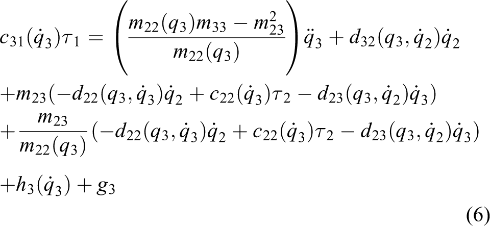
In the dynamics of the helicopter, as seen from equations (1) and (2), the ${\ddot{q}}_1\text{ and }{\ddot{q}}_2$ are coupled, which greatly increase the difficulty of the control design based on equation (1) directly. In order to simplify the system description and further develop controller for the helicopter, we decompose the systems (1) and (2) into three subsystems as follows

$\begin{array}{ll}\hfill & c_{11}({\dot{q}}_3){\tau }_1=m_{11}{\ddot{q}}_1+h_1({\dot{q}}_3)+g_1\hfill \end{array}$

4

$\begin{array}{ll}\hfill & c_{22}({\dot{q}}_3){\tau }_2=\left(\frac{m_{22}(q_3)m_{33}-m_{23}^2}{m_{33}}\right){\ddot{q}}_2+d_{23}(q_3,{\dot{q}}_2){\dot{q}}_3\hfill \\ \hfill & +d_{22}(q_3,{\dot{q}}_3){\dot{q}}_2+\frac{m_{23}}{m_{33}}\left(-d_{32}(q_3,{\dot{q}}_2){\dot{q}}_2-g_3-h_3({\dot{q}}_3)\right)\hfill \\ \hfill & +\frac{m_{23}}{m_{33}}{c}_{31}({\dot{q}}_3){\tau }_1\hfill \end{array}$

5

$\begin{array}{l}{c}_{31}({\dot{q}}_3){\tau }_1=\left(\frac{m_{22}(q_3)m_{33}-m_{23}^2}{m_{22}(q_3)}\right){\ddot{q}}_3+d_{32}(q_3,{\dot{q}}_2){\dot{q}}_2\\ +m_{23}(-d_{22}(q_3,{\dot{q}}_3){\dot{q}}_2+c_{22}({\dot{q}}_3){\tau }_2-d_{23}(q_3,{\dot{q}}_2){\dot{q}}_3)\\ +\frac{m_{23}}{m_{22}(q_3)}(-d_{22}(q_3,{\dot{q}}_3){\dot{q}}_2+c_{22}({\dot{q}}_3){\tau }_2-d_{23}(q_3,{\dot{q}}_2){\dot{q}}_3)\\ +h_3({\dot{q}}_3)+g_3\end{array}$

6

After the aforementioned manipulations, we can perform system analysis and develop controllers for the subsystems.

Preliminaries

Radical basis function

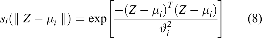
In this article, we use the RBFNNs to approximate an unknown continuous function $f(Z)$ as follows ⁷

$f_{nn}(Z)={\displaystyle \sum _{i=1}^N}{w}_i{s}_i(Z)=W^{T}S(Z)$

7

where $Z\in {\Omega }_Z\subset {ℝ}^m$ is the input vector, $W^T\in {ℝ}^N$ is the vector of NN weight, N is the number of NN nodes, $S(Z)=[s_1,s_2,\dots ,s_N{]}^T$ is the regressor vector, and $s_i(\cdot )$ is an RBF. The most commonly used Gaussian RBFs are implemented as follows

$s_i(\parallel Z-{\mu }_i\parallel )=\exp \left[\frac{-{(Z-{\mu }_i)}^T(Z-{\mu }_i)}{{\vartheta }_i^2}\right]$

8

and ${\mu }_i(i=1,\dots ,N)$ are distinct points with ${\mu }_i=[{\mu }_{i1},{\mu }_{i2},\dots ,{\mu }_{iq}{]}^T$ being the receptive field center and ϑ_i is the width of the receptive field. It has been proven that with sufficiently large number of nodes, RBFNN (7) could approximate any continuous function $f(Z)$ with arbitrary accuracy over a compact set Ω_Z as

$f\left(Z\right)=W^{*T}S\left(Z\right)+\epsilon (Z),\hspace{1em}\forall Z\in {\Omega }_Z$

9

where W* is the ideal constant weight vector, and $\epsilon (Z)$ is the NN construction error. There exists an ideal weight vector W* such that $\left|\epsilon (Z)\right|<{\epsilon }^{*}$ with constant ${\epsilon }^{*}>0$ for all $Z\in {\Omega }_Z$ . W* represents the value of W that could minimize $|\epsilon (Z)|\forall Z\in {\Omega }_Z$ , that is

$W^{*}:=\text{arg}\underset{W\in {ℝ}^N}{{\displaystyle \text{min}}}\left\{\underset{Z\in {\Omega }_Z}{{\displaystyle \text{sup}}}\right|f(Z)-W^{T}S(Z)\left|\right\}$

10

Note that the ideal weight vector W* is only used for analytical purposes. For real applications, we use the estimation $\widehat{W}$ .

Spatially localized approximation

The spatially localized approximation (SLA) of a localized RBF means that for any bounded trajectory remaining in a compact set, an unknown continuous function $f(z)$ can be approximated by a limited number of RBFs and neural nodes in a local region close nearby the trajectory, ³⁸ that is

$f\left(z\right)=W_{\xi }^{*T}{S}_{\xi }\left(z\right)+{\epsilon }_{\xi }(Z)$

11

where $S_{\xi }(z)=[z_1,z_2,\dots ,z_{\xi }{]}^T\in {ℝ}_{N\xi },\text{ and }N\xi <N,p_i>\varsigma$ with ς is a small positive constant, ε_ξ is the construction error.

Lemma 1. (Partial PE condition)

Consider that the trajectory $z(t)$ is periodic or recurrent and remain in the compact set Ω, $z(t)$ is continuous and $\dot{z}(t)$ is assumed to be bounded, and the centers of the localized RBF $W_{\xi }^T{S}_{\xi }(z)$ placed on a regular lattice (which means that the centers of NN could cover the compact set Ω), then the subvector $S_{\xi }(z(t))$ satisfies the PE condition. ⁴⁰

Remark 1

For the adaptive control and identification of the nonlinear system, the satisfaction of PE condition could ensure the convergence of the estimated parameters, and we can then reuse them in the learning control system without readaptation. However, the priori verification of the PE condition is difficult for identification of the nonlinear system. Based on the result of partial PE condition given in the literature, ⁴⁰ the localized RBFNN can be applied in the learning system by utilizing its function approximation ability, linear-in-parameter form, spatially localized ability, and the satisfaction of PE condition. The “partial” PE condition also means that the NN input trajectory does not need to visit all the centers of the regular lattice PE condition that hold for $W{\xi }^T{S}_{\xi }(z)$ as long as $z(t)$ is periodic like and stays within the regular lattice.

Useful function and key lemma. Definition 1

Let us define a set of switching functions $v(\cdot )$ as

$v(z)={\displaystyle \prod _{i=1}^n}{u}_i(z_i)$

12

where

${\mu }_i(z_i)=\{\begin{array}{c}1\text{\hspace{1em}\hspace{1em}\hspace{1em}\hspace{1em}\hspace{1em}\hspace{1em}\hspace{1em}\hspace{1em}if\hspace{1em}}\left|z_i\right|<=r_{i1}\\ \frac{r_{i2}^2-z_i^2}{r_{i2}^2-r_{i1}^2}{e}^{{\left(\frac{z_i^2-r_{i1}^2}{\varpi (r_{i2}^2-r_{i1}^2)}\right)}^2}\text{\hspace{1em}if\hspace{1em}}{r}_{i1}>\left|z_i\right|\ge r_{i2}\\ 0\text{\hspace{1em}\hspace{1em}\hspace{1em}\hspace{1em}\hspace{1em}\hspace{1em}\hspace{1em}\hspace{1em}elsewhere}\end{array}$

13

where $z=[z_1,z_2,\dots ,z_n{]}^T,r_{i1},r_{i2}$ are positive constants satisfying that $r_{i1}>r_{i2}$ , and ϖ is a designed constant with $\varpi >0$ .

Lemma 2

The following inequality holds for any $\omega >0\text{ and }f\in ℝ$ ^25,37 :

$0\le \left|f\right|-f\text{tanh}\left(\frac{f}{\omega }\right)\le \kappa \omega$

14

where κ is a constant with $\kappa =0.2785$ (satisfying $\kappa =e^{-(\kappa +1)}$ ).

Controller design

Problem formulation

For a helicopter system with $q_1(t)\text{ and }{q}_2(t)$ being the altitude position and yaw angular, respectively, and $q_3(t)$ the main rotor angular, our control goal is to develop an adaptive NN controller to ensure that (i) the altitude position $q_1(t)$ and yaw angular $q_2(t)$ of the helicopter could track a predefined trajectories $q_{1d}\text{ and }{q}_{2d}$ , while ensuring the tracking errors fall into a small neighborhood around zero; (ii) guarantee the stability and boundedness of the rate of main rotor angular ${\dot{q}}_3(t)$ ; (iii) all the signals in the helicopter system remain GUUB.

Adaptive NN learning control design

To achieve the aforementioned control goals, we first defined the residual tracking errors for the helicopter subsystems as

$e_i=q_i-q_{id}$

$s_i={\dot{e}}_i+{\gamma }_i{e}_i$

15

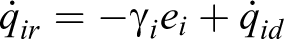
where γ_i is a selected positive constant, $i=1,2$ . In terms of the results in the study by Lewis et al., ⁴¹ if the filtering error s_i is bounded, we can obtain the boundedness of the tracking errors e_i and ${\dot{e}}_i$ . Then, the following auxiliary reference signals are designed as

${\dot{q}}_{ir}=-{\gamma }_i{e}_i+{\dot{q}}_{id}$

${\ddot{q}}_{ir}=-{\gamma }_i{\dot{e}}_i+{\ddot{q}}_{id}$

16

where ${\dot{q}}_{id}\text{ and }{\ddot{q}}_{id}$ are reference trajectories of the velocity and acceleration, respectively.

q₁ subsystem

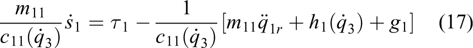
Using the definition of ${\dot{q}}_{1r},{\dot{q}}_{1r}$ , and s₁, the subsystem for ${\ddot{q}}_1$ can be rewritten as

$\frac{m_{11}}{c_{11}({\dot{q}}_3)}{\dot{s}}_1={\tau }_1-\frac{1}{c_{11}({\dot{q}}_3)}[m_{11}{\ddot{q}}_{1r}+h_1({\dot{q}}_3)+g_1]$

17

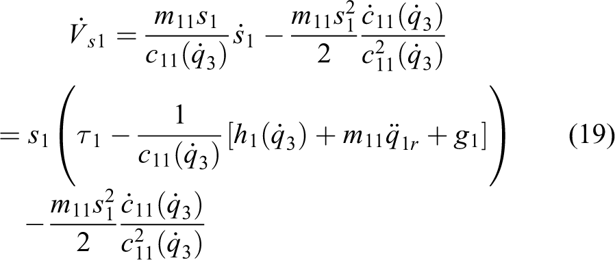
Then, let us consider the following Lyapunov function $V_{s_1}$ for the q₁ subsystem as

$V_{s_1}=\frac{m_{11}}{2c_{11}({\dot{q}}_3)}{s}_1^2$

18

Since the velocity of the main rotor ${\dot{q}}_3$ should satisfy ${\dot{q}}_3^2\ge g_0>0$ to overcome the gravity and lift the helicopter up, thus $c_{11}({\dot{q}}_3)=c_1{\dot{q}}_3^2>0$ , therefore $V_{s1}\ge 0$ is a Lyapunov candidate. Differentiate V _s1 with respect to time gives

$\begin{array}{c}{\dot{V}}_{s1}=\frac{m_{11}{s}_1}{c_{11}({\dot{q}}_3)}{\dot{s}}_1-\frac{m_{11}{s}_1^2}{2}\frac{{\dot{c}}_{11}({\dot{q}}_3)}{c_{11}^2({\dot{q}}_3)}\\ =s_1\left({\tau }_1-\frac{1}{c_{11}({\dot{q}}_3)}[h_1({\dot{q}}_3)+m_{11}{\ddot{q}}_{1r}+g_1]\right)\\ -\frac{m_{11}{s}_1^2}{2}\frac{{\dot{c}}_{11}({\dot{q}}_3)}{c_{11}^2({\dot{q}}_3)}\end{array}$

19

Let us define an auxiliary function f₁ for the V₁ as

$\begin{array}{c}{f}_1(z_1)=-\frac{1}{c_{11}({\dot{q}}_3)}(m_{11}{\ddot{q}}_{1r}+h_1({\dot{q}}_3)+g_1\\ +\frac{m_{11}{s}_1}{2}\frac{{\overline{c}}_{11}({\dot{q}}_3,{\ddot{q}}_3)}{c_{11}({\dot{q}}_3)})\end{array}$

20

where $z_1=[q_1,{\dot{q}}_1,q_{1d},{\dot{q}}_{1d},{\ddot{q}}_{1d},{\dot{q}}_3,{\ddot{q}}_3{]}^T\in {ℝ}^7\text{ and }{\overline{c}}_{11}({\dot{q}}_3,{\ddot{q}}_3)$ is a positive function with respect to ${\dot{q}}_3\text{ and }{\ddot{q}}_3$ and satisfies that $|{\dot{c}}_{11}({\dot{q}}_3)|\le {\overline{c}}_{11}({\dot{q}}_3,{\ddot{q}}_3)$ .

Substituting equation (20) into equation (19), we can rewrite equation (19) as

$\begin{array}{l}{\dot{V}}_{s1}=s_1({\tau }_1+f_1)-\frac{m_{11}{s}_1^2}{2c_{11}^2({\dot{q}}_3)}\left({\overline{c}}_{11}({\dot{q}}_3,{\ddot{q}}_3)+{\dot{c}}_{11}({\dot{q}}_3)\right)\hfill \end{array}$

21

In term of assumption 2, we find that

${\overline{c}}_{11}({\dot{q}}_3,{\ddot{q}}_3)+{\dot{c}}_{11}({\dot{q}}_3)>0$

22

The combination of equations (21) and (22) yields

${\dot{V}}_{s1}\le s_1({\tau }_1+f_1)$

23

Using the universal approximation property of RBFNN as mentioned in lemma 1, we can approximate the unknown function $f_1(z_1)$ by an RBFNN in the compact set Ω₁ as

$f_1(z_1)=W_1^{*}{}^T{S}_1(z_1)+{\epsilon }_1$

24

where $W_1^{*}\in {ℝ}^{L_1}$ is the optimal NN weight vector, L₁ is the number of NN nodes, $S_1(z_1)\in {ℝ}^{L_1}$ is the basis function vector, and ${\epsilon }_1\in ℝ$ is the NN construction error. It should be noted that $W_1^{*}$ is an unknown constant vector, and it would be estimated by ${\widehat{W}}_1$ , which is the estimation of $W_1^{*}$ .

Using the RBFNN control in equation (24), we can develop the global NN control input τ₁ for the q₁ subsystem as follows

${\tau }_1=-k_1{s}_1-v_1(z_1){\zeta }_{a1}-(1-v_1(z_1)){\zeta }_{b1}$

25

where k₁ is designed positive constant and $v_1(\cdot )$ is a switching function as defined in equation (13)

${\zeta }_{a1}={\widehat{f}}_1(z_1)={\widehat{W}}_1^T{S}_1(z_1)$

${\zeta }_{b1}=f_1^U\text{tanh}\left(\frac{s_1{f}_1^U(z_1)}{{\omega }_1}\right)$

26

where ${\widehat{f}}_1$ is the estimate of f₁, and we assume that f₁ is bounded by known nonnegative smooth function $f_1^U$ with $|f_1(z_1)|\le f^U(z_1)$ , and ω₁ is a positive parameter.

The NN weight adaptive law is designed as

${\dot{\widehat{W}}}_i=-{\Gamma }_1(s_1{v}_1(z_1)S_1(z_1)-{\sigma }_1{\widehat{W}}_1)$

27

where Γ₁ is a positive definitive matrix and σ₁ is a positive constant.

Remark 2

The controller proposed in equation (25) consists of an adaptive NN controller ${\zeta }_{a1}$ and an extra robust controller ${\zeta }_{b1}$ combining with a smooth switching function $v_1(z_1)$ . As seen from Figure 1, when the tracking runs in the NN active domain Ω₁, the term ${\zeta }_{a1}$ plays a decisive role, implying that the controller turns into a pure adaptive NN control. Once the NN runs out of the Ω₂, the extra robust term ${\zeta }_{b1}$ will take charge of the control and pull the state back to Ω₂. If the NN runs in the domain between the Ω₂ and Ω₁, the switching mechanism will work and pull the state to compact set Ω₁.

Figure 1.

Global tracking.

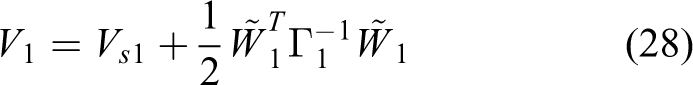
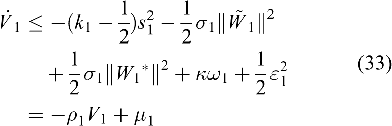
Then, let us consider the Lyapunov function V₁

$V_1=V_{s1}+\frac{1}{2}{\tilde{W}}_1^T{\Gamma }_1^{-1}{\tilde{W}}_1$

28

where ${\tilde{W}}_1=W_1^{*}-{\widehat{W}}_1$ . Differentiating equation (28) with respect to time, we have

${\dot{V}}_1\le s_1({\tau }_1+f_1)+{\tilde{W}}_1^T{\Gamma }_1^{-1}{\dot{\widehat{W}}}_1$

29

Substituting the control law (25) and the NN adaptive law (27) in equation (29), we have

${\dot{V}}_1\le -k_1{s}_1^2+s_1\left(-v_1(z_1){\zeta }_{a1}-(1-v_1(z_1)){\zeta }_{b1}+f_1\right)-{\tilde{W}}_1^T\left(s_1{v}_1(z_1)S_1(z_1)-{\sigma }_1{\widehat{W}}_1\right)\le -k_1{s}_1^2+s_1{v}_1(z_1)\left(f_1-{\widehat{W}}_1{S}_1(z_1)\right)+(1-v_1(z_1)\left(s_1{f}_1-s_1{f}_1^U\text{tanh}\left(\frac{s_1{f}_1^U(z_1)}{{\omega }_1}\right)\right)-{\tilde{W}}_1^T\left(s_1{v}_1(z_1)S_1(z_1)-{\sigma }_1{\widehat{W}}_1\right)\le -k_1{s}_1^2+v_1(z_1)s_1{\epsilon }_1+(1-v_1(z_1)\left(s_1{f}_1-s_1{f}_1^U\text{tanh}\left(\frac{s_1{f}_1^U(z_1)}{{\omega }_1}\right)\right)+{\sigma }_1{\tilde{W}}_1^T\left(W_1^{*}-{\tilde{W}}_1\right)$

30

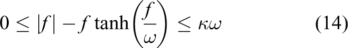
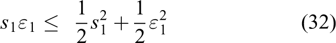
Note that the following inequalities holds in term of lemma 2

$\left|f_1^U{s}_1\right|-f_1^U{s}_1\text{tanh}\left(\frac{f_1^U{s}_1}{{\omega }_1}\right)\le \kappa {\omega }_1$

31

The following relation can be easily obtained according to the Young’s inequality

${\tilde{W}}_1{}^T(W_1^{*}-{\tilde{W}}_1)\le -\frac{1}{2}\left|\right|{\tilde{W}}_1{\left|\right|}^2+\frac{1}{2}\left|\right|W_1{}^{*}{\left|\right|}^2$

$s_1{\epsilon }_1\le \frac{1}{2}{s}_1^2+\frac{1}{2}{\epsilon }_1^2$

32

Substituting equations (31) and (32) into equation (30), we can deduce that

${\dot{V}}_1\le -(k_1-\frac{1}{2})s_1^2-\frac{1}{2}{\sigma }_1\Vert {\tilde{W}}_1{\Vert }^2+\frac{1}{2}{\sigma }_1\Vert W_1{}^{*}{\Vert }^2+\kappa {\omega }_1+\frac{1}{2}{\epsilon }_1^2=-{\rho }_1{V}_1+{\mu }_1$

33

where ${\rho }_1=\text{min}[\frac{(k_1-\frac{1}{2}){\overline{c}}_{11}}{m_{11}},\frac{{\sigma }_1}{{\lambda }_{\text{max}}({\Gamma }_1^{-1})}],{\mu }_1=\frac{1}{2}{\epsilon }_1^2+\frac{1}{2}{\sigma }_1\left|\right|W_1^{*}{\left|\right|}^2+\kappa {\omega }_1$ . Then, according to the Lyapunov theorem and in terms of equation (33), we can obtain that s₁ converges to a small residual set around zero by

${\Omega }_{s_1}=\left\{s_1:\left|s_1\right|\le \frac{{\mu }_1}{{\rho }_1}\right\}$

34

q₂ subsystem

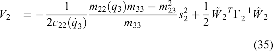
Considering the q₂ subsystem in equation (5), similar to the analysis of q₁ subsystem, let us define a Lyapunov candidate for the q₂ subsystem as

$\begin{array}{ll}{V}_2\hfill & =-\frac{1}{2c_{22}({\dot{q}}_3)}\frac{m_{22}(q_3)m_{33}-m_{23}^2}{m_{33}}{s}_2^2+\frac{1}{2}{\tilde{W}}_2{}^T{\Gamma }_2^{-1}{\tilde{W}}_2\hfill \end{array}$

35

According to property 3, and since $c_{22}({\dot{q}}_3)$ is negative, we can obtain that $V_2\ge 0$ is a valid Lyapunov candidate. Taking the deviation of equation (35) with respect to time, we have

${\dot{V}}_2=-\frac{d}{dt}\left(\frac{m_{22}(q_3)m_{33}-m_{23}^2}{m_{33}{c}_{22}({\dot{q}}_3)}\right)s_2^2+{\tilde{W}}_2{}^T{\Gamma }_2^{-1}{\dot{\widehat{W}}}_2-\frac{1}{c_{22}({\dot{q}}_3)}\frac{m_{22}(q_3)m_{33}-m_{33}^2}{m_{33}}{s}_2{\dot{s}}_2$

36

Using the definition of ${\dot{q}}_{1r},{\dot{q}}_{1r}$ , and s₁, we can obtain that ${\dot{q}}_2={\dot{q}}_{2r}+s_2,{\ddot{q}}_2={\ddot{q}}_{2r}+{\dot{s}}_2$ . Then, the q₂ subsystem can be rewritten as

$\begin{array}{ll}\hfill & -\left(\frac{m_{22}(q_3)m_{33}-m_{23}^2}{m_{33}}\right){\dot{s}}_2=\hfill \\ \hfill & -c_{22}({\dot{q}}_3){\tau }_2+\left(\frac{m_{22}(q_3)m_{33}-m_{23}^2}{m_{33}}\right){\ddot{q}}_{2r}+d_{22}(q_3,{\dot{q}}_3){\dot{q}}_{2r}\hfill \\ \hfill & +d_{23}(q_3,{\dot{q}}_2){\dot{q}}_3+\frac{m_{23}}{m_{33}}\left(-d_{32}(q_3,{\dot{q}}_2){\dot{q}}_2-g_3-h_3(\dot{q})\right)\hfill \\ \hfill & +d_{22}(q_3,{\dot{q}}_3)s_2+\frac{m_{23}}{m_{33}}{c}_{31}({\dot{q}}_3){\tau }_1\hfill \end{array}$

37

Substituting equation (37) into equation (36), we have

$\begin{array}{ll}{\dot{V}}_2\hfill & =-{\tau }_2{s}_2-\frac{d}{dt}\frac{m_{22}(q_3)m_{33}-m_{23}^2}{m_{33}{c}_{22}({\dot{q}}_3)}{s}_2^2+{\tilde{W}}_2{}^T{\Gamma }_2^{-1}{\dot{\widehat{W}}}_2\hfill \\ \hfill & +\frac{1}{c_{22}({\dot{q}}_3)}\left(\frac{m_{22}(q_3)m_{33}-m_{23}^2}{m_{33}}\right){\ddot{q}}_{2r}{s}_2\hfill \\ \hfill & +\frac{1}{c_{22}({\dot{q}}_3)}{s}_2\left(d_{23}(q_3\mathrm{,}{\dot{q}}_2){\dot{q}}_3+d_{22}(q_3\mathrm{,}{\dot{q}}_3){\dot{q}}_{2r}\right)\hfill \\ \hfill & +\frac{1}{c_{22}({\dot{q}}_3)}\frac{m_{23}}{m_{33}}{s}_2\left(-d_{32}(q_3\mathrm{,}{\dot{q}}_2){\dot{q}}_2-g_3-h_3(\dot{q})\right)\hfill \\ \hfill & +s_2\frac{1}{c_{22}({\dot{q}}_3)}\left(d_{22}(q_3\mathrm{,}{\dot{q}}_3)s_2+\frac{m_{23}}{m_{33}}{c}_{31}({\dot{q}}_3){\tau }_1\right)\hfill \end{array}$

38

Let us design an auxiliary function $f_2(z_2)$ as follows

$\begin{array}{l}{f}_2(z_2)=\frac{1}{c_{22}({\dot{q}}_3)}(\frac{m_{22}(q_3)c_{33}-m_{23}^2}{m_{33}}{\ddot{q}}_{2r}+d_{22}(q_3,{\dot{q}}_3){\dot{q}}_{2r}\hfill \\ \hspace{1em}\hspace{1em}+\frac{m_{23}}{m_{33}}(c_{31}({\dot{q}}_3){\tau }_1+d_{23}(q_3,{\dot{q}}_3){\dot{q}}_3-d_{32}(q_3,{\dot{q}}_2){\dot{q}}_2\hfill \\ \hspace{1em}\hspace{1em}-g_3-h_3({\dot{q}}_3))+\frac{1}{2}{s}_2^2\frac{m_{22}(q_3)m_{33}-m_{23}^2}{m_{33}}\frac{{\overline{c}}_{22}({\dot{q}}_3,{\ddot{q}}_3)}{c_{22}({\dot{q}}_3)})\hfill \end{array}$

39

where $z_2=[{\tau }_1,q_2,{\dot{q}}_2,q_{2d},{\dot{q}}_{2d},{\ddot{q}}_{2d},q_3,{\dot{q}}_3,{\ddot{q}}_3{]}^T$ . Note that the following inequality exists in term of assumption 2

${\overline{c}}_{22}({\dot{q}}_3,{\ddot{q}}_3)+{\dot{c}}_{22}({\dot{q}}_3)>0$

40

Then, substituting equations (39) and (40) into equation (38), and using property 3, we can obtain that

$V_2\le -s_2({\tau }_2-f_2)+\frac{1}{2}{\tilde{W}}_1^T{\Gamma }_1^{-1}{\tilde{W}}_1$

41

Using the approximation ability of RBFNN, the unknown system dynamics $f_2(z_2)$ can be formulated as

$f_2(z_2)=W_2^{*T}{S}_2(z_2)+{\epsilon }_2$

42

where $W_2^{*}\in {ℝ}^{L_2}$ is the optimal NN weight vector, L₂ is the number of NN nodes, $S_2(z_2)\in {ℝ}^{L_2}$ is the basis function vector, and ${\epsilon }_2\in ℝ$ is the NN construction error.

Then, the global NN controller for q₂ subsystem is designed as follows

${\tau }_2=k_2{r}_2+v_2(z_2){\zeta }_{2a}+(1-v_2(z_2)){\zeta }_{2b}$

43

where k₂ is a selected positive gain, and $v_2(\cdot )$ has been defined in equation (13)

${\zeta }_{a2}={\widehat{f}}_2(z_2)={\widehat{W}}_2^T{S}_2(z_2)$

${\zeta }_{b2}=f_2^U\text{tanh}\left(\frac{s_2{f}_2^U(z_2)}{{\omega }_2}\right)$

44

where ${\widehat{f}}_2$ is the estimate of f₂, and f₂ is bounded by known nonnegative smooth function $f_2^U$ with $|f_2(z_2)|\le f^U(z_2)$ , ω₂ is a positive parameter.

The NN weight adaptive law is designed as

${\dot{\widehat{W}}}_2=-{\Gamma }_2(s_2{v}_2(z_2)S_2(z_2)-{\sigma }_2{\widehat{W}}_2)$

45

where Γ₁ is a positive definitive matrix and σ₁ is a positive constant.

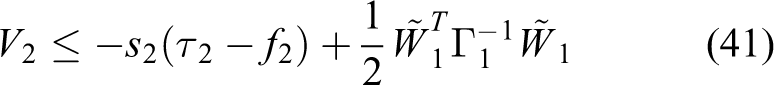
Substituting equations (43) to (45) into equation (41), and similar to the analysis in subsection “Problem formulation,” we can obtain that

${\dot{V}}_2\le -{\rho }_2{V}_2+{\mu }_2$

46

where ${\rho }_1=\text{min}[(k_2-\frac{1}{2}),(\frac{{\sigma }_2}{{\lambda }_{\text{max}}({\Gamma }_2^{-1})})],{\mu }_2=\frac{1}{2}{\epsilon }_2^2+\frac{1}{2}{\sigma }_2\left|\right|W_2^{*}{\left|\right|}^2+\kappa {\omega }_2$ . Then, according to the Lyapunov theorem, we can obtain that s₂ converges to a small residual set around zero by

${\Omega }_{s_2}=\left\{s_2:\left|s_2\right|\le \frac{{\mu }_2}{{\rho }_2}\right\}$

47

q₃ subsystem

In this subsection, we will investigate the stability of q₃ subsystem. In practice, the velocity of the main rotor ${\dot{q}}_3$ should satisfy ${\dot{q}}_3^2\ge g_0>0$ to overcome the gravity and lift the helicopter up. From systems (4) to (6) with control laws (25) and (43), we can rewrite q₃ subsystem as follows

$\dot{\eta }=f(\eta ,u,\xi ,)$

48

where $\eta =[q_3,{\dot{q}}_3{]}^T,u=[{\tau }_1,{\tau }_2{]}^T,\text{ and }\xi =[q_1,{\dot{q}}_1,q_2,{\dot{q}}_2{]}^T$ . Then, the zero dynamics of equation (48) can be obtained as

$\dot{\eta }=f(\eta ,u^{\ast }(0,\eta )\mathrm{,0})$

49

with $u^{*}=[{\tau }_1^{*},{\tau }_2^{*}]$ . Assume that system (48) is hyperbolically minimum phase, which means that the system zero dynamics (49) is exponentially stable. We also employ the assumption that the reference signals are all bounded and u is the control input with respect to ξ and η. Assume that the function $f(\xi ,\eta ,u)$ satisfies that

$\left|\right|f(\xi ,\eta ,u)-f(0,\eta ,u^{\ast }(0,\eta ))\left|\right|\le P_{\xi }\left|\right|\xi \left|\right|+P_f$

50

where P_ξ and P_f are constants. Then, the stability of q₃ subsystem is hold according to the following lemma.

Lemma 3

For the system $\dot{\eta }=f(\xi ,\eta ,u)$ as defined in equation (48), under assumptions 1 and 2, there exist positive constants P_η and T₀, such that ¹²

$\left|\right|\eta (t)\left|\right|\le L_{\eta },\forall t>T_0$

51

Stability analysis

Theorem 1

Consider the subsystems of helicopter dynamic in (4) (5) (6) with the tracking errors (15) under assumptions 1 and 2, employ the global NN controllers (25) and (43) with the NN weight adaptive laws in equations (27) and (45), then we have (i) all the signals remain GUUB and (ii) the tracking errors e₁ and e₂ converge to a small neighborhood of zero.

Proof

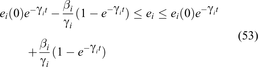
From the previous analysis, we find that ${\widehat{W}}_1,{\widehat{W}}_2$ , τ₁, and τ₂ are bounded and the filtered tracking errors s₁ and s₂ converge to a small compact set around zero, respectively. Then, substituting equation (15) into equations (33) and (46), we have

$-{\beta }_i\le {\dot{e}}_i+{\gamma }_i{e}_i\le {\beta }_{i}i=1,2$

52

where ${\beta }_i=\frac{{\mu }_i}{{\rho }_i}$ . The solution of the inequalities can be derived as follows

$\begin{array}{ll}\hfill & e_i(0)e^{-{\gamma }_{i}t}-\frac{{\beta }_i}{{\gamma }_i}(1-e^{-{\gamma }_{i}t})\le e_i\le e_i(0)e^{-{\gamma }_{i}t}\hfill \\ \hfill & +\frac{{\beta }_i}{{\gamma }_i}(1-e^{-{\gamma }_{i}t})\hfill \end{array}$

53

Then with $t\to \infty$ , we can obtain that

$\left|e_i\right|\le \frac{{\beta }_i}{{\gamma }_i}$

54

Then, let us investigate the boundedness of the closed-loop signals of the helicopter system. For the states variable q_i and ${\dot{q}}_i(i=1,2)$ , since e_i is bound, and $q_{id}\text{ and }{\dot{q}}_{id}$ are bounded in terms of assumption 1, we find that q₁, ${\dot{q}}_1$ , q₂, and ${\dot{q}}_2$ are bounded. Then, the boundedness of q₃ and ${\dot{q}}_3$ can be obtained in terms of lemma 3. Hence, we can deduce that all the closed-loop signals of the system are GUUB. In addition, the tracking errors e₁ and e₂ are also bounded by appropriately choosing the control gains k₁, k₂, γ₁, and γ₂. This completes the proof.

Remark 3

The designed control gains k₁ and k₂ in the controller should be chosen simply as positive constants, satisfying that $k_1>\frac{1}{2}\text{ and }{k}_2>\frac{1}{2}$ , while λ₁ and λ₂ should be chosen as positive constants. The gains in the NN adaptive laws Γ₁ and Γ₂ should be positive. If the gains k₁, k₂, Γ₁, and Γ₂ are chosen to be relatively large, while the σ₁ and σ₂ chosen to be relatively small, then the amplitude of tracking error could be made smaller.

Knowledge-reused NN control design

In this section, we will show that the adaptive NN controllers (25) and (43) with NN weight adaptations (27) and (45) are able to achieve knowledge expression, acquisition, and storage of uncertain system dynamics f₁ and f₂ in the steady-state control process. Then, the learned constant NN weights can be reused in the design of neural learning control to improve the control performance.

To achieve an accurate estimation of the converged NN weight, we will show that the inputs of NN, $W_1^T{S}_1,W_2^T{S}_2$ , are recurrent orbit. According to Theorem 1, we have shown that tracking error $e_i(i=1,2)$ converges to a small neighborhood around zero. Since $e_i=q_i-q_{id}$ and q_id is a recurrent orbit, thus q_i is recurrent orbit. It has also been proven that the filtered error s_i falls into a small neighborhood of zero, and γ_i is a bounded parameter; from equation (15), we know that ${\dot{q}}_i$ is also recurrent orbit. Therefore, the input of RBFNN, $W_i^T{S}_i$ , is the recurrent signal and the regressor subvectors, $S_{i\xi }(z_i)$ , satisfy the PE condition. Then, the results of NN learning ability can be formulated by the theorem below.

Theorem 2

Considering the helicopter system defined in equations (4) to (6), the filtered tracking errors in equation (15), and the NN adaptation law (27) and (45), for any recurrent orbit φ_i, and initial conditions ${\widehat{W}}_i(0)=0$ , we have that the NN weight estimate converges to small neighborhoods of its optimal value $W_i^{*}$ along ${\phi }_i{(z_i(t))}_{(t\ge T_i)}$ , and the system dynamics $f_i(z_i)$ could be approximated accurately by either ${\widehat{W}}_i^T{S}_i(z_i)$ or ${\overline{W}}_i^T{S}_i(z_i)$ to the desired error level ${\overline{\epsilon }}_i$ as

$f_i={\widehat{W}}_i^T{S}_i(z_i)+{\epsilon }_i(z_i)={\overline{W}}_i^T{S}_i(z_i)+{\overline{\epsilon }}_i(z_i)$

55

where ${\epsilon }_i(z_i)$ is close to ε_i in the steady-state process and ${\overline{W}}_i$ is defined as

${\overline{W}}_i=\frac{1}{t{c}_i-t{b}_i}{\displaystyle {\int }_{t{b}_i}^{t{c}_i}}{\widehat{W}}_i(r)dr$

56

where $t{c}_i>t{b}_i>T_1$ denotes the time segment in the steady stage.

Proof

According to Theorem 1, we have that in the steady stage, the system states q₁, q₂, ${\dot{q}}_1,{\dot{q}}_2$ and tracking errors q₁ and q₂ subsystems can converge to small compacts. Therefore, it is reasonable for us to employ the assumption that the inputs of the NN $W_1{S}_1\text{ and }{W}_2{S}_2$ would remain in a compact set after the transient stage. Hence, the NNs controller ${\zeta }_{a1}\text{ and }{\zeta }_{a2}$ are always valid at the steady stage, and the controller can be rewritten as follows

${\tau }_1=-k_1{s}_1-{\widehat{W}}_1^T{S}_1$

${\tau }_2=k_2{s}_2+{\widehat{W}}_2^T{S}_2$

57

Let us employ the SLA ability of RBFNNs with the controller (57), then the q₁ and q₂ subsystems could be rewritten as follows:

${\psi }_i{\dot{s}}_i=-k_i{s}_i-{\tilde{W}}_{i\xi }^T{S}_{i\xi }(z_i)+{\epsilon }_i$

${\dot{\tilde{W}}}_{i\xi }=-{\Gamma }_i(s_i{S}_{i\xi }(z_i)-{\sigma }_i{\widehat{W}}_{i\xi })$

58

where ${\psi }_1=\frac{c_{11}({\dot{q}}_3)}{m_{11}}\text{ and }{\psi }_2=-\frac{m_{33}{c}_{22}({\dot{q}}_3)}{m_{22}(q_3)m_{33}-m_{23}^2}$ . Since $c_{11}({\dot{q}}_3)$ , m₁₁, m₃₃, and $m_{22}(q_3)m_{33}-m_{23}^2$ are positive and $c_{22}({\dot{q}}_3)$ is negative, we can obtain that ψ₁ and ψ₂ are positive. By defining ${\dot{\varphi }}_{si}=\frac{s_i}{{\psi }_i}$ , equation (58) can be rewritten in linear time-varying form as

$\left[\begin{array}{c}{\dot{\varphi }}_{si}\\ {\dot{\tilde{W}}}_{i\xi }\end{array}\right]=\left[\begin{array}{cc}{A}_{11}(t)& S_{i\xi }^T(z_i)\\ A_{21}(t)& 0\end{array}\right]\left[\begin{array}{c}{\varphi }_{si}\\ {\tilde{W}}_{i\xi }\end{array}\right]+\left[\begin{array}{c}{\epsilon }_i\\ {\sigma }_i{\Gamma }_i{\widehat{W}}_{i\xi }\end{array}\right]$

59

where $A_{11}(t)=-k_i{\psi }_i-\frac{{\dot{\psi }}_i}{{\psi }_i}\text{ and }{A}_{21}=-{\Gamma }_i{\psi }_i{S}_i(z_i)$ . Let $P(t)={\psi }_i>0$ , we have $\dot{P}(t)+P(t)A_{11}(t)+A_{11}^T(t)P(t)=-2k_i{\psi }_i^2-{\dot{\psi }}_i$ .

Then, following the proof as in the work of Dai et al. ³⁸ and Wang and Hill, ⁴⁰ we can obtain that the NN weights estimate error ${\tilde{W}}_{i\xi }$ could exponentially converge to zero. Therefore, ${\widehat{W}}_i$ can converge to a small neighborhood nearby the optimal NN weight $W_i^{*}$ . This completes the proof.□

Then, we can reuse the constant weight of RBFNN $W_i{S}_i(z_i)$ to reconstruct the static NN controller to achieve the improvement of control of the helicopter system when tracking a similar trajectory. The NN controller with learned knowledge is designed using the constant NN weight and without the NN weight updated law as

$\begin{array}{ll}{\tau }_1\hfill & =-k_1{s}_1-v_1(z_1){\overline{\zeta }}_{a1}-(1-v_1(z_1)){\zeta }_{b1}\hfill \\ {\tau }_2\hfill & =k_2{s}_2+v_2(z_2){\overline{\zeta }}_{a2}+(1-v_2(z_2)){\zeta }_{b2}\hfill \end{array}$

60

where ${\overline{\zeta }}_{a1}={\overline{W}}_1^T{S}_1\text{ and }{\overline{\zeta }}_{a2}={\overline{W}}_2^T{S}_2$ . W₁ and W₂ are the constant NN weight vectors that are obtained from equation (56).

Subsequently, we can apply the developed neural learning controller with the stored knowledge to control the helicopter with improved control performance.

Simulation studies

In this section, simulation studies are carried out to illustrate the effectiveness of the proposed global NN control algorithms (25) and (43). In the simulation, the helicopter dynamics and parameters are described using the Vario model ⁴²

$M(q)\ddot{q}+D(q,\dot{q})\dot{q}+H(\dot{q})+G(q)=C\tau$

61

with

$\begin{array}{ll}M(q)=\hfill & \left[\begin{array}{ccc}7.5& 0& 0\\ 0& m_{22}& 0.108\\ 0& 0.108& 0.4993\end{array}\right]\hfill \\ D(q,\dot{q})=\hfill & \left[\begin{array}{ccc}0& 0& 00\\ d_{22}& d_{23}& \\ 0& d_{32}& 0\end{array}\right]\hfill \\ H(\dot{q})=\hfill & \left[\begin{array}{c}-0.60{\dot{q}}_3\\ 0\\ -0.0001206{\dot{q}}_3^2\end{array}\right]\hfill \\ C(\dot{q})=\hfill & \left[\begin{array}{ccc}3.41{\dot{q}}_3^2& 0& \\ 0& -0.153{\dot{q}}_3^2& \\ 12.01{\dot{q}}_3+{10}^5& 0& \end{array}\right]\hfill \\ G(q)=\hfill & \left[\begin{array}{c}-77.259\\ 0\\ -2.642\end{array}\right]\hfill \end{array}$

62

with the term chosen to be $d_{22}=0.00062\text{sin}(-8.29q_3){\dot{q}}_3,d_{23}=d_{23}=0.00062\text{sin}(-8.29q_3){\dot{q}}_2,m_{22}=0.43+0.0003{{\displaystyle \cos }}^2(-4.143q_3)$ .

The helicopter is commanded to follow the reference trajectory as follows

$\begin{array}{l}{q}_{1d}=\{\begin{array}{cc}-0.2& 0\le t\le 6s\\ 0.1\cos (0.1(t-6))-0.3& 6<t\le 78s\end{array}\\ \\ q_{2d}=\{\begin{array}{cc}0t<6s\mathrm{,30}\le t<42,& 66\le t<78\\ 1-\text{exp}(-{(t-6)}^2/50)& 6\le t<12s\\ 0.5112\le t<24s& 48\le t<60s\\ \text{exp}(-{(t-24)}^2/50)-0.49& 24\le t<30\\ 1-\text{exp}(-{(t-42)}^2/50)& 42\le t<48s\\ \text{exp}(-{(t-60)}^2/50)-0.49& 60\le t<66\end{array}\end{array}$

63

In terms of the zero dynamics as mentioned in section “q ₃ subsystem”, let s₁, s₂, ${\tilde{W}}_1^T,{\tilde{W}}_2^T,{\epsilon }_1^T,\text{ and }{\epsilon }_2^T$ are all zero, and the desired trajectories can be obtained as

${\ddot{q}}_3=\frac{1}{m_{33}}\left[\frac{c_{31}(\dot{q})}{c_{11}(\dot{q})}(m_1(\dot{q})+g_1)-h_3(\dot{q})-g_3\right]$

64

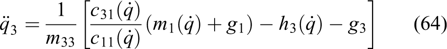
By linearizing equation (64) and substituting equation (62) into equation (64), and using the assumption that the acceleration of angular is zero, we can obtain that the equilibrium point of dynamics equation is close to ${\dot{q}}_3^{*}=-124$ and its eigenvalue is negative, which demonstrate that the helicopter dynamics has observed a stable behavior.

For the global NN control laws and adaptation laws with the input vectors $z_1=[q_1,{\dot{q}}_1,{\dot{q}}_3,{\ddot{q}}_3,q_{1d},{\dot{q}}_{1d},{\ddot{q}}_{1d}],z_2=[{\tau }_1,q_2,{\dot{q}}_2,{\dot{q}}_{2d},{\ddot{q}}_{2d},q_{2d},q_3,{\dot{q}}_3,{\ddot{q}}_3{]}^T$ , we employ totally 2187 nodes for $W_1{S}_1(z_1)$ and 19,683 nodes for $W_2{S}_2(z_2)$ , the centers of S₁ are evenly spaced in, $[-1.05,1.05]\times [-0.1,0.1]\times [-100.0,-50.0]\times [-30.0,30.0]\times [-1.05,1.05]\times [-0.1,0.1]\times [-0.01,0.01]$ and centers of S₂ are evenly spaced in $[-0.005,0.005]\times [-10.0,10.0]\times [-40000,0.0]\times [-10.0,10.0]\times [-1.05,1.05]\times [-0.01,0.01]\times [-1.05,1.05]\times [-100.0,-50.0]\times [-20.0,50.0]$ , respectively. The widths are chosen as ${\vartheta }_1=1\text{ and }{\vartheta }_2=1$ . The control gains and design parameters are selected to be $k_1=1.0,k_2=1.0,{\gamma }_1=1.0,\text{ and }{\gamma }_2=1.0$ . The initial states are set as $q_1(0)=-0.15,q_2(0)=-\pi ,q_3(0)=-\pi ,{\dot{q}}_1(0)=0\text{ and }{\dot{q}}_2(0)=0,{\dot{q}}_3(0)=-120,{\widehat{W}}_1(0)=0,{\widehat{W}}_2(0)=0$ .

The simulation results are shown in Figures 2 to 7.

Figure 2.

Tracking performance of q ₁.

Figure 3.

Tracking performance of q ₂.

Figure 4.

Tracking errors e ₁.

Figure 5.

Tracking errors e ₂.

Figure 6.

Control input τ ₁.

Figure 7.

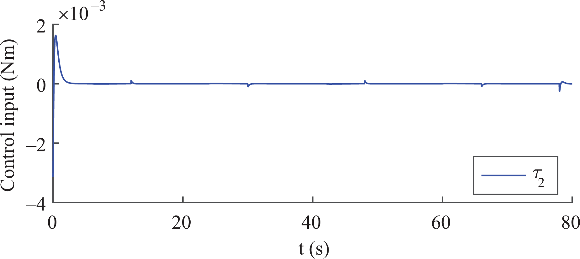
Control input τ ₂.

The tracking performance of the helicopter attitude position q₁ and the yaw angle q₂ is depicted in Figures 2 and 3.

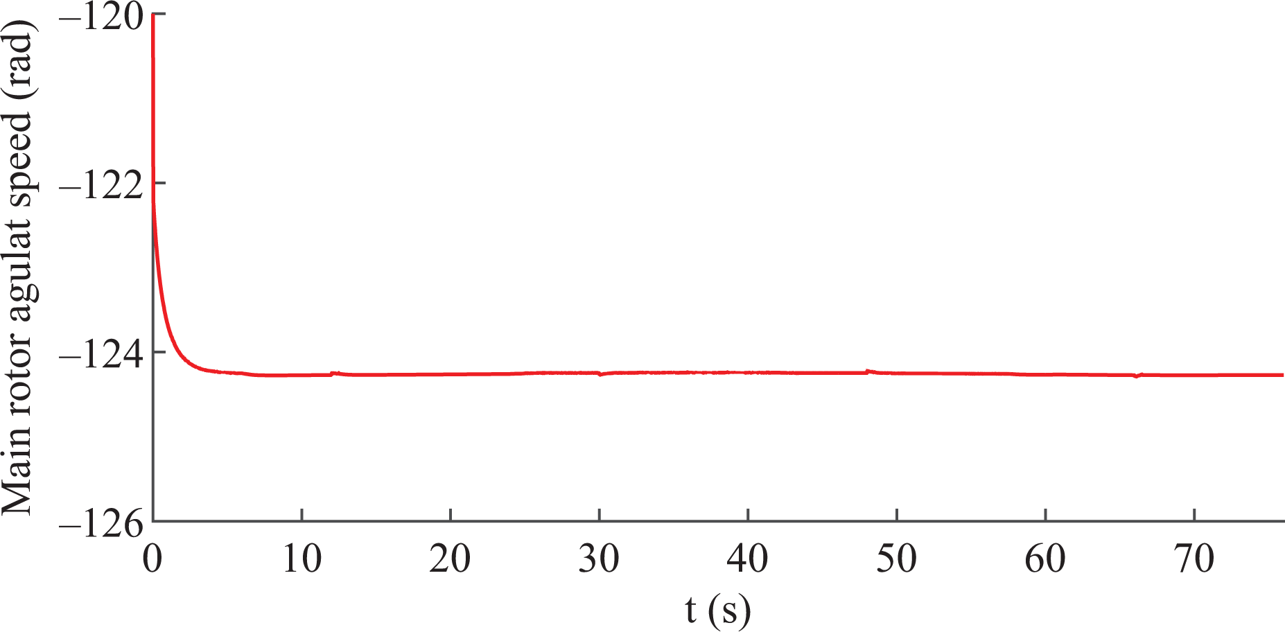
We see clearly that q₁, q₂, ${\dot{q}}_1,\text{ and }{\dot{q}}_2$ could effectively follow the reference trajectories with a good steady-state performance. This implies that the proposed controller can achieve a good tracking performance in the presence of unknown dynamics. The performance of tracking errors e₁ and e₂ is shown in Figures 4 and 5. As shown in the figures, using the proposed global RBFNN controller, the tracking errors converge to a small value close to zero with fast converge rate and good steady-state performance. A comparative simulation study is performed based on a model-based controller. From Figures 4 and 5, we can see that the proposed RBFNN controller is better than the model-based controller. Additionally, Figure 8 indicates that the speed of the main rotor angular is stable. Figures 6 and 7 illustrate that the control inputs τ₁ and τ₂ are bounded. The simulation results illustrate that our proposed global RBFNN controller can ensure the helicopter to effectively track a predefined trajectory and guarantee the tracking error converge to a small neighborhood near zero.

Figure 8.

Main rotor angular speed . ${\dot{q}}_3$

Conclusion

This article investigates the NN control for an unmanned helicopter in the presence of unknown system dynamics. NN control is constructed to compensate the unknown dynamics of each subsystem of the helicopter. A switching mechanism is also integrated into the control design to extend the SGUUB to GUUB, such that the resulted neural controller is always valid without any concern on either initial conditions or range of state variables. Deterministic learning technique is applied to improve control performance, with the storage of the learned knowledge of the adaptive neural learning control. Simulation studies have shown the validity and effectiveness of proposed control design based on the helicopter models.