Sage Journals: Discover world-class research

Abstract

This article presents implementation of an online gait generator on a quadruped robot. Firstly, the design of a quadruped robot is presented. The robot contains four leg modules each of which is constructed by a 2 degrees of freedom (2-DOF) five-bar parallel linkage mechanism. Together with other two rotational DOF, the leg module is able to perform 4-DOF movement. The parallel mechanism of the robot allows all the servos attached on the body frame, so that the leg mass is decreased and motor load can be balanced. Secondly, an online gait generator based on dynamic movement primitives for the walking control is presented. Dynamic movement primitives provide an approach to generate periodic trajectories and they can be modulated in real time, which makes the online adjustment of walking gaits possible. This gait controller is tested by the quadruped robot in regulating walking speed, switching between forward\backward movements and steering. The controller is easy to apply, expand and is quite effective on phase coordination and online trajectory modulation. Results of simulated experiments are presented.

Keywords

Quadruped robot parallel linkage mechanism modular structure motor primitives moving control

Introduction

Quadruped robots are useful in many tasks due to their ability to walk smoothly on rough terrain.¹ Among many research interests regarding the quadruped robot, the system design and the control of walking have long been key issues. Traditional motion control method can be interpreted as a kind of feed forward control strategy. Most of them^2
–4 need information of the terrain no matter from a known map or sensor detection. The motion controller tries to compensate the disturbance before it can make any effects on the system. Feed forward control needs an accurate and complicated model. As we can see in Estremera’s research,³ it requires different kinds of predefined stability margins, different kinds of techniques such as query, searching and optimization. So same drawbacks as a feed forward control strategy have, traditional motion planning generally consumes much time, and is too complicated to extend or transplant. On the other hand, these characteristics make this approach quite suitable for low-speed discontinuous static gait generating which allows the robot to stop and think and avoid leg coordination at the same time. In this situation, the robot using traditional motion planning can also have the ability to move Omnidirectionally.

Another way is based on biologically inspired strategy. It is actually a feedback control strategy with a dynamic system as its controller. Typically, a controller does algebraic operation on state variables of the controlled object. While choosing a dynamic system as a controller makes controlling more like an interaction between the controlled object and the dynamic system consisting the controller and introduces more state variables. Most popular biologically inspired strategy is central pattern generator⁵ (CPG). A typical approach to express CPG is to design an autonomous dynamic system of coupled non-linear oscillators. This autonomous dynamic system can be a network⁶ or just two coupled oscillators,⁷ and its working space can also be different, either joint space^7,8 which means the output signal of CPG is interpreted as a joint angle signal or leg coordination Cartesian space.^6,9 A significant advantage of CPG is that it can be easily extended and is able to reject the real-time disturbances.^10
–12

CPG is easy to extend as its structure is quite simple but not easy to design as it’s a non-linear dynamic system. Because the curve of output signal of most CPGs cannot be arbitrarily reshaped, there comes the need for designing a CPG that can predefine the output curve. Dynamical movement primitives (DMPs)^13
–15 provides a good solution for this problem. Meanwhile it keeps the advantages of typical CPGs like the relative simple structure, disturbance robustness and coordination mechanism. The concept of primitives, motor primitives or movement primitives comes from biological research, which means basic elements that can generate complicate movements.¹⁶

In this article, we use DMP as a strategy to control a quadruped robot. A DMP-based controller is established to achieve movement, and the output signal is explained in leg coordination Cartesian space. The design of a quadruped robot is proposed to test the control method. The robot is made up of body frames and four leg modules (Figure 1). Together with other two rotation DOF, the leg module is able to perform 4-DOF movement. The parallel mechanism of the robot allows all the servos attached on the body frame, so that the leg mass is decreased and motor load can be balanced. As four leg modules attach under the trunk separately, control system and power system can be settled on the trunk without any collisions with the four leg modules. The simulation results show that the robot can do basic walking targets such as walking in a certain gait, speed control and turning control. Switches between different targets can be achieved naturally and smoothly.

Figure 1.

Design of a modular quadruped robot. Left: the modular quadruped robot. Right: structure of a leg module.

The article is organized as follows. The mechanical design of the robot is discussed in section ‘Design of the quadruped robot’. DMPs used to build gait controllers are introduced in section ‘Dynamical movement primitives’. In section ‘Proposed controller’, the online walking gait generator is discussed. Simulation results of the control method are presented in section ‘Simulation results and discussion’.

Design of the quadruped robot

We designed a robot actuated by 12 electrical servos. Although the power of an electric motor has been greatly improved, one still needs to carefully design the leg of a quadruped robot in order to reduce the leg mass and balance the payload of different motors. In order to reduce the energy consuming of motors, a leg module constructed by mixed serial/parallel mechanisms is proposed. The size of this modular robot is about 45 cm long, 30 cm high and 30 cm wide, without other systems carried on.

Design of the leg module

A leg module includes a base and a five-bar mechanism (Figure 1). Base is directly connected to the trunk, while the five-bar mechanism can rotate along the hip shaft. By adding four servos, we can control the free end moving within the plane constructed by five-bar mechanism, roll motion of the five-bar mechanism and the yaw motion of the whole module.

Servo 1 and servo 2 are responsible for the controlling of the five-bar mechanism. Servo 3 is responsible for the roll motion of the five-bar mechanism. It can control the rotate motion of five-bar mechanism along the hip shaft. Servo 4 is responsible for the controlling of the yaw motion of the whole module. With the control of these two servos, we can control the free end of the leg moving within the plane constructed by five-bar mechanism. Because this structure is a typical parallel mechanism, no servos here need to carry the other one. Besides, this design leaves the leg-only links, thus reduce the leg mass.

Kinematics of the five-bar mechanism

Before the analysis, we can simplify the five-bar mechanism into the diagram shown in Figure 2.

Figure 2.

Simplified five-bar mechanism. θ_i is joint angle and L_i is linkage length. This mechanism is exactly the same one used in left fore and right hind leg. While in left hind and right fore leg, the mechanism used is the mirror structure of the above one. Considering that the kinematics of the mirror structure is similar to the original one, we only talk about the original structure in this article.

There are different ways to calculate the forward and inverse kinematics, like using rotation matrix or vector equation and so on. Here, we decomposed this problem into a simple question, then both forward and backward kinematics are solved based on the reuse of this simple question. This method gets rid of the massive usage of trigonometric functions and is easy to program in a computer.

The simple question:

Given two different points: P ₁(x₁, y₁) and P ₂(x₂, y₂). Calculate the coordinates of point P so that its distance to P ₁ is l₁ to P ₂ is l₂. (Assume that P exists.)

Solution:

According to the question, we can get the equations below

{(x_{p} - x_{1})}^{2} + {(y_{p} - y_{1})}^{2} = l_{1}^{2}

{(x_{p} - x_{2})}^{2} + {(y_{p} - y_{2})}^{2} = l_{2}^{2}

Solutions of these two equations are

y_{p} = \frac{x_{2} \sqrt{A . B} - x_{1} \sqrt{A . B} + E}{F}

y_{p} = \frac{x_{1} \sqrt{A . B} - x_{2} \sqrt{A . B} + E}{F}

Where

A = {(l_{1} + l_{2})}^{2} - {(x_{1} - x_{2})}^{2} - {(y_{1} - y_{2})}^{2}

B = - {(l_{1} - l_{2})}^{2} + {(x_{1} - x_{2})}^{2} + {(y_{1} - y_{2})}^{2}

E = {(y_{1} - y_{2})}^{2} . (l_{2}^{2} - l_{1}^{2}) + (y_{1} + y_{2}) . [{(x_{1} - x_{2})}^{2} - y_{1} y_{2}] + y_{1}^{3} + y_{2}^{3}

F = 2 [{(x_{1} - x_{2})}^{2} + {(y_{1} - y_{2})}^{2}]

Then x_p can be calculated by

x_{p} = ± \sqrt{l_{1}^{2} - {(y_{p} - y_{1})}^{2}} + x_{1}

There are at most two P points and one of the x_p in equation (5) should be regarded. One can easily check this through equation (2), so that all the right two P points can be found.

The forward kinematics can be calculated following the procedures below:

Step 1. Calculate the coordinates of point B and D (Figure 2).

Step 2. As the distances between C and B and C and D keep constant, one can use the solutions of the simple question to calculate C. Choose the one with bigger y coordinate.

Step 3. As the distances between P and C and P and D keep constant, one can use the solutions of the simple question to calculate P. Choose the one with bigger y coordinate. (One can also rotate CD to get the coordinate of P.)

The inverse kinematics can be calculate following the procedures below:

Step 1. As the distances between D and P and D and E keep constant, one can use the solutions of the simple question to calculate D. Choose the one with bigger x coordinate.

Step 2. As the distances between C and D and C and P keep constant, one can use the solutions of the simple question to calculate C. Choose the one with smaller y coordinate (or using rotation matrix).

Step 3. As the distances between B and C and B and A keep constant, one can use the solutions of the simple question to calculate B. Choose the one with smaller x coordinate.

Step 4. Calculate the servo angle through the coordinates of point D and B.

Generally, in the inverse kinematics, there are four possible solutions. The choice of D can be the one with smaller x coordinate instead of the bigger one, so as to the choice of B. One can see this more clearly in Figure 3. Since this five-bar structure can be seen as the combination of two typical second-order serial leg: AB-BC and ED-DCP, it inherits the problem of multi-solution of a second-order serial leg. Here, we choose the solution that makes ABCDE a convex polygon as the final solution.

Figure 3.

Four solutions of the inverse kinematics of the same foot end.

Dynamical movement primitives

DMPs are originally proposed by Ijspeert et al.,¹⁴ while a simple review of DMP is presented here in this section since it’s the basis of our control strategy. DMP is a line of research for modelling attractor behaviours of autonomous non-linear dynamic system with the help of statistical learning techniques.¹⁴ Both point and limit cycle attractor are included but only the last one is introduced here, as we only need periodic motions.

Basic structure of DMP

A DMP can be divided into three parts: canonical system, forcing term and transformation system. The former’s output will be the latter’s input, making the whole DMP like a cascade system. So we can conclude the three parts’ equations as follows

\dot{ϕ} = C

f = p_{1} (ϕ)

y = p_{2} (f, ż, ẏ)

In these equations, equation (6) stands for canonical system, equation (7) stands for forcing term and equation (8) stands for transformation system, where y and z in equation (8) are the state variables. Actually, equation (6) is a proportional function with output regulated into [0,2π] (see equation (9)), which makes the canonical system a periodic phase oscillator

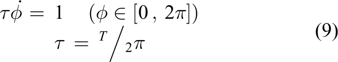
\begin{array}{l} τ \dot{ϕ} = 1 (ϕ \in [0, 2 π]) \\ τ = \frac{T}{2 π} \end{array}

Where T is the period of the learned trajectory. The parameter τ makes the periods of canonical system and learned trajectory stay the same. Forcing term will drive the transformation system to reach the trajectory we want. Its equation (7) is a set of algebraic equations, which is the only non-linear part of DMP

f (ϕ) = p_{1} (ϕ) = \frac{\sum_{i = 1}^{N} ψ_{i} ω_{i}}{\sum_{i = 1}^{N} ψ_{i}} r

ψ_{i} = \exp (h_{i} (\cos (ϕ - c_{i}) - 1))

Where the exponential basis functions in equation (11) are fixed von Mises basis functions, essentially Gaussian-like functions. ω are adjustable weights, r is a scale factor which does not change during online calculation here. Representing arbitrary non-linear functions as such, a normalized linear combination of basis functions has been a well-established methodology in machine learning or statistical learning techniques, which means we can arbitrarily change the shape of this forcing term’s output. So finally we can arbitrarily change the output of the whole DMP.

Transformation system can be seen as a low-pass filter for forcing term, and here it is a linear time-invariant system modelled from spring-damping system

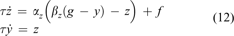
\begin{array}{l} τ ż = α_{z}^{} (β_{z} (g - y) - z) + f \\ τ ẏ = z \end{array}

If the forcing term f = 0, these equations represents a globally stable second-order linear system with (z, y) = (0, g) as a unique point attractor. With appropriate values of α_z and β_z, the system can be made critically damped in order for y to monotonically converge towards g. Another advantage of a linear time-invariant system is that it can be discretized easily without precision lost instead of using numeric methods to solve these differential equations. As to the whole DMP, the only non-linear part is algebraic equations, so we can get its discretization model without any precision lost.

When the form of the transformation system is known, it’s easy to make DMP output the desired trajectory. According to equation (12), we can get

f_{d} = τ^{2} ÿ_{d} + τ α_{z} ẏ_{d} + α_{z} β_{z} (y_{d} - g)

Where y_d is the desired or pre-defined trajectory. Through equation (13), the desired f trajectory can be calculated from the desired output trajectory. Then by using the machine learning or statistical learning techniques, the adjustable weight ω can be calculated. So the whole DMP can work by calculating equations (6) to (8) successively.

Amplitude and frequency scale

Amplitude and frequency scale can be solved in the framework of topological equivalence. The results are very simple. Assume the frequency scale factor is K_f and the amplitude is K_A, then the amplitude scale law is

y \to K_{A} y ẏ \to K_{A} ẏ z \to K_{A} z ż \to K_{A} ż

The frequency scale law is

ż \to \frac{ż}{K_{f}} ẏ \to \frac{ẏ}{K_{f}} \dot{ϕ} \to \frac{ϕ}{K_{f}}

Where the notation → denotes a functional mapping, z and y are state variables in transformation system, Φ is the output of the canonical system.

Coordination between different DMPs

The coordination between different DMPs is achieved by coordinating the different belonging canonical systems. A canonical system can be seen as the power supplier of a DMP and it is essentially a phase oscillator, so synchronization theory can be used.¹⁷ For general coordinating between two oscillators, there are three different ways: frequency lock, phase lock and injection lock. Injection lock can achieve frequency lock and phase lock at the same time. It is chosen here to lock two DMPs. Modified canonical system is shown in equation (16)

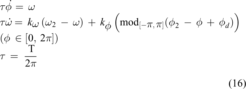
\begin{array}{l} τ \dot{ϕ} = ω \\ τ \dot{ω} = k_{ω} (ω_{2} - ω) + k_{ϕ} (\mod_{[- π, π]} (ϕ_{2} - ϕ + ϕ_{d})) \\ (ϕ \in [0, 2 π]) \\ τ = \frac{T}{2 π} \end{array}

Where ϕ_d is the desired phase difference, ω₂ and ϕ₂ come from another oscillator and k_ω and k_ϕ are positive parameters. Comparing with equation (9), there actually adds a PID controller to canonical system with ϕ_d as its reference.

Proposed controller

This section introduces the controller we designed for quadruped walking by using DMP as its core. The actuators we used are servo motors, so the output of our controller is position information.

Predesign trajectory

In our work, we only use two main coordinates to observe the motion of the quadruped: the body coordinate frame Σ_b attached to the centre of the robot and the global coordinate frame Σ_g attached to the ground. Since we only considered open loop control so far, global coordinate frame is only used in experiment observation. The predesign trajectory of the foot is considered in Σ_b.

The trajectory is designed in YZ plane in Σ_b or the so-called sagittal plane. Its shape is shown in Figure 4. Since we want the robot to keep its height unchanged when this foot touches the ground and considering our gait is actually a kind of static period gait, making bottom a horizontal line is straightforward.

Figure 4.

Left graph is the predesign trajectory in sagittal plane. Right graph is decomposition of y and z direction. Remind that the origin of this graph is not the origin of YZ or sagittal plane. We define a new origin here just to make it easier to generate such a predesign trajectory.

The parameters of this trajectory include: period T, the lasting time of vertical segment T_v, the length of vertical segment L_v and the step time d_t. We generate this trajectory by using difference equations, which makes it easy to implement through numeric methods, avoid large changes and be decomposed to YZ direction during generating (see Figure 4). But the drawback of this approach is also obvious: the begin point and the end point are hard to meet. Fortunately, due to the low-pass characteristic of DMP, this drawback can be easily avoided.

Figure 5 shows the output through DMP. The result is actually combined by two DMPs with one generating z direction trajectory and the other one generating y direction. We set the initial output of DMP is the mechanical zero point which is different from the trajectory point, but we can see that DMP makes a smooth transportation due to its low-pass characteristic.

Figure 5.

Output through DMP. Due to the low-pass characteristic of DMP, the trajectory goes through the beginning and last point smoothly. Even though the start point isn’t at the trajectory’s beginning point, DMP can create a smooth transportation. DMP: dynamic movement primitive.

Single leg module and the overall controller

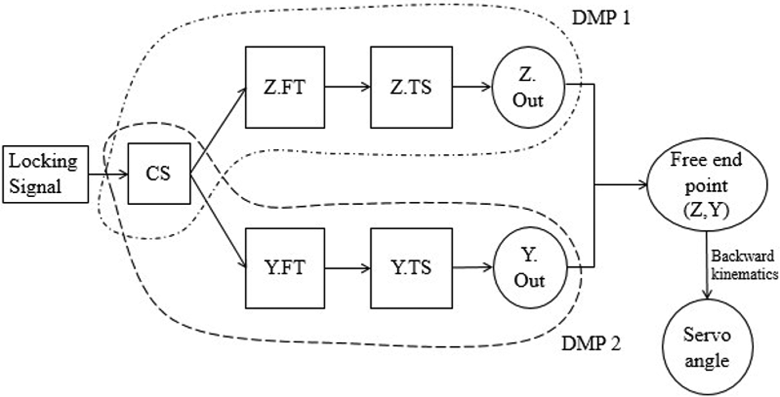
In order to make DMP suitable for quadruped control, we use two DMPs to construct a new elementary module called single leg module (SLM) to control a single leg. Its general structure is shown in Figure 6.

Figure 6.

Structure of an SLM. The output of an SLM is the angle of the servo motor. The point of free end is calculated in Cartesian space. SLM: single leg module.

As we talked above, we use two DMPs to reconstruct a predesign trajectory. But instead of using two separate DMPs, such SLM only uses one canonical system. By doing this, the two DMPs can only keep zero phase lock all the time but reducing the redundancy of this system. The canonical system left can still be used to synchronize with other SLMs. The output of this SLM is the angle of the servo motor, which means we directly control the position of the free end or the foot. In some situation, position control is much easier than force control but makes it impossible to compensate the disturbance in low-level control loop.

Coordination through different SLMs can be different. Like the fundamental topological structures of multiples coupled oscillators, there can be chain type, radial type, ring type and fully connected type. In this work, we use unidirectional radial type (Figure 7).

Figure 7.

Unidirectional radial type used in our work. SLM: single leg module; CC: central controller; UI: user interface.

Central controller is a high level controller which is responsible for external base signal generating and user interface input explanation. So the coordination between four SLMs is achieved by synchronizing them to the same external base signal separately, which generated by the external oscillator which actually shares the same structure as equation (9). The frequency of this external oscillator can be changed directly by changing the value of the τ in it and will not cause any step change of the final output even when τ comes into a negative value, because the four SLMs contain DMP as a natural low-pass filter.

This unidirectional radial type is relatively easy to achieve and control. Since there is no direct connect between any two SLMs, we can assign any SLM’s phase difference without affecting other SLMs and make it easier to predict one SLM’s behaviour.

We choose trot gait here because it’s the most stable one for our quadruped robot in our simulation environment. One thing should be noticed is that real gait relies on lots of things like speed, robot size and so on. Since our control strategy is open loop control actually, the parameters can only be decided by trial and error and obviously a little different from the primary gaits (Table 1).⁶

Table 1.

Primary gaits for quadrupeds.^a

	Front right (p_RF)	Hind left (p_LH)	Hind right (p_RH)
Walk	π	3π/2	π/2
Trot	π	π	0
Pace	π	0	π
Bound	0	π	π

^aPhase increases from 0 to 2π during one period and p_i represents the phase shift with respect to front left leg.

Simulation results and discussion

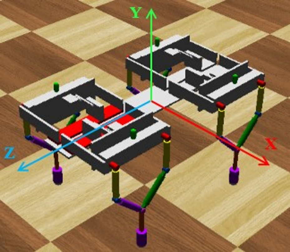
Experiments were done in Webots¹⁸ using a simplified quadruped robot model (Figure 8) on a flat plane. The simulation environment is support by ODE physics engine. Although the robot is simplified, we did some mass adjust considering the real mass allocation, so that this model can be an approximation of the real robot.

Figure 8.

The body coordinate frame Σ_b and the robot horizon in simulation.

Walking in trot gait through open loop control

We chose trot gait as our prime gait, but we did a little modification based on the phase relation in primary gaits. Here in our experiments, we used:

So we subtracted 0.05π from each hind leg’s phase, the difference is shown more clearly in Figure 9. Actually, one can adjust the left side legs’ phase or diagonal legs’ phase instead of the hind legs’. But as we can see in Table 1, we just add π to each hind leg’s phase then we get pace. If we add π/2, then we get walk. Only bound is so much different from the other three gaits, but we can still turn pace into bound through adding π to their diagonal legs’ phase. So the adjustment we made here can be seen as a kind of linear interpolation between walk, trot and pace. One thing can be verified is that different gaits relate to moving speed closely as for one quadruped animal.^19,20 So this kind of adjustment may follow some hidden rules but obviously there still needs a lot of work.

Figure 9.

Modified trot gait used in simulation. Black block represents the stance phase and the white block represents the flight phase.

We measured the height of the centre of robot as the main evaluation of the stability of the robot. The record is showed in Figure 10. The initial height of robot is a little higher, because the mechanical zero point of this parallel structure is at the edge of its work space and we need to move the free end into its work space first. The transition was quite natural without any overshoot. When the robot entered the stable moving state, there was some periodic disturbance. But consider the unit of the data is meter which means the disturbance is within 3 mm. So this result shows the robot entered a good stable state. Figure 11 shows the phase evolution of four legs. The output result was a typical result of a PID controller, which can be verified in equation (15). Although there was no overshoot, the phase lock was quite rapid. The overview of the robot motion is shown in Figure 12.

Figure 10.

Height record of the centre of the robot in moving test. The unit of the height is meter, and the unit of time is second.

Figure 11.

Phase evolution of four legs in moving test. The unit of the vertical axis is π.

Figure 12.

Overview of the robot motion

Speed control

Speed control can be achieved through centre controller shown in Figure 7, which actually changes the frequency of the external oscillator. In simulation environment, we doubled the frequency at 5 s. The height record is shown in Figure 13, phase evolution is shown in Figure 14 and the displacement along forward direction is shown in Figure 15. Although the speed-up technique we used here changes the frequency and holds the phase relation at the same time, it should be noticed that different moving speeds often relate to different phase relation. So there should be some modification of phase relation, as we change the moving speed.

Figure 13.

Height record of the centre of the robot in speed-up test. At 5 s, we double the frequency of the reference oscillator.

Figure 14.

Phase evolution of four legs in speed-up test. The step change of the frequency caused a step change of phase. While due to the injection lock, this disturbance can be eliminated shortly. The unit of the vertical axis is π.

Figure 15.

Record of displacement along forward direction in speed-up test. At 5 s, the moving velocity increased as we double the frequency of the reference oscillator.

Another extreme example of speed controlling is to make the robot move backwards from forwards just by turning the external reference signal into a decreasing slope signal. In other words, we make the τ in external oscillator be its opposite number directly. This kind of tests are not common in quadruped research, while our robot has the symmetry to allow it to move backwards and our controller can also achieve it without any new modifications.

In this test, we turned the oscillator frequency into its opposite value directly at 5 s. The height record is shown in Figure 16, phase evolution is shown in Figure 17, displacement record is shown in Figure 18 and canonical system output of fore left leg is shown in Figure 19. The disturbance in Figure 17 was different from Figure 14, since here we decreased the external oscillator frequency instead of increasing it.

Figure 16.

Height record of robot in backward moving test. At 5 s, we set the frequency into its negative value directly. The disturbance of the height becomes stronger while still keeps in a limited range.

Figure 17.

Phase evolution of four legs in backward moving test. At 5 s, we set the frequency to be its negative value. The unit of the vertical axis is π.

Figure 18.

Displacement record of robot’s forward direction in backward moving test. When we set the frequency to be its negative value at 5 s, the robot turned into moving backward rapidly without any stops.

Figure 19.

Canonical system output of fore left leg in backward moving test. The solid line represents the canonical system output of fore leg’s SLM. The dashed line represents the output of the external oscillator. SLM: single leg module.

The transition progress is shown more clearly in Figure 19, from where we can see that the injection lock keeps both of the frequency and phase stay the same.

Turning control

Turning control is achieved by using the same techniques with controlling a differential wheel robot. Reminding that we decomposed the trajectory into two directions in SLM, here we just need to modify the z direction amplitude of one side legs. So that we can make the average speed of two sides different, then the robot can turn without any effects on phase relations.

In our tests, we made the z direction amplitude of right side half to make the robot turn right from 5 s to 10 s. The height record and phase evolution of the robot are nothing different from the moving test, so we don’t show them here. Figure 20 shows the robot moving trajectory projected on the walking plane, from which we can see the effect of this turning technique more clearly. It should be noticed that the turning is finished in several periods discretely, as the quadruped moves in periodic and discretely motion.

Figure 20.

Two-dimensional trajectory recorded in turning test. This trajectory is the projection of robot three-dimensional trajectory on the walking plane in Σ_g. Dotted line indicates the robot was doing a turning motion.

Interesting phenomena of open loop control

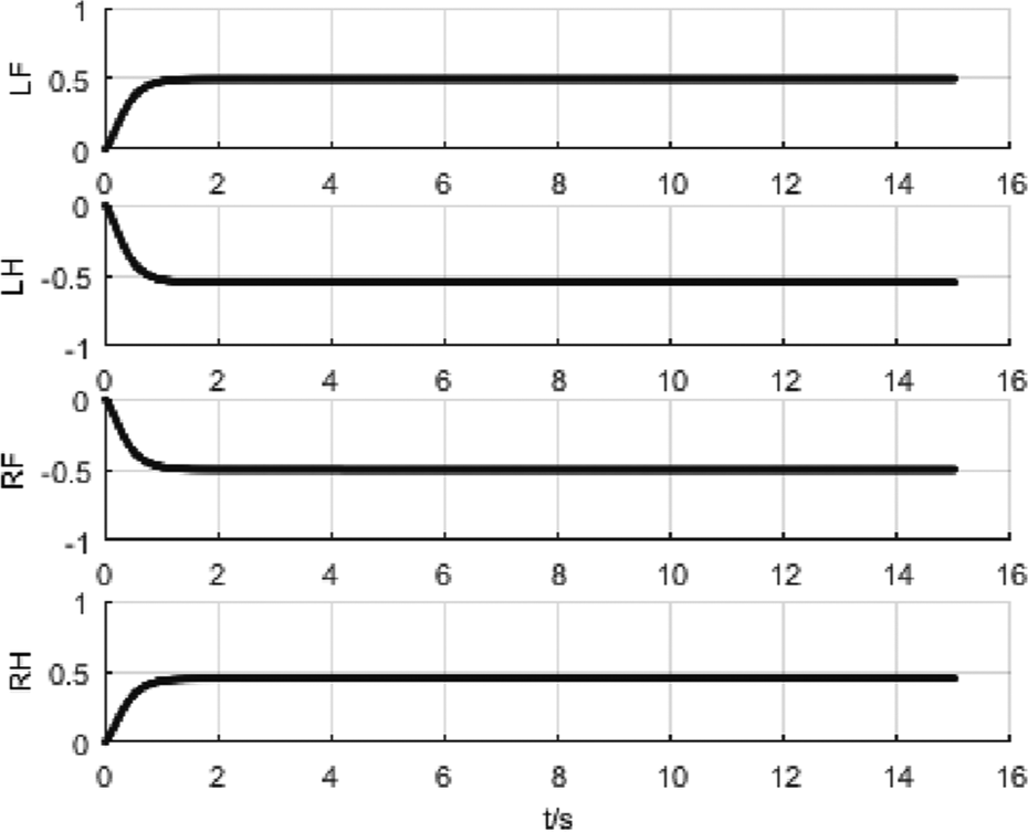
Although the open loop control exists many drawbacks, it is the basis of a closed loop control. In our simulation tests, we add a touch sensor at the end of each leg, from which we can know if the leg touch the ground. The record data in moving test is plotted in Figure 21.

Figure 21.

Y direction output of fore left leg’s SLM. The dotted lines indicate the leg touches the ground while the solid lines indicate the leg leaves the ground. SLM: single leg module.

Actually, we have already assigned the stance and flight period just when we designed the predesign trajectory in Figure 4. Obviously, we want the leg touch the ground when it moves on the straight line and leaves the ground when it comes to the arc. But in our simulation results as showed in Figure 21, the fore left cannot leave or touch the ground in time. Honestly, we cannot guarantee the robot stability even when the simulation record meets the design, and it shouldn’t be that strange if the two don’t meet because we use open loop control here.

Conclusion

In this article, we proposed a modular quadruped robot and an online gait generator for the control of walking. The robot is constructed by four independent leg modules. Each leg module includes a five-bar mechanism as its main structure. This five-bar mechanism makes the two leg servos directly attached to the robot trunk, thus reduce the leg mass and balance the payload of two servos. A method of calculating forward and backward kinematics of this five-bar mechanism is also present. This method does not include many trigonometric functions and solve both the forward and backward kinematics based on a simple three-point question.

The controller in the article can learn a given trajectory and regenerate it real time. Moreover, this controller is able to adjust the output frequency and two independent degrees’ amplitude. Due to the DMP’s natural coordination ability and unidirectional radial coordination type we used, we can control the robot to move in a certain trot gait on a flat plane The output of the controller is explained in Cartesian space, which makes it suitable for different kinds of leg design and easy to change the shape of output trajectory.

Although our controller is an open loop one, the robot is able to speed-up or even move backwards without any stop. Turning is achieved by taking the same techniques used in differential wheels robot. All the tests about the above tasks are finished in Webots simulation environment, showing that it’s a simple but effective way to control a quadruped robot.²¹

Loss of sensors feedback makes our controller cannot walk on uneven ground stably. More research will be done about how to adjust the phase relation and ratio of stance and flight phase. Since the controller is not complicated and very open so far, we believe the introduction of feedback will not cause a big modification of this controller’s structure.

Footnotes

Acknowledgements

This article is a revised and expanded version of a paper entitled Control of quadruped walking robots using motor primitives presented at the 18th International Conference on Climbing and Walking Robots (CLAWAR’15), Hangzhou, China, September 6–9, 2015.²¹

Declaration of conflicting interests

The author(s) declared no potential conflicts of interest with respect to the research, authorship, and/or publication of this article.

Funding

The author(s) disclosed receipt of the following financial support for the research, authorship, and/or publication of this article: The financial supports by National Natural Science Foundation of China (51305396 & U1509210) and the Fundamental Research Funds for the Central Universities (2-2050205-16-061) are acknowledged.

References

Bruzzone

Quaglia

. Review article: locomotion systems for ground mobile robots in unstructured environments. Mech Sci 2012; 3(2): 49–62.

Kolter

Rodgers

. A Control architecture for quadruped locomotion over rough terrain. In: Robotics and Automation, ICRA 2008. IEEE International Conference, 19–23 May 2008, pp. 811–818. IEEE, Pasadena, CA: IEEE.

Estremera

de Santos

. Generating continuous free crab gaits for quadruped robots on irregular terrain. IEEE Trans Robo 2005; 21(6): 1067–1076.

Estremera

Gonzalez De Santos

. Free gaits for quadruped robots over irregular terrain. Int J Robot Res 2002; 21(2): 115–130.

Ijspeert

. Central pattern generators for locomotion control in animals and robots: a review. Neural Netw 2008; 21(4): 642–653.

Tran

Koo

Lee

. Central pattern generator based reflexive control of quadruped walking robots using a recurrent neural network. Rob Auton Syst 2014; 62(10): 1497–1516.

Kimura

Fukuoka

Cohen

. Biologically inspired adaptive walking of a quadruped robot. Philos Trans R Soc A Math Phys Eng Sci 2007; 365(1850): 153–170.

Kimura

Fukuoka

CoChen

. Adaptive dynamic walking of a quadruped robot on natural ground based on biological concepts. The International Journal of Robotics Research 2007; 26(5): 475–490.

Righetti

Ijspeert

. Pattern generators with sensory feedback for the control of quadruped locomotion. In: Robotics and Automation, 2008. ICRA 2008. IEEE International Conference, 19–23 May 2008. Pasadena, CA: IEEE.

10.

Zhou

Low

. Design and locomotion control of a biomimetic underwater vehicle with fin propulsion. IEEE/ASME Trans Mechatronics 2012; 17(1): 25–35.

11.

Ijspeert

Crespi

Ryczko

. From swimming to walking with a salamander robot driven by a spinal cord model. Science 2007; 315(5817): 1416–1420.

12.

Sprowitz

Tuleu

Vespignani

. Towards dynamic trot gait locomotion: design, control, and rxperiments with cheetah-cub, a compliant quadruped robot. Int J Robot Res 2013; 32(8): 932–950.

13.

Ijspeert

Nakanishi

Schaal

. Learning rhythmic movements by demonstration using nonlinear oscillators. In: Intelligent Robots and Systems, 2002. IEEE/RSJ International Conference, September 30–October 4 2002, pp. 958–963. Lausanne, Switzerland: IEEE.

14.

Ijspeert

Nakanishi

Hoffmann

Pastor

Schaal

. Dynamical movement primitives: learning attractor models for motor behaviors. Neural Comput 2013; 25(2): 328–373.

15.

Schaal

Mohajerian

Ijspeert

. Dynamics systems vs. optimal control - a unifying view. In: Cisek

Drew

Kalaska

, eds. Progress in Brain Research. Oxford: Elsevier; 2007, pp. 425–445.

16.

Degallier

Ijspeert

. Modeling discrete and rhythmic movements through motor primitives: a review. Biol Cybern 2010; 103(4): 319–338.

17.

Pikovsky

Rosenblum

Kurth

. Synchronization: a universal concept in nonlinear sciences. Cambridge: Cambridge University Press, 2003.

18.

Michel

. Webots: professional mobile robot simulation. Int JAdv Robot Syst 2004; 1(1): 39–42.

19.

Hildebrand

. Symmetrical gaits of horses. Science 1965; 150(3697): 701–708.

20.

Hildebrand

. Analysis of asymmetrical gaits. J Mammal 1977; 58(2): 131–156.

21.

Zhou

Wang

. Control of quadruped walking robots using motor primitives. In The 18th International Conference on Climbing and Walking Robots CLAWAR’15, 6–9 September 2015, Hangzhou, China.

An online gait generator for quadruped walking using motor primitives

Abstract

Keywords

Introduction

Design of the quadruped robot

Design of the leg module

Kinematics of the five-bar mechanism

Dynamical movement primitives

Basic structure of DMP

Amplitude and frequency scale

Coordination between different DMPs

Proposed controller

Predesign trajectory

Single leg module and the overall controller

Simulation results and discussion

Walking in trot gait through open loop control

Speed control

Turning control

Interesting phenomena of open loop control

Conclusion

Footnotes

Acknowledgements

Declaration of conflicting interests

Funding

References