Sage Journals: Discover world-class research

Abstract

Robots that operate in static environments with fixed obstacles are crucial for automating processes in industries such as manufacturing, warehousing, and healthcare. Although these environments are static, designing a navigation algorithm that achieves high accuracy, reasonable efficiency, and low computational complexity remains a significant challenge. Besides performing well in familiar settings, the algorithm must also be capable of generalizing to other static environments with different obstacle configurations.To address these challenges, this paper presents a navigation algorithm based on deep reinforcement learning (DRL), specifically a combination of double Q-networks, multi-stage learning, and priority experience replay (PER). This algorithm is referred to as PER-MS-DDQN. The key innovation of this research is the simultaneous development of a new reward function derived from the A* algorithm and a new definition of robot states. This combination enhances navigation accuracy, speeds up the learning process, and mitigates the issue of scattered rewards. The proposed algorithm was initially trained in a basic static environment using Grid World and subsequently evaluated both in this familiar setting and in larger, more complex static environments, including the ROS2 software environment. Additionally, the algorithm was tested in a real-world environment. The results indicate that over 500 episodes, the robot achieved a success rate of 99% in reaching its goals. Moreover, there was a significant improvement in both accuracy and navigation time compared to previous methods. These findings demonstrate the practicality and efficiency of the proposed algorithm and its ability to generalize in real-world scenarios.

Keywords

Navigation mobile robot reinforcement learning MS_PER_DDQN unknown environments

Introduction

The navigation of mobile robots in static environments with fixed obstacles presents a fundamental challenge in robotics as well as in the automation of industrial processes, warehousing, and healthcare. Although these environments are largely static, creating an algorithm that operates with high accuracy, low computational complexity, and robust generalization capabilities remains a significant challenge. In recent years, the application of artificial intelligence methods, particularly machine learning and deep reinforcement learning, has significantly enhanced robots’ abilities to make independent and adaptive decisions in their environments. Navigation processes have been simplified through the exploration of end-to-end approaches.¹ To improve adaptability, Q-learning has been applied to adjust the parameters within the dynamic window algorithm.² Koraim et al. developed a robust controller based on artificial intelligence to enhance the performance of mechanical arms.³

Advancements in self-learning frameworks have been achieved by combining imitation learning with deterministic policy gradients.⁴ Model convergence has been accelerated through the integration of dual learning algorithms,⁵ while decision-making accuracy in crowded settings was improved by merging differential and imitation learning approaches.⁶ Furthermore, the stability of reinforcement learning within mapless navigation has been enhanced through the design of proximal policy networks.⁷ Despite their different objectives, these various efforts collectively contribute to the advancement of navigation capabilities for mobile robots.⁸

Reinforcement learning is a machine learning method where an agent makes optimal decisions by interacting with its environment and receiving rewards. The Q-learning algorithm enables the agent to acquire necessary knowledge through experience and trial and error, without relying on labeled data or prior knowledge of the environment.⁹ For example, local navigation systems have been developed by integrating deep reinforcement learning with satellite positioning.¹⁰ To enhance performance on curved paths, a controller based on a double deep Q-network was created.¹¹ Furthermore, a method based on the proximal policy algorithm has been introduced, which emphasizes population navigation in dynamic environments.¹² Additionally, a hybrid framework that combines reinforcement learning and hazard awareness was designed to safely guide robots in complex and unknown environments.¹³ To improve decision-making structures in reinforcement learning, various studies have been conducted with different objectives, ultimately aiming to enhance algorithm performance. For example, Wang et al. proposed a dual structure architecture for neural networks to better evaluate the action selection policy in model-free reinforcement learning.¹⁴ Similarly, a deep learning-based protocol has been developed to increase the stability of routing in dynamic networks, which successfully improves both the convergence rate and routing accuracy using a double deep Q-network.¹⁵

To enhance the performance of reinforcement learning in robot navigation, several studies have focused on the multi-stage prioritization of experiences, resulting in advanced methodologies. Peng et al. combined multi-stage updating with a two-depth Q-network and various reward systems, which significantly improved the accuracy and success rate of mobile robot navigation in experiments using laser sensors.¹⁶ In dynamic environments, a hybrid approach combining supervised and reinforcement learning has been employed to guide autonomous vehicles, demonstrating effective decision-making in both simulated and real-world scenarios.¹⁷ Training efficiency and stability have been further optimized through specialized frameworks and architectures. Methods aimed at enhancing convergence and reducing training time have utilized experience prioritization and large datasets, replacing traditional priority-based methods with balanced experience replay to improve overall model performance and stability.^18,19 Furthermore, improved versions of deep two-Q-networks featuring dual architectures and prioritized experience replay have been shown to outperform traditional algorithms in complex environments such as mazes.²⁰ To increase learning stability and accuracy, algorithms based on double-deep Q-networks have also incorporated second-order time difference and tree structure techniques, effectively reducing convergence time and stabilizing the reward function.²¹

In ongoing research focused on enhancing reinforcement learning, several studies have introduced effective approaches that emphasize the multi-stage structures of the Q-algorithm. To improve the accuracy of Q-value estimation and manage the behavior of high-speed vehicles in complex environments, multi-stage double and dual Q-network structures have been developed. These methods replace traditional single-stage rewards with multi-stage rewards and incorporate experience classification, resulting in more stable and effective decision-making.^22,23 Further advancements include the development of a “multi-stage deep Q-network with priority” algorithm. This innovation reduces the number of training episodes required and allows for effective learning using only visual inputs and game scores, achieving performance levels comparable to those of professional human players.²⁴ Additionally, navigation tasks have been simplified by breaking down paths into sub-goals using a multi-stage double deep Q-network structure.²⁵ This approach reduces decision-making complexity, leading to more precise robot guidance, fewer collisions with obstacles, and lowered computational costs.

Recent research has increasingly focused on enhancing the navigation capabilities of mobile robots by optimizing reward function structures and improving sensor data processing. For example, the development of azimuth and partial reward functions has been shown to enhance guidance accuracy, significantly reducing aimless exploration and accelerating the learning process of the agent.²⁶ Precise, real-time navigation in complex environments has been achieved through the integration of advanced algorithms with LiDAR sensors, specifically implemented on the ROS2 platform.²⁷ Moreover, decision-making has been further optimized through deep Q-network-based systems that facilitate intelligent routing in challenging environments.²⁸ To navigate unfamiliar areas without requiring an initial map, multi-segment systems have been designed to effectively combine sensor data with reinforcement learning, enabling autonomous movement.²⁹ Finally, transforming LiDAR data into network maps has been employed to support effective training and reliable obstacle avoidance using the deep Q-algorithm.³⁰

Open-source tools like ROS and the Gazebo simulator provide an effective platform for developing and evaluating reinforcement learning algorithms for mobile navigation. Within this framework, a novel real-time navigation algorithm for mobile robots has been introduced using federated reinforcement learning. This approach, implemented specifically with ROS and Gazebo, employs original models to improve navigation performance and enhance generalizability across unfamiliar environments.³¹ Additionally, deterministic policy correction algorithms have been applied within the ROS2 environment to optimize autonomous navigation in continuous action spaces. Simulation results in Gazebo have demonstrated the effectiveness of navigating paths in unknown environments, even when facing various damage factors.³²

The proposed algorithm enables accurate autonomous navigation in unknown static environments without requiring a predefined map. This is achieved through a novel state structure—based on the robot's relative position and environmental features—and a goal-oriented reward function aligned with the A* algorithm. Together, they reduce decision-making ambiguity, prevent aimless exploration, and enhance learning stability. Discretely modeled test environments allow precise control over structural complexity, though the multi-stage design and discretization introduce computational challenges, which are addressed in the analysis section. In this work, a framework called PER-MS-DDQN is proposed for mobile robot navigation, in which DDQN, PER, and MS algorithms are integrated. To effectively guide the robot toward the target point and reduce training time, the reward function A* is utilized. Furthermore, to enhance the agent's performance, a new state is defined for the robot, initialized using a trial-and-error approach. Section 2 discusses the performance improvements of the reward function and the design of the mobile robot navigation model. Section 3 provides a comprehensive introduction to the model's training and learning parameters. Finally, the effectiveness of the proposed methods is evaluated and verified through simulations and experimental tests.

Theoretical foundations and associated algorithms

Reinforcement learning

Reinforcement learning is a powerful branch of machine learning that effectively directs an agent's behavior in dynamic environments using a Markov decision process (MDP). In this robust framework, the agent observes the current state of the environment ( $s_{t}$ ) and decisively selects an action ( $a_{t}$ ) from a set of viable options ( $A (s_{t})$ ). After executing the chosen action, the environment transitions to a new state ( $s_{t + 1}$ ), and the agent is rewarded with ( $r_{t + 1}$ ). This dynamic cycle of interaction continues until the final step (T). The primary objective of the agent is clear: to maximize the total rewards accumulated over the course of the episode. The sum of these rewards is calculated using the following equation:

G_{t} = \sum_{t^{'} = t}^{T} γ^{t^{'} - t} R_{t^{'} + 1}

(1)

In Equation (1), the discount factor, represented by $γ$ , ranges from 0 to 1. For optimal function calculations, classical boosting algorithms are effectively formulated using mathematical frameworks such as Bellman's optimality equations. Equation (2) clearly defines how to update the value of Q by leveraging the principles of current value and the maximum potential future value.

q (s_{t}, a_{t}) = E [r_{t + 1} + γ m a x_{a_{t + 1}} q_{π} (s_{t + 1}, a_{t + 1})]

(2)

To gradually learn these values, Equation (3) is utilized for the subsequent update:

q_{π} (s_{t}, a_{t}) \leftarrow q_{π} (s_{t}, a_{t}) + α [r_{t + 1} + γ m a x_{a} q_{π} (s_{t + 1}, a_{t}) - q_{π} (s_{t}, a_{t})]

(3)

The variable (α) clearly signifies the learning rate. These equations empower the agent to update Q values optimally, significantly enhancing its decision-making policy through thorough empirical analysis of interactions.

DQN and DDQN algorithms

In complex environments, the deep Q network (DQN) algorithm utilizes neural networks to estimate the values of the Q function for state–action pairs. The target value of Q is calculated according to Equation (4):

q (s_{t}, a_{t}; θ) = r_{t + 1} + γ q (s_{t + 1}, m a x_{a_{t}} q_{π} (s_{t + 1}, a_{t}, θ); θ^{'})

(4)

To minimize overestimation, the DDQN algorithm employs two independent networks. The target value in DDQN is defined by Equation (5):

Y_{t}^{Q} = r_{t + 1} + γ q (s_{t + 1}, m a x_{a} q_{π} (s_{t + 1}, a_{t}, θ); θ)

(5)

The value of double Q is derived from Equation (6):

Y_{t}^{d o u b l e} (s_{t}, a_{t}; θ^{'}) \equiv r_{t + 1} + γ q (s_{t + 1}, m a x_{a} q_{π} (s_{t + 1}, a_{t}, θ); θ^{'})

(6)

Priority experience reply memory

Priority experience replay (PER) enhances learning efficiency by prioritizing experiences with higher informational value, even if they occur less frequently. Its implementation faces two key challenges: automatic priority assignment and efficient sampling. To address these, rank-based and proportional sampling methods are used, balancing randomness with targeted selection. In proportional sampling, the likelihood of selecting an experience is proportional to its temporal difference (TD) error, encouraging the agent to focus on more informative transitions. The replay memory stores experiences in the format (s_t, a_t, r_t, s_t+1, done, p_t), where the priority p_t is determined by the transition's TD error δ_i. Following Equation (7), this prioritization allows the agent to focus on transitions that offer the highest learning potential.

δ_{i} = r_{t} + γ Q_{θ^{'}} (s_{t + 1}, a r g m a x_{a} q (s_{t + 1}, a) : θ^{'}) - q (s_{t}, a_{t} : θ)

(7)

Proposed algorithm

To improve the PER-DDQN algorithm's performance, multi-step learning was integrated to stabilize training and reduce fluctuations. With the addition of a goal-oriented reward function and modified inputs, the enhanced algorithm showed superior results in Section 3.3. Key metrics—including reduced episode time, higher cumulative rewards, closer Q-value alignment, and increased success rate—demonstrate improvements in speed, stability, and learning efficiency compared to the basic DDQN. Equation (8) illustrates how to update the value of the function Q according to the proposed algorithm, and it explains how to update the value of the function q based on the same algorithm.

\begin{aligned} q (s_{t}, a_{t}; θ) = \sum_{i = 0}^{i = n - 1} γ^{i} r_{t + i} \\ + γ^{n} q (s_{t + 1}, a r g m a x Q (s_{t + n}, a r g m a x Q (s_{t + n}, a, θ), θ); θ^{'}) \end{aligned}

(8)

Designing an enhanced viewing environment for robot navigation

In this paper, as it shown in Figure 1 the accuracy of robot guidance in complex environments is improved by redesigning the observation space of the learning network. The network inputs are defined to include the robot's current position, represented by normalized values for norm-robot-x and norm-robot-y. Additionally, sub-goals are incorporated, which are determined using the A* algorithm and consist of norm-goal-x and norm-goal-y values. o enhance the agent's understanding of its surroundings, the robot's distance from obstacles in four main directions is assessed, and these distances are categorized into five levels ranging from “very far” to “dangerous”.

Figure 1.

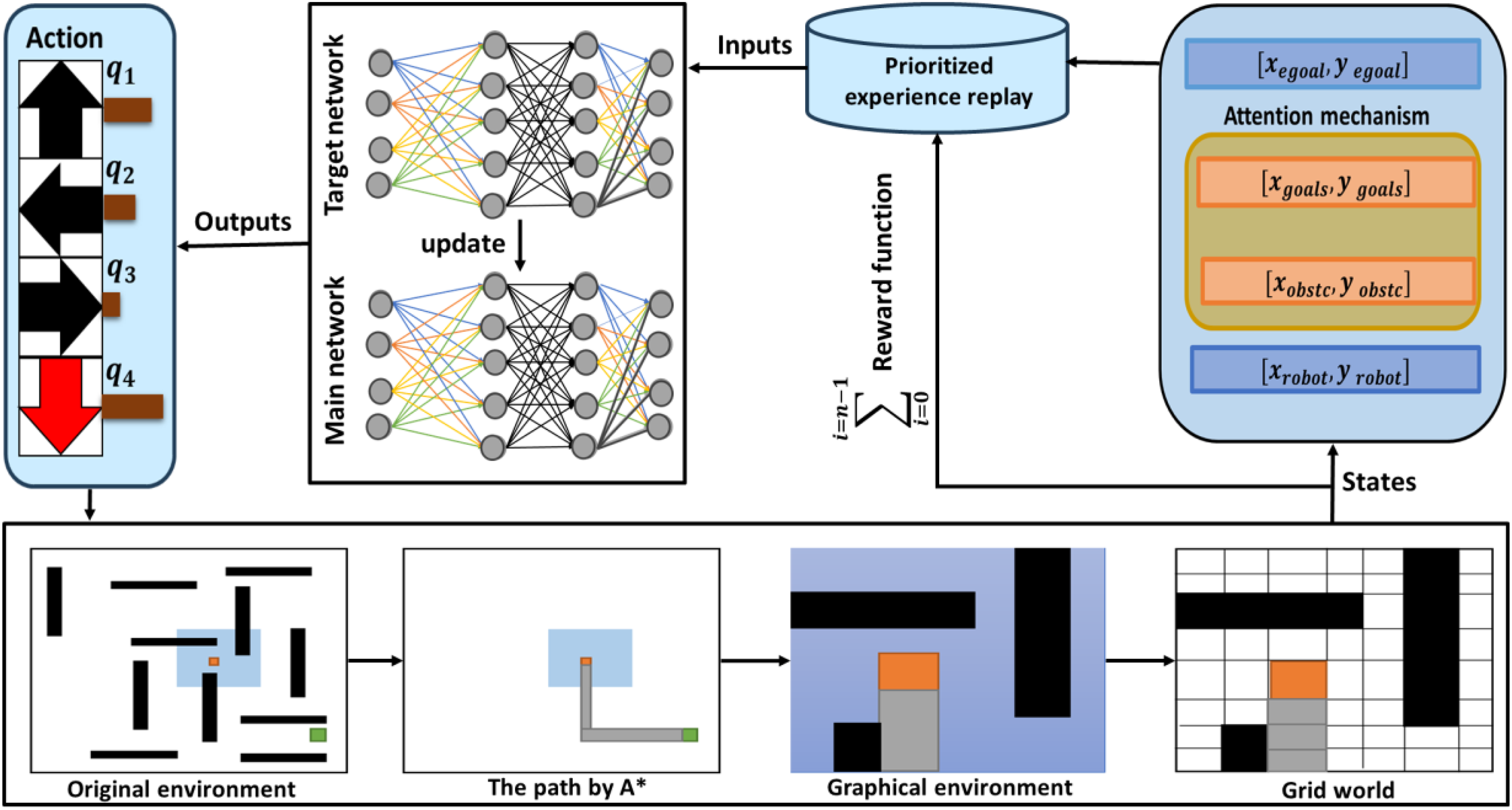
Schematic diagram of the MS-PER-DDQN algorithm.

In this system, Level 1 (one block) is designated as the “dangerous” zone because the physical footprint of the TurtleBot3 Burger occupies a significant portion of a single cell, making any obstacle in the immediate or adjacent block a collision risk. Level 2 (two blocks) represents the “close” zone where the agent must initiate evasive maneuvers, while Levels 3 and 4 serve as “medium” and “far” buffers, respectively. Finally, Level 5 (five blocks) is categorized as “very far,” representing the maximum possible distance within the grid boundaries.

To address the challenges of navigation in complex environments, several strategies are adopted: precise and descriptive definitions of obstacle positions are provided, negative rewards are applied for obstacle encounters or inefficient paths, observations are prioritized to emphasize essential information, and the distance from obstacles is given precedence over the target position when proximity to obstacles is high.

Proposed reward function

In this method, the robot receives continuous feedback in complex environments by introducing appropriate inputs. This feedback accelerates the navigation learning process through a specifically designed dense reward function. This function dynamically adjusts the importance of examples and minimizes the need for predetermined sub-goals. It assigns positive rewards for reaching a final goal or sub-goals and negative rewards for collisions or unnecessary movements, utilizing attention mechanisms. The reward function is conditionally defined in Equation (9).

r (t) = {\begin{matrix} r_{1} < 0 & i f c_{r o b t} = c_{f r e e} \\ \begin{matrix} r_{2} < 0 \\ \begin{matrix} r_{3} > 0 \\ r_{4} > 0 \end{matrix} \end{matrix} & \begin{matrix} i f c_{r o b t} = c_{o b s t e c l e} \\ \begin{matrix} i f c_{r o b t} = c_{e n d g o a l} \\ i f c_{r o b t} = c_{g o a l s} \end{matrix} \end{matrix} \end{matrix}}

(9)

Where $c_{g o a l s}$ represents the reward for reaching intermediate sub-goals, $c_{e n d g o a l}$ is the reward for reaching the final target, and $c_{o b s t e c l e}$ denotes the penalty for collisions. Additionally, $c_{r o b t}$ and $c_{f r e e}$ represent the robot's state and the free space, respectively.

The A* algorithm determines the locations of sub-goals based solely on the robot's current position and the final locations of the goals, without taking obstacles into account. As a result, the path that the robot follows to reach the goals remains fixed and is provided to the robot only once.

Training and testing

Network training process

The agent was trained episodically in a 2D environment, where each episode ended upon reaching the goal, colliding with an obstacle, or exceeding 128 steps. The training environment was a 2 × 2 m area featuring two phases: a basic phase (obstacle-free) and an advanced phase (up to three static obstacles). Inputs—including positions, directional distances, and A* subgoals—were normalized and fed into an MLP with RELU and HC Linear activations. Training was accelerated using TensorFlow and GPU. The agent followed an epsilon-grid policy, with epsilon decreasing linearly from 0.9 to 0.09 during training and fixed at 0.5 during testing.

As detailed in Table 1, the architecture consists of three dense layers (1024, 4048, and four neurons) totaling 417,660 trainable parameters. Experiences were stored in a prioritized replay buffer (capacity: 1024) and selected based on TD error. Multi-stage regression was used to compute target Q-values, and the main network was updated via backpropagation with delayed synchronization. Training was performed over 3300 steps with a batch size of 64, gamma set to 0.99, and hyperparameters: Learning rate = 0.3, alpha = 0.5, beta = 0.3, tau = 0.6.

Table 1.

Trained network.

Layer (type)	Output shape	Param
Dense	(None, 1024)	11264
Dense	(None, 4048)	4149200
Dense	(None, 4)	16196

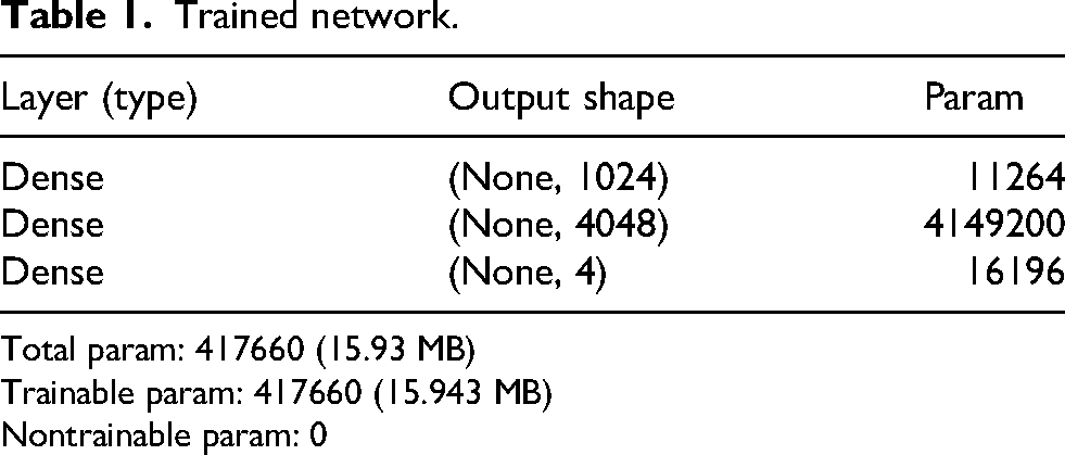
Total param: 417660 (15.93 MB)

Trainable param: 417660 (15.943 MB)

Nontrainable param: 0

The robot's proximity to obstacles was classified into three levels: “far,” “close,” and “direct collision.” Training duration ranged from 3 to 24 h on a desktop computer. During training, the agent interacted directly with the simulated environment, using lidar observations and positional data to select actions, receive rewards, and update its neural network parameters. In the evaluation phase, the trained network was deployed without further updates, enabling the agent to navigate based solely on the learned policy.

Grid world

To showcase the effectiveness of the trained agent in a static network-based environment, a series of simulated environments represented as grid maps was designed and tested. Each test scenario was derived from a core configuration, with structural variations introduced by modifying the underlying network. Static obstacles were positioned in various grid cells, arranged either in a scattered layout or in a maze-like configuration between the starting and goal points.

Mobile robot network and navigation training

As shown in Figure 2(a), the MS-PER DDQN algorithm achieves faster convergence, reaching a reward above 300 after 3300 episodes and a higher final average reward compared to other methods. The proposed approach also exhibits lower reward fluctuations, demonstrating improved stability and learning efficiency in comparison to the standard DDQN. In Figure 5(b), the MS-PER-DDQN algorithm maintained a more stable episode duration throughout the training process, resulting in more effective learning and improved performance stability. It should be noted that the episode duration shown in the chart solely reflects the agent's interaction time within the environment. The actual training time, however, involves additional computational processes such as neural network evaluations, weight updates, prioritized experience sampling, and data logging, which collectively result in a significantly longer overall training duration.

Figure 2.

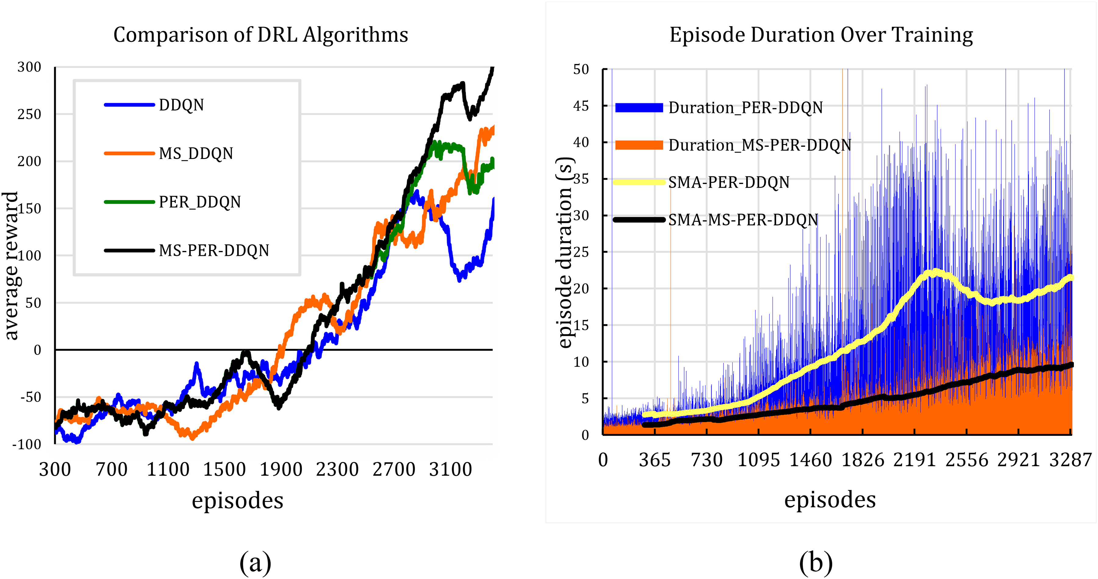
(a) Training reward comparison, (b) episode duration comparison.

In Figure 3, it is evident that the MS-PER DDQN algorithm surpasses other methods in both the “final 500 episodes” (with an average reward of 300.8) and the “entire simulation process” scenarios (with an average reward of 44.1).This advantage, when compared to the baseline double deep Q-network (DDQN), has led to significant improvements in both cases. The primary reason for this difference is the combination of the prioritization of experience replay (PER) mechanism and multi-stage updates. These enhancements accelerate learning and minimize the bias associated with delayed rewards.

Figure 3.

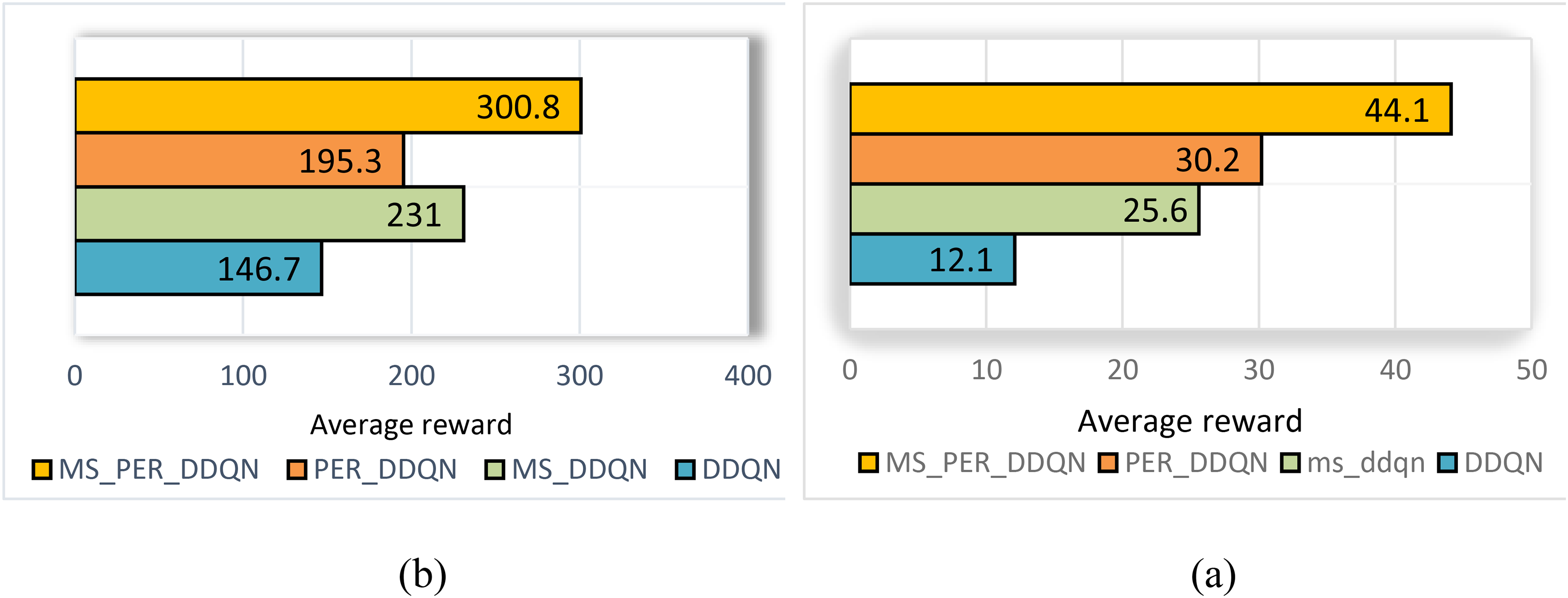
Comparison of average rewards obtained: (a) in the last five hundred episodes and (b) throughout the entire simulation process.

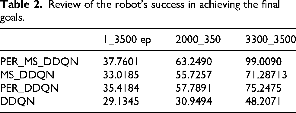
As detailed in Table 2, in the early stages, the combination of PER_MS_DDQN achieves a success rate of approximately 38%. These early failures are primarily due to random collisions as the agent explores the grid map and learns to interpret Lidar signals. This rate increases to about 63% in the intermediate stage; at this point, the agent still faces challenges similar to the early stage, but it demonstrates a more refined data processing capability and a more stabilized policy, allowing it to navigate more effectively while still refining its path through complex areas. In the final stage, the success rate nearly reaches 99%. In comparison, the other methods, including MS_DDQN, PER_DDQN, and DDQN, achieve lower final stage success rates because they lack the combined efficiency of prioritized sampling and multi-step lookahead needed to navigate complex static configurations.

Table 2.

Review of the robot's success in achieving the final goals.

	1_3500 ep	2000_350	3300_3500
PER_MS_DDQN	37.7601	63.2490	99.0090
MS_DDQN	33.0185	55.7257	71.28713
PER_DDQN	35.4184	57.7891	75.2475
DDQN	29.1345	30.9494	48.2071

To evaluate the stability of the algorithms numerically, the standard deviation of the rewards was examined across two different scenarios. As shown in Figure 4, the standard deviation changes are illustrated in 100-episode intervals, demonstrating a reduction in fluctuations and a gradual convergence of the MS-PER-DDQN algorithm in comparison to both DDQN and MS-DDQN.

Figure 4.

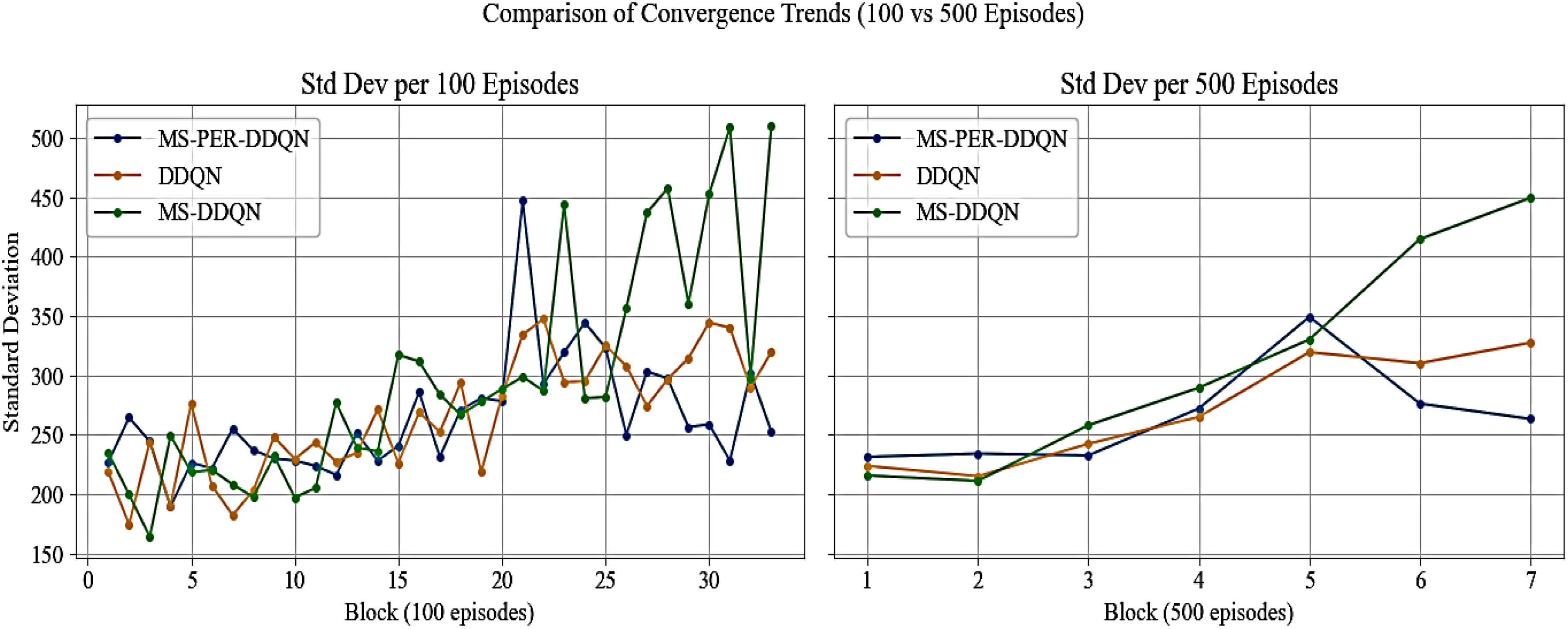
Variations in the standard deviation of algorithm rewards.

Additionally, the same analysis was conducted using 500-episode intervals, providing a more detailed view of the stable trends observed in MS-PER-DDQN. This numerical comparison validates the effectiveness of combining multi-step and prioritized experience replay (PER) in enhancing the stability and performance of the agent in complex environments.

Figure 5 illustrates the PER-MS-DDQN algorithm's learning dynamics by comparing Q1 (actual network output) and Q2 (target value). Over training episodes, the gap between Q1 and Q2 narrows, indicating strong convergence and stable learning. The upward trend of SMA_Q1 and SMA_Q2 curves reflects improved agent performance, as higher Q-values suggest better rewards and more effective decision-making in complex environments.

Figure 5.

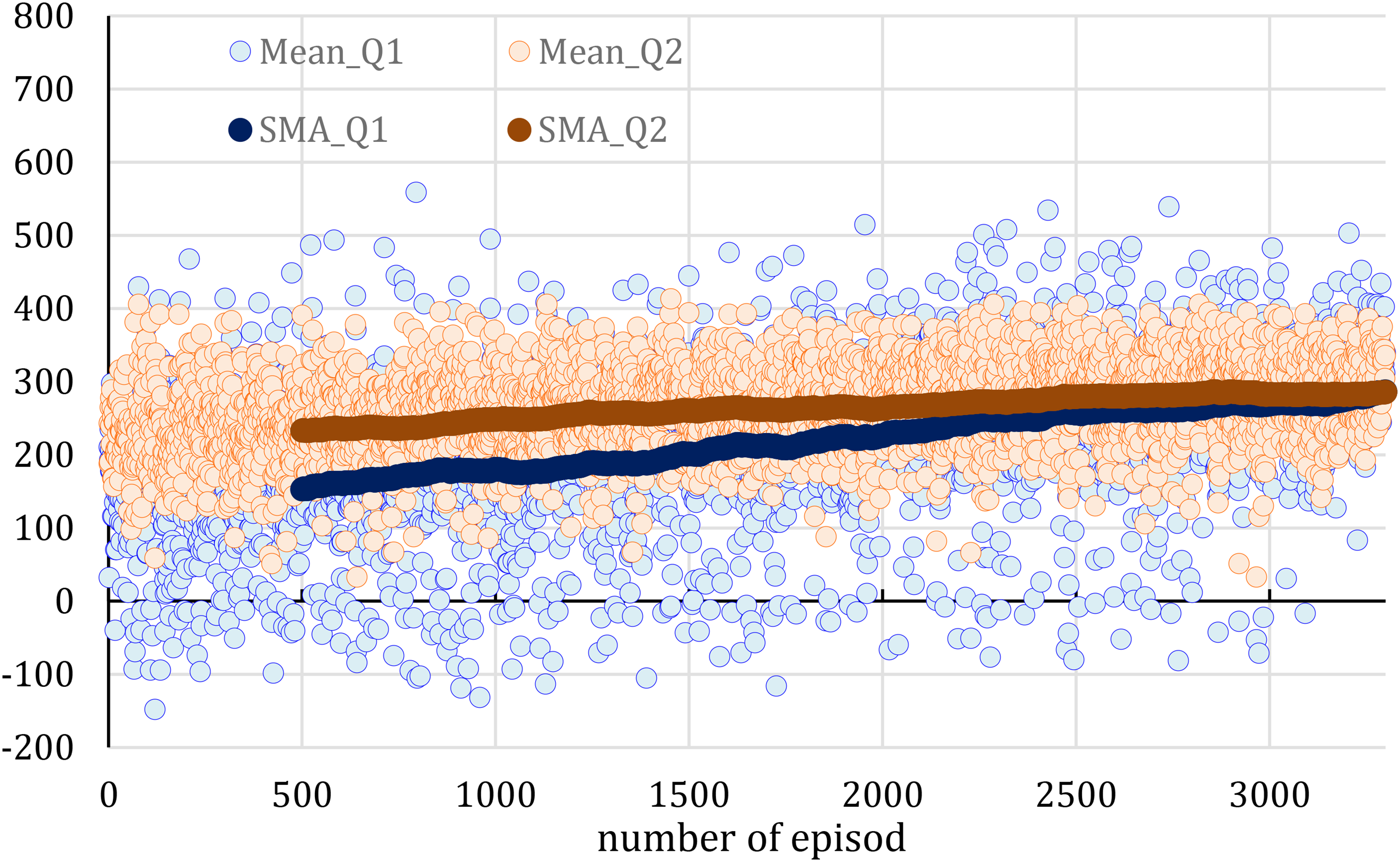
Evaluating learning stability through the convergence of Q1 and Q-Target.

Testing in grid worlds

To demonstrate the effectiveness of the trained agent in a static network-based environment, a series of simulated environments in the form of grid maps were designed and tested. Each experimental environment is based on a core scenario, from which various modifications are made to the network structure to create different scenarios. These environments include static obstacles placed in various cells, arranged either randomly or in a maze-like configuration between the starting point (R) and the goal point (G). Free cells are represented in purple, while cells containing obstacles are marked in blue. This color-coding helps to visually and structurally distinguish between the components of the environment and the traversable paths.

Test 1

This section evaluates the performance of the trained agent in a 10 × 10 environment containing 16 static obstacles. In this scenario, as shown in Figure 6, the initially proposed path passed through an area with two static obstacles. When the agent entered the visibility range of these obstacles, it adjusted its path by taking a controlled detour. This change necessitated the discovery of a shorter geometric path due to the specific positioning of the obstacles.

Figure 6.

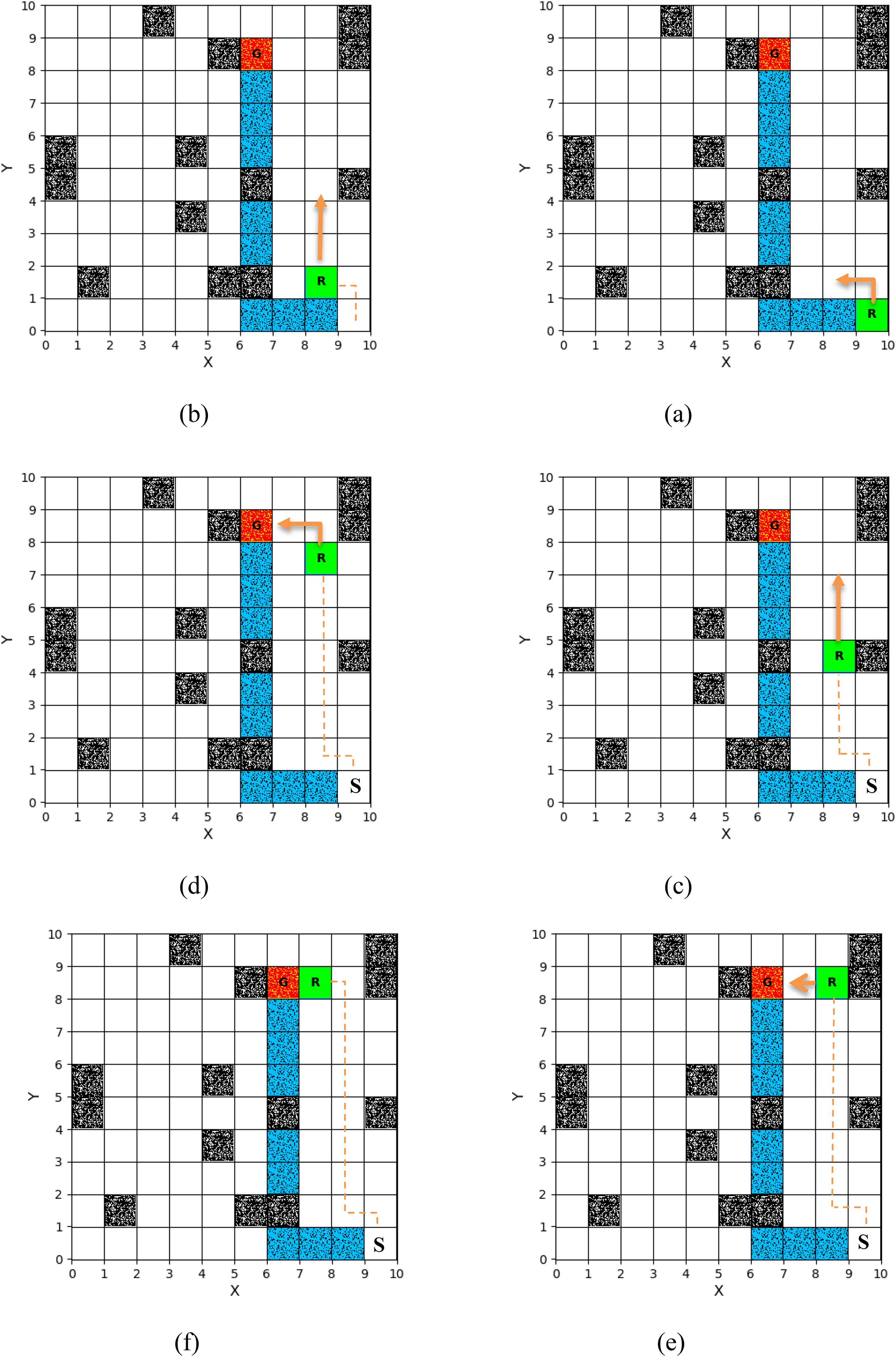
Agent navigating Figure 8 towards the goal in the second scenario, test two: (a) first step, (b) third step, (c) seventh step, (d) 10th step, (e) 11th step, (f) 12th step.

Test 2

In the second test (Figure 7), the agent operated in a 20 × 20 environment containing 40 static obstacles. Despite the limited path availability and the proximity of the goal to multiple obstacles, the agent utilized adaptive decision-making to identify a safe, optimal path without collisions. The results demonstrate the algorithm's capability to navigate dense environments by selecting the shortest path from the starting point.

Figure 7.

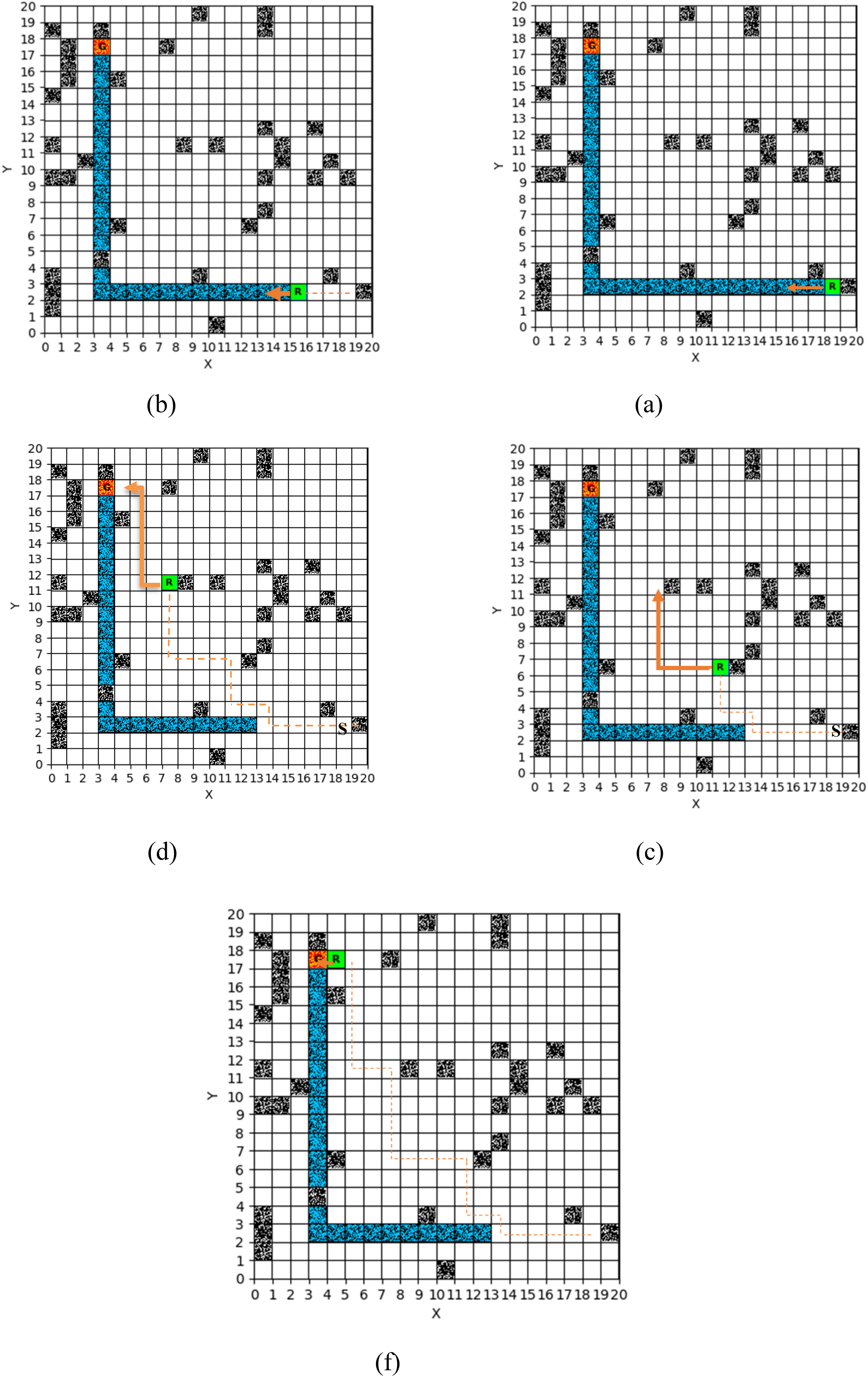
Third test in a 20 by 20 environment: (a) first step; (b) sixth step; (c) 13th step; (d) 20th step; (e) 30th step.

Testing in the 3D environment of ROS2

To assess network performance under realistic and spatially intricate conditions, a 3D robot simulation was conducted using the ROS2 platform (Humble Hawksbill release) on Ubuntu 22.04 LTS. As an advanced iteration of ROS1, ROS2 is considered suitable for testing navigation algorithms in complex environments due to its distributed architecture, real-time capabilities, and compatibility with modern tools. The Gazebo Classic simulator was employed to enable visualization and interaction with the environment. As shown in Figure 8, the TurtleBot3 Burger mobile robot model was integrated into ROS2 via the official turtlebot3_gazebo package. This package contains URDF files that define the robot's geometry, joints, and sensors, as well as SDF files for the physical settings within the Gazebo environment. To emphasize lidar-based navigation, peripheral sensors such as the RGB camera and the inertial measurement unit (IMU) were removed from the model, thereby reducing the computational load of the simulation. Communication between the learning agent and the environment was facilitated through the rclpy library. The agent was defined as an independent node in ROS, which received lidar sensor data (/scan) and positional data (/odom) through a Subscriber, while sending movement commands to the /cmd_vel Topic via a Publisher. The main nodes included turtlebot3-diff-drive, turtlebot3-laserscan, turtlebot3-joint-state, and turtlebot3-imu, which transmitted relevant data to the robot-state-publisher and turtlebot3-dqn nodes.

Figure 8.

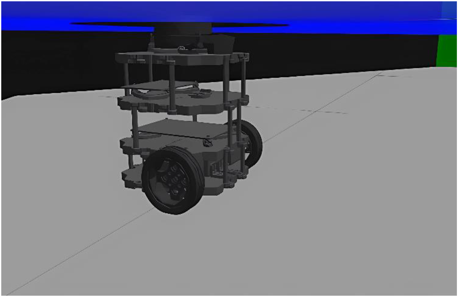
TurtleBot3 burger robot simulated in a Gazebo environment.

The turtlebot3-dqn node processed this data and generated actions for the agent. The frequency for receiving sensor data and executing agent actions was set to the default settings of ROS and Gazebo, approximately 10 Hz for observations and a decision cycle of 0.5 s. The robot's state and the path it traveled were displayed using the Gazebo tool. This modular simulation structure can be reproduced and expanded for multi-agent scenarios. It is important to note that the experiments conducted in this study were limited to static environments with fixed obstacles. Future research will focus on developing the proposed method for dynamic environments that include moving obstacles. This advancement will allow for a more comprehensive assessment of the algorithm's performance under realistic conditions and enhance its applicability in more complex scenarios.

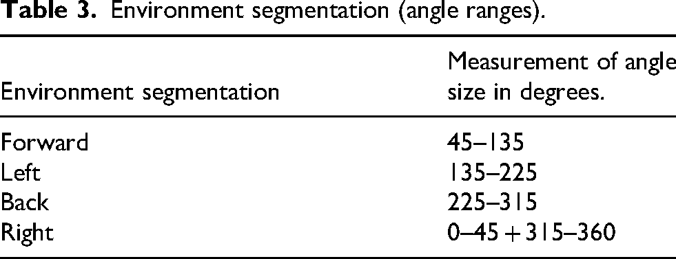
The technical specifications of the lidar sensor are fully detailed in Table 3, with additional information about both the lidar sensor and the loaded robot provided in the appendix. Initially, the robot could only determine its position based on the four cardinal directions. To improve this, precise angle segmentation was used to define the directions of movement. Angles were organized into a table for clarity. Additionally, the distance to the nearest obstacle in each direction was measured using the lidar sensor, which served as a crucial input for developing the robot's movement strategy.

Table 3.

Environment segmentation (angle ranges).

Environment segmentation	Measurement of angle size in degrees.
Forward	45–135
Left	135–225
Back	225–315
Right	0–45 + 315–360

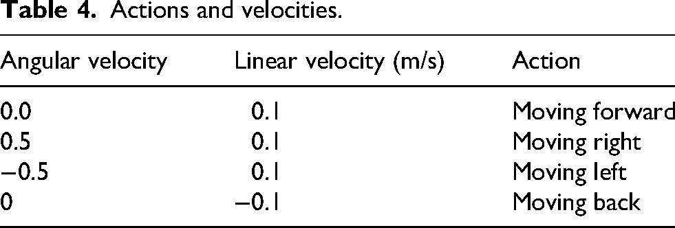
The robot operates in a continuous environment that is divided into a square grid to enhance processing and improve sampling accuracy. This model features grid dimensions of 200 × 200, with each cell separated by a distance of 0.1 units. The robot's actions are categorized into four main types, each defined by specific linear and angular velocity characteristics. Table 4 summarizes these actions.

Table 4.

Actions and velocities.

Angular velocity	Linear velocity (m/s)	Action
0.0	0.1	Moving forward
0.5	0.1	Moving right
−0.5	0.1	Moving left
0	−0.1	Moving back

A tree diagram is presented to illustrate the communication structure of the nodes surrounding vertex 2.

In this diagram (Figure 9), each node is represented as either a circle or a rectangle, while the connecting lines depict the parent–child relationships and data exchange pathways. This graphical representation is designed to clearly demonstrate the branching paths of the nodes originating from the central vertex (with the value 2) and the angular layout of each section. main nodes are responsible for sending and receiving data, collectively forming the overall structure of the network. The Gazebo simulation results in Figure 10 demonstrate the robot's progression from the starting position (a) through the environment (b) until reaching the goal (c).

Figure 9.

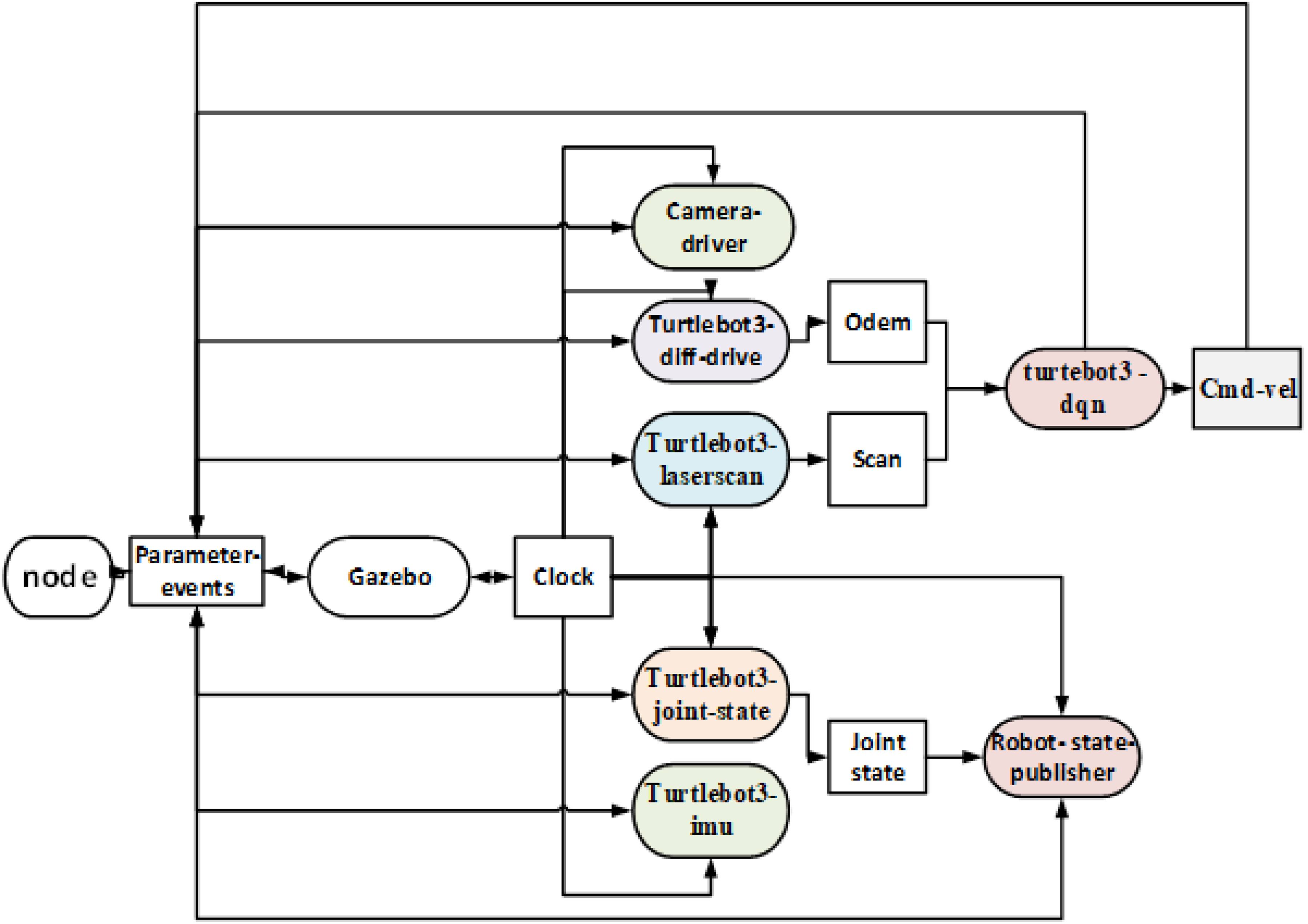
How the various components of RAS2 communicate.

Figure 10.

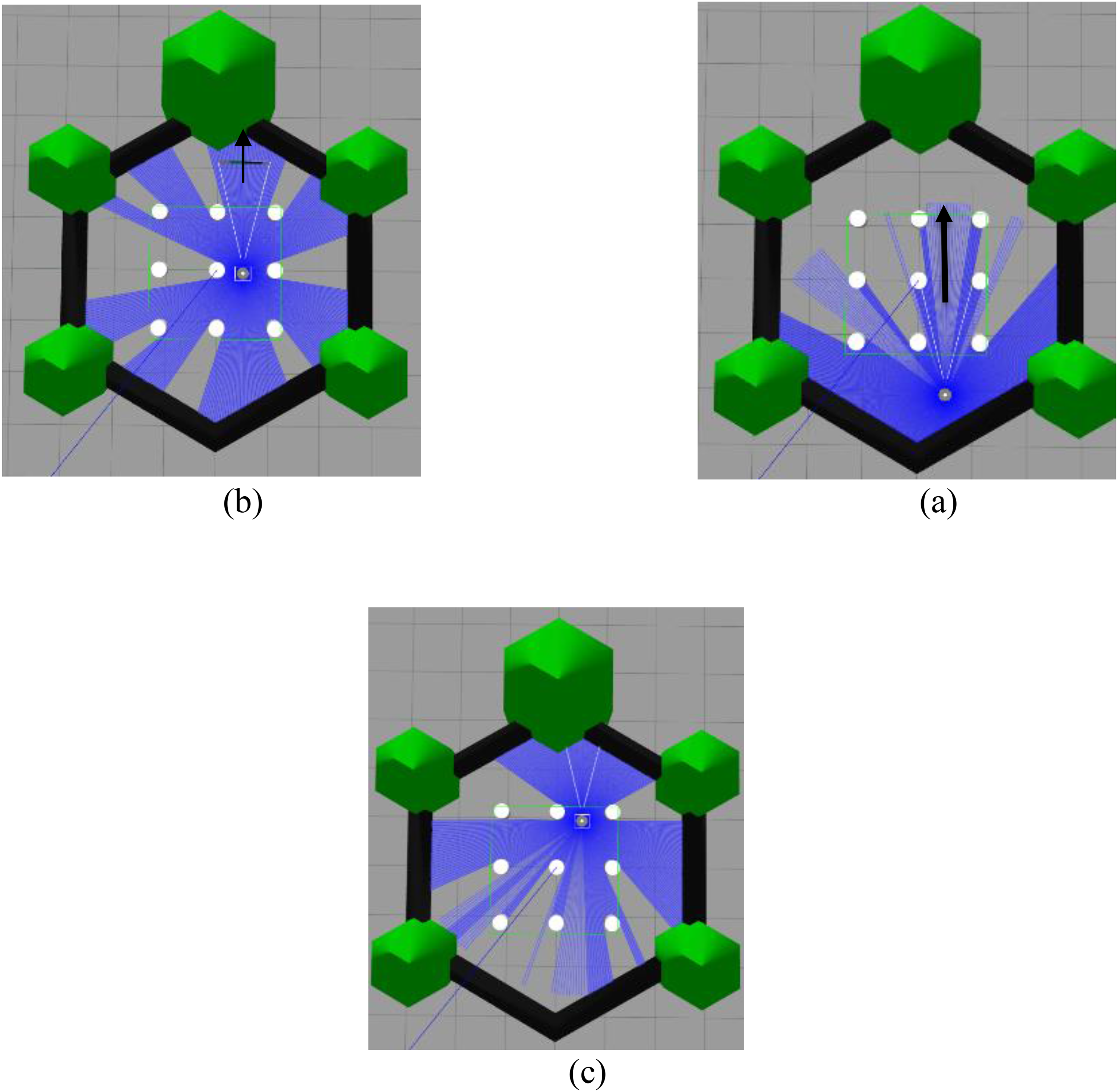
Schematic movement of the robot from (a) the starting point, (b) on the way to the goal, to (c) reaching the goal.

In the second scenario, depicted in Figure 11, the objective was to assess the robot's ability to navigate to a specific point in the corner of the screen. Since the target position is located in the left corner of the environment, the robot primarily performs forward and leftward movements to reach its destination in the most efficient manner

Figure 11.

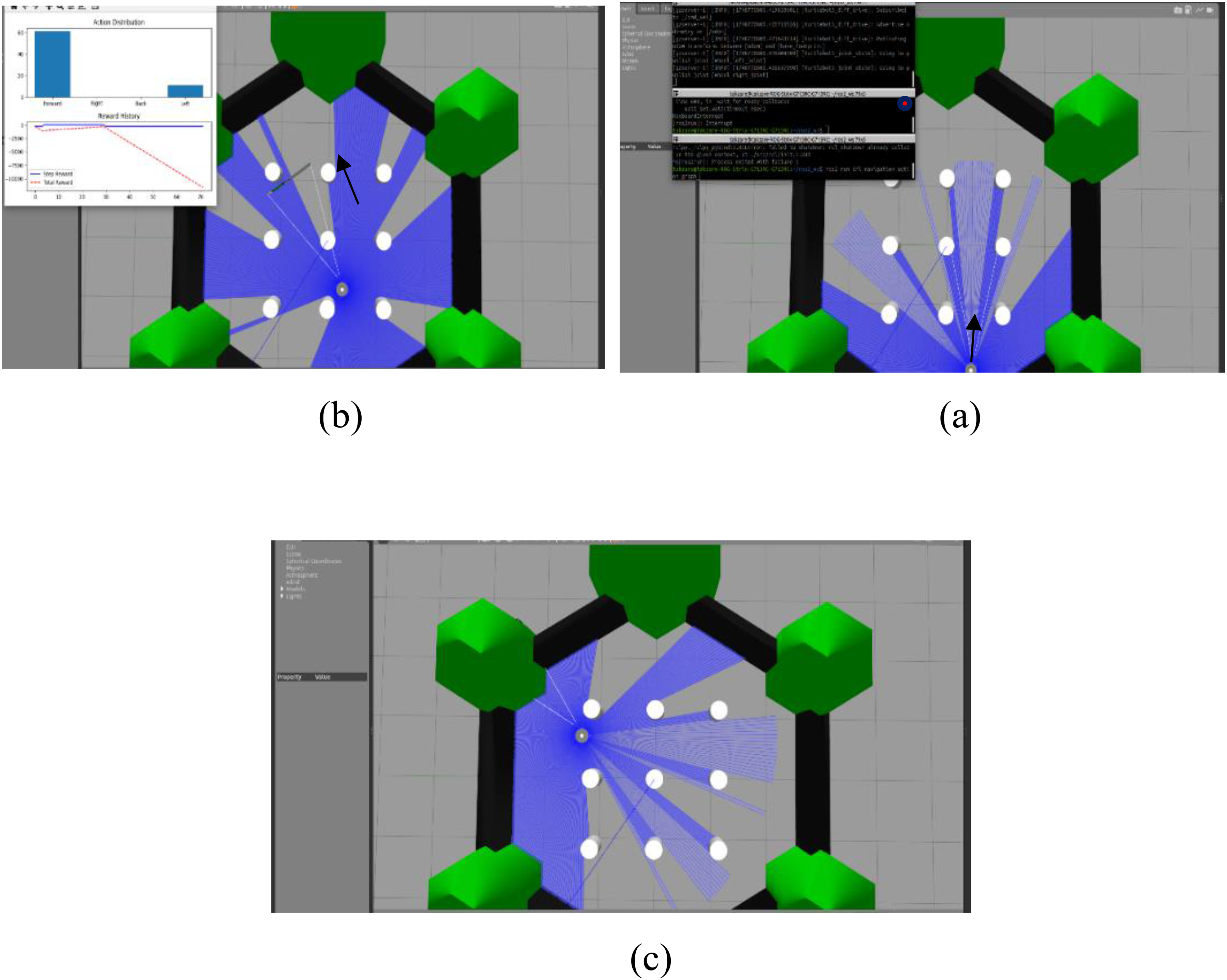
Schematic of the robot's movement: (a) from the starting point, (b) around the obstacle, and (c) reaching the goal.

Navigation for mobile robot

The robot has a maximum translational speed of 0.22 m/s and a maximum rotational speed of 162.72°/s. In Figure 12, a view of the robot is presented. To conduct real experiments using the Turtle 2 robot, the trained agent algorithm is directly implemented on the robot, meaning that the trained neural network weights are loaded into the robot from a stored file. The multi-stage priority network of the dual Q-network receives the current state as input and produces Q-values for all possible actions as output.

Figure 12.

Robot used for experimental tests.

The general state space described in Section 2.5 is represented as a vector with the feature (1, 10). This state vector contains normalized distances between the robot and its surroundings, measured in four sectors using the robot's lidar sensor. The lidar sensor operates at a rotation frequency of 5 Hz, but only four measurements are selected. For distances greater than 100 divided cells (the diameter of the sensing area), the corresponding value is set to 1. The full power is normalized by dividing by the diameter of the sensing area (R). This vector is then fed into the trained network of the proposed algorithm. The network generates Q-values corresponding to four possible actions. The action with the highest Q-value is selected and sent to the robot for execution. As previously mentioned, the lidar sensor has a rotation frequency of 5 Hz, meaning it takes 200 ms to scan the entire sensory area, including all sectors. This duration is necessary to form a state, as the computation time is considered negligible. The episode execution process continues until one of the following conditions is met: (1) reaching the target, indicated by the robot being less than a predetermined threshold distance (0.5 m) from the target; (2) colliding with an obstacle, defined as the robot being less than a critical distance (0.3 m) from any obstacle in the environment at any point during the episode; or (3) exceeding the maximum number of actions allowed, which is set at 1200 actions per episode.

Preparing the initial testing environment

The process of simultaneous localization and mapping (SLAM) is a fundamental component of autonomous navigation systems. It enables robots to accurately navigate and comprehend the structure of unknown environments. To evaluate the performance of the algorithms used under non-static conditions, the robot was placed in an unfamiliar setting featuring artificial structures such as designed walls, as illustrated in Figure 13, To aid in the localization and mapping process, the “graph-based mapping” software package was utilized. This software is designed to create a comprehensive map of the environment using data collected from sensors. During this phase, the robot was manually maneuvered through the test space while crucial data was gathered via an optical rangefinder sensor. This dataset is vital because it allows the robot to determine its location and understand the spatial arrangement of the environment. In this scenario, the robot navigates within an environment that contains static obstacles. Two linear obstacles are positioned in the robot's initial path, and the final destination is marked with a cross symbol. Despite being relatively surrounded by obstacles, the robot must identify a suitable route to reach the goal. This experiment is intended to assess the robot's ability to recognize navigable paths and make decisions under constrained conditions.

Figure 13.

First scenario of the experimental test (a) beginning of the path in the real environment; (b) beginning of the path at the ros; (c) approaching the obstacle in the real environment; (d) approaching the obstacle at the ros; (e) bypassing the obstacle in the real environment; (c) bypassing the obstacle in the ros; (h) reaching the goal in the real environment; (k) reaching the goal at the ros.

Ten evaluation criteria

The proposed structure is thoroughly and comparatively assessed alongside existing methods using the evaluation framework introduced in.³³ This framework (Table 5) consists of ten performance criteria, each representing a critical aspect of the design and implementation of path planning and obstacle avoidance algorithms in both simulated and real-world environments. In this evaluation, each method that meets a criterion is awarded one point. The total points accumulated serve as an indicator of the method's comprehensiveness and efficiency. The criteria being evaluated are:

Table 5.

Definition of performance criteria.

Code	Criterion
DSSO	Diverse size and shape obstacles
MO	Multiple obstacles
CSG	Configurable start and goal
ALM	Avoidance of local minima
DEN	Explicit representation needed
CC	Computational cost
RTP	Real-time planning
EC	Environmental complexity
S	Scalability
PPPOA	Parallel path planning and obstacle avoidance

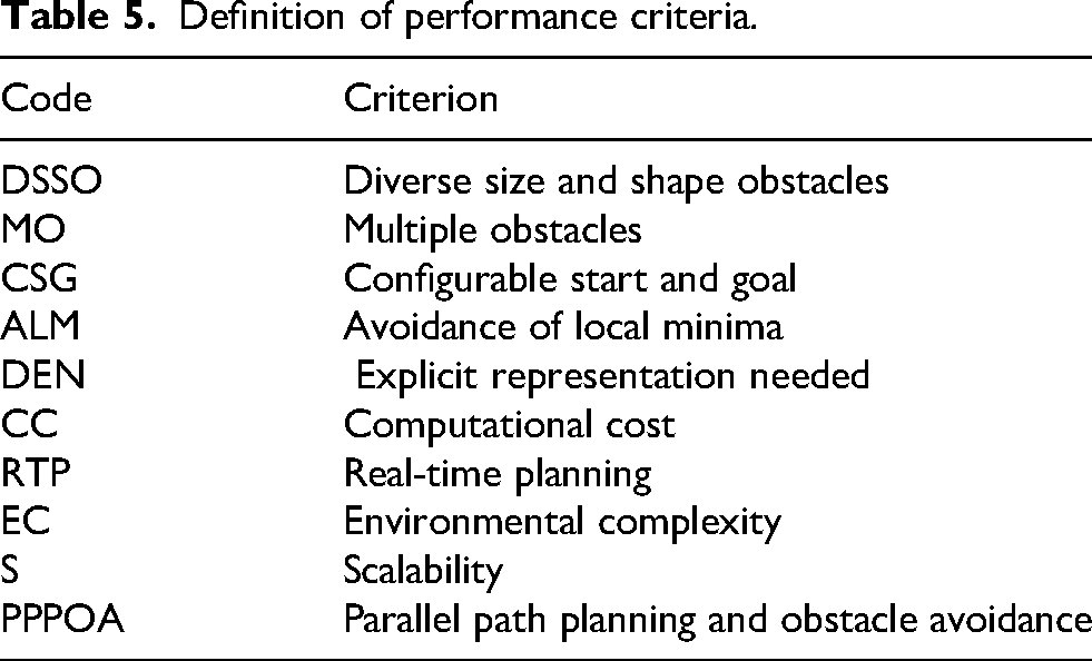
Table 6 compares the proposed structure with six selected methods from the research literature. A “+” indicates that the criterion is met by the corresponding method, while a “–” indicates that it is not met. The proposed structure, denoted by “US”, has achieved a full score in all categories.

Table 6.

Comparison of the proposed structure based on performance criteria.

	DSSO	MO	CSG	ALM	DEN	CC	RTP	EC	S	PPPOA	FA
³⁴	1	1	0	1	1	0	0	0	0	0	4
³⁵	0	0	1	1	1	1	1	0	0	0	5
³⁶	0	1	1	1	1	0	0	0	1	1	6
³⁷	0	1	1	1	0	1	1	0	1	0	7
³⁸	1	1	1	0	1	1	1	0	1	1	8
³⁹	1	1	1	1	1	1	1	0	0	1	8
⁴⁰	1	1	1	1	1	1	1	0	1	1	9
US	1	1	1	1	1	1	1	1	1	1	10

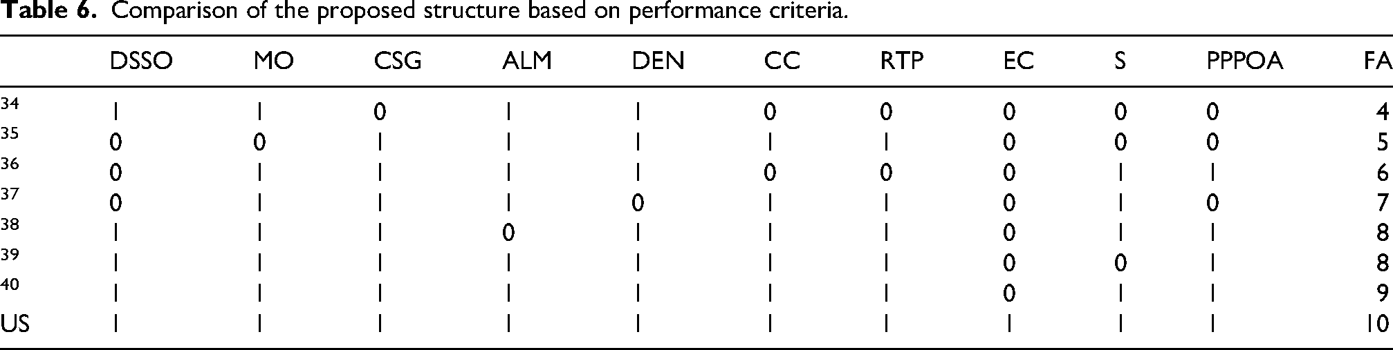
In summary, the ten structural criteria in Table 6 directly drive the superior performance of PER-MS-DDQN, serving as the technical differentiator from existing literature.^34–40 Stability is ensured by the integration of environmental complexity (EC), scalability (S), multiple obstacles (MO), and diverse shapes (DSSO)—parameters notably absent in³⁴ and³⁶—resulting in a 43% lower standard deviation and consistent episode durations across complex maps. Convergence is accelerated by the avoidance of local minima (ALM), low computational cost (CC), and lack of explicit representation (DEN). By building upon the efficiency frameworks of,^35,37 our architecture achieves a 35% shorter training duration and 65% faster processing, confirmed by the narrowing Q1–Q2 gap. Finally, the 99% success rate is the direct outcome of real-time planning (RTP), parallel path planning (PPPOA), and configurable start/goals (CSG). While high-performing models like^38,39 satisfy eight criteria, and the state-of-the-art in⁴⁰ satisfies 9, only our 10/10 architectural design provides the full mechanical redundancy to improve from an initial 38% to a final 99% reliability. This synthesis confirms that satisfying the complete set of ten criteria is the fundamental driver of the algorithm's stability and efficiency.

Conclusion

In this paper, a hybrid PER–MS–DDQN algorithm was introduced and evaluated to enhance the navigation of mobile robots in unknown environments. The core contributions of the approach involved creating a multilayered observation space, utilizing angular segmentation of movements, discretizing the environment, and integrating lidar sensor inputs to develop an accurate model for understanding the surroundings. The algorithm featured a hybrid reward structure that combined cumulative and staged rewards, along with an action selection framework based on the maximum ergium criterion. This enabled more intelligent decision-making in complex situations.

Experimental results confirm that PER-MS-DDQN significantly outperforms the baselines, achieving an average final reward of 345 units (a 23% improvement over the competitive method (280 units) and up to 12 times better than the baseline DDQN). The proposed method achieved a 99% final success rate while reducing reward volatility by 40% and standard deviation by up to 43% compared to DDQN. Furthermore, the algorithm demonstrated high efficiency with an average processing speed of 7 s (a 65% reduction compared to 20 s for PER-DDQN) and a 35% increase in training speed. These numerical indicators provide evidence of the accelerated convergence, higher stability, and significant generalizability of PER–MS–DDQN in diverse environments.

However, a limitation of the current algorithm is its reduced efficiency in highly dynamic environments with fast-moving obstacles. Future research will focus on addressing these limitations by integrating temporal state representations and testing the framework in real-world dynamic scenarios.

Footnotes

ORCID iDs

Moharam Habibnejad Korayem

Niloufar Takzare

Funding

The authors received no financial support for the research, authorship, and/or publication of this article.

Declaration of conflicting interests

The authors declared no potential conflicts of interest with respect to the research, authorship, and/or publication of this article.

References

Xiao

Liu

Warnell

, et al. Motion planning and control for mobile robot navigation using machine learning: a survey. Auton Robots 2022; 46: 569–597.

Chang

Shan

Jiang

, et al. Reinforcement based mobile robot path planning with improved dynamic window approach in unknown environment. Auton Robots 2021; 45: 51–76.

Korayem

Kia

Lademakhi

. Intelligent saturation power limit load distribution algorithm (ISPLLDA) for cooperative manipulators applications. J Intell Rob Syst 2025; 111: 15.

Zou

Xiong

Hou

. An end-to-end learning of driving strategies based on DDPG and imitation learning. In: 2020 Chinese control and decision conference (CCDC), 2020. IEEE, pp.3190-3195.

Chu

Sun

Zhu

, et al. Motion control of unmanned underwater vehicles via deep imitation reinforcement learning algorithm. IET Intel Transport Syst 2020; 14: 764–774.

Liu

Dugas

Cesari

, et al. Robot navigation in crowded environments using deep reinforcement learning. In: IEEE/RSJ international conference on intelligent robots and systems (IROS), 2020. IEEE, pp.5671-5677.

Toan

Woo

. Mapless navigation with deep reinforcement learning based on the convolutional proximal policy optimization network. In: IEEE international conference on big data and smart computing (BigComp), 2021. IEEE, pp.298-301.

Wang

Esfahani

, et al. Learn to navigate autonomously through deep reinforcement learning. IEEE Trans Ind Electron 2021; 69: 5342–5352.

Shinde

Shah

. A review of machine learning and deep learning applications. In: 2018 Fourth international conference on computing communication control and automation (ICCUBEA), 2018. IEEE, pp.1-6.

10.

Kato

Morioka

. Autonomous robot navigation system without grid maps based on double deep Q-network and RTK-GNSS localization in outdoor environments. In: 2019 IEEE/SICE international symposium on system integration (SII), 2019. IEEE, pp.346-351.

11.

Zhang

Gai

Zhang

, et al. Double-DQN based path smoothing and tracking control method for robotic vehicle navigation. Comput Electron Agric 2019; 166: 104985.

12.

Sun

Zhai

Qin

. Crowd navigation in an unknown and dynamic environment based on deep reinforcement learning. IEEE Access 2019; 7: 109544–109554.

13.

Zhang

Liu

. Danger-aware adaptive composition of drl agents for self-navigation. Unmanned Syst 2021; 9: –9.

14.

Wang

Schaul

Hessel

, et al. Dueling network architectures for deep reinforcement learning. In: International conference on machine learning, 2016. PMLR, pp.1995-2003.

15.

Hua

Zeng

, et al. Learning for a robot: deep reinforcement learning, imitation learning, transfer learning. Sensors 2021; 21: 1278.

16.

Peng

Chen

Zhang

, et al. Enhanced autonomous navigation of robots by deep reinforcement learning algorithm with multistep method. Sens Mater 2021; 33: 1–18.

17.

Bin Issa

Das

Rahman

, et al. Double deep Q-learning and faster R-cnn-based autonomous vehicle navigation and obstacle avoidance in dynamic environment. Sensors 2021; 21: 1468.

18.

Brittain

Bertram

Yang

, et al. Prioritized sequence experience replay. arXiv preprint arXiv:1905.12726, 2019.

19.

Dan

Quan

Budden

. Distributed prioritized experience replay. arXiv preprint arXiv:1803.00933, 2018.

20.

Zhu

, et al. An improved dueling deep double-q network based on prioritized experience replay for path planning of unmanned surface vehicles. J Mar Sci Eng 2021; 9: 1267.

21.

Shuhai

Shangjie

Cun

. Path planning for outdoor mobile robots based on IDDQN. IEEE Access 2024; 12: 51012–51025.

22.

Zhang

Shi

Zhang

, et al. A DDQN path planning algorithm based on experience classification and multi steps for mobile robots. Electronics (Basel) 2022; 11: 2120.

23.

Yang

Huang

Wang

, et al. High-speed three-dimensional aerial vehicle evasion based on a multi-stage dueling deep Q-network. Aerospace 2022; 9: 73.

24.

Mnih

Kavukcuoglu

Silver

, et al. Human-level control through deep reinforcement learning. nature 2015; 518: 529–533.

25.

Xue

Zhang

, et al. A deep reinforcement learning method for mobile robot collision avoidance based on double dqn. In: 2019 IEEE 28th international symposium on industrial electronics (ISIE), 2019. IEEE, pp.2131-2136.

26.

Xie

Shao

, et al. Deep reinforcement learning with optimized reward functions for robotic trajectory planning. IEEE Access 2019; 7: 105669–105679.

27.

Kashyap

Konathalapalli

. Autonomous navigation of ROS2 based Turtlebot3 in static and dynamic environments using intelligent approach. Int J Inf Technol 2025: 1–23.

28.

Escobar-Naranjo

Caiza

Ayala

, et al. Autonomous navigation of robots: optimization with DQN. Appl Sci 2023; 13: 7202.

29.

Cai

Sun

, et al. Autonomous navigation by mobile robot with sensor fusion based on deep reinforcement learning. Sensors 2024; 24: 3895.

30.

Hossain

Doukhi

, et al. Deep reinforcement learning-based ros-controlled rc car for autonomous path exploration in the unknown environment. In: 2020 20th International conference on control, automation and systems (ICCAS), 2020, pp.1231-1236.

31.

Lin

, et al. Federated reinforcement learning framework for mobile robot navigation using ROS and gazebo. IEEE Internet Things Mag 2025. DOI: 10.1109/MIOT.2025.3575929

32.

Alapati

Prakash

. Autonomous navigation of turtleBot3 using DDPG reinforcement learning in ROS2 framework. In: International conference on sustainable communication networks and application (ICSCNA), 2024. IEEE, pp. 1356-1361.

33.

Yasin

Mohamed

Haghbayan

M-H

, et al. Unmanned aerial vehicles (uavs): collision avoidance systems and approaches. IEEE Access 2020; 8: 105139–105155.

34.

Mirowski

Pascanu

Viola

, et al. Learning to navigate in complex environments. arXiv preprint arXiv:1611.03673, 2016.

35.

Duguleana

Mogan

. Neural networks based reinforcement learning for mobile robots obstacle avoidance. Expert Syst Appl 2016; 62: 104–115.

36.

Wang

Liu

, et al. Mobile robot path planning in dynamic environments through globally guided reinforcement learning. IEEE Rob Autom Lett 2020; 5: 6932–6939.

37.

Xia

El Kamel

. Neural inverse reinforcement learning in autonomous navigation. Rob Auton Syst 2016; 84: 1–14.

38.

Jin

Wang

. Proximal policy optimization based dynamic path planning algorithm for mobile robots. Electron Lett 2022; 58: 13–15.

39.

Cheng

W-C

Zhong

, et al. Autonomous robot goal seeking and collision avoidance in the physical world: an automated learning and evaluation framework based on the ppo method. Appl Sci 2024; 14: 11020.

40.

Quan

Zhang

. A novel mobile robot navigation method based on deep reinforcement learning. Int J Adv Rob Syst 2020; 17: 1729881420921672.

Enhanced navigation for mobile robots in unknown environments using PER-DDQN with multi-step techniques

Abstract

Keywords

Introduction

Theoretical foundations and associated algorithms

Reinforcement learning

DQN and DDQN algorithms

Priority experience reply memory

Proposed algorithm

Designing an enhanced viewing environment for robot navigation

Proposed reward function

Training and testing

Network training process

Grid world

Mobile robot network and navigation training

Testing in grid worlds

Test 1

Test 2

Testing in the 3D environment of ROS2

Navigation for mobile robot

Preparing the initial testing environment

Ten evaluation criteria

Conclusion

Footnotes

ORCID iDs

Funding

Declaration of conflicting interests

References