Sage Journals: Discover world-class research

Abstract

Mobile robots that operate in real-world environments need to be able to safely navigate their surroundings. Obstacle avoidance and path planning are crucial capabilities for achieving autonomy of such systems. However, for new or dynamic environments, navigation methods that rely on an explicit map of the environment can be impractical or even impossible to use. We present a new local navigation method for steering the robot to global goals without relying on an explicit map of the environment. The proposed navigation model is trained in a deep reinforcement learning framework based on Advantage Actor–Critic method and is able to directly translate robot observations to movement commands. We evaluate and compare the proposed navigation method with standard map-based approaches on several navigation scenarios in simulation and demonstrate that our method is able to navigate the robot also without the map or when the map gets corrupted, while the standard approaches fail. We also show that our method can be directly transferred to a real robot.

Keywords

Mobile robotics reinforcement learning navigation deep learning

Introduction

Intelligent machines should be able to perform complex tasks in unstructured environments. Moreover, they should be able to operate in a safe manner, avoiding possible damages to the environment, other agents, or themselves. For mobile robots, this requirement implies a need for a navigation system, performing obstacle avoidance and path planning.

In static environments, the standard approach is to build a map of the environment and deploy a localization system along with a path-planning algorithm and control system to safely navigate the robot in the environment. However, for certain navigation tasks, we might want the robot to be immediately operational in a new environment, while in other environments the rate of change of the surroundings might make preserving a valid map infeasible (e.g. a robot moving in a crowded area, exposition spaces where equipment and furniture are frequently displaced, a robot in a marina). For these types of environments, where using a map is impractical, it can be more appropriate to develop a map-less navigation approach, relying on the current sensor readings without an explicit map.

We state our problem as the task of navigating a mobile robot to a given goal location, specified in terms of bearing and distance from the current robot pose, without having any a priori information about the environment. We assume that the environment is partially observable using the robot sensors and that the distance and bearing are continuously obtainable. Driven by the progress of reinforcement learning (RL) methods in recent years, along with the principal suitability of applying RL to an agent sequentially interacting with an environment, we develop a new method for creating map-less and goal-driven navigation RL policies. Our navigation policies operate in an iterative process of taking an observation of the world, in the form of a laser range scan along with the distance and angle to the goal and generating a velocity command for the robot. Building on our previous work,¹ we first consider the problem of navigation as a Markov decision process² (MDP) and then implicitly as a partially pbservable Markov decision process³ (POMDP) and optimize a navigation policy modeled by a deep neural network in the framework of RL, specifically with an approach based on the state-of-the-art A2C⁴ method as visualized in Figure 1.

Figure 1.

Summary of our approach: Navigation policy learned in simulation using deep reinforcement learning and applied to a real robot.

Training neural networks on experience generated by real robots is costly, as batteries require recharging, resetting experiments requires manual effort, and physical components can be worn down and require maintenance. These problems are exacerbated when learning navigation policies for mobile robots since there is the added difficulty of acquiring negative samples, which are mostly collisions. Additionally, most RL algorithms depend on large quantities of samples for training. The required amount of samples can be produced either by using multiple robots (difficult when working with mobile robots), training in a really authentic simulator, or training in somewhat abstracted simulator but managing to regularize the samples by performing considerable randomization in the simulation parameters, which is what we do in our approach.

The main contribution presented in this article is a novel reactive local navigation method for steering the robot to global goals without relying on a map of the environment. The proposed navigation model is trained in a deep RL framework and is able to directly translate robot observations to movement commands. We implement the trained policies on a robot with a 2D laser range scanner and evaluate their performance on various navigation tasks in a polygon of obstacles. The results show that as the map gets corrupted, our approach outperforms global navigation methods.

In the following section, we present the related work. In the Approach section, we present in detail our proposed method. This is followed by the section describing the experiment setup and evaluation results. In the last section, we present our conclusions.

Related work

Model-free methods for optimizing MDPs make it possible to find an optimal policy without explicitly modeling the dynamics of the underlying MDP. Q-learning⁵ and methods based on Policy Gradients⁶ are among the most significant such methods.

Recently, incredible results were presented by Mnih et al.⁷ by their deep Q-networks (DQN), where they achieved a human level performance on a number of Atari games. Wang et al.⁸ applied the same optimization algorithm but designed a novel network architecture, separating the state-values, and the action-advantages named Dueling DQN. This architecture beat the state of the art on the Atari benchmark. Then van Hasselt et al.⁹ presented a method named Double DQN which uses a second, target Q-network, and so circumventing the maximization bias in Q-learning and achieving better results in a number of domains. The training of these deep models is made practically viable by employing methods of experience replay¹⁰ like Prioritized Experience Replay developed by Schaul et al.¹¹ Employing experience replay significantly speeds up the convergence of the network by breaking down the high correlation between successive samples.

While policy gradients have been around for quite some time, Mnih at al. developed the Asynchronous Advantageous Actor Critic (A3C) method⁴ for a neural network implementation of a policy function that outperforms the standard DQN, on some games also the Double DQN and in numerous experiments demonstrated the superiority of policy gradient methods for some classes of problems. In parallel methods like the Trust Region Policy Optimization,¹² Proximal Policy Optimization¹³ and Deep Deterministic Policy Gradients¹⁴ were also developed, providing some improvements to the convergence properties and faster learning in some situations scenarios.

The first experiments in learning a navigation policy with RL were done before the mass adoption of neural networks, using tables for approximating the policy or value functions. This was mostly done by severe discretization of the state space. Adbel et al.¹⁵ implement a tabular form of Q-learning for obstacle avoidance and assume a fully observable environment. A fully observable environment is often not available to a robot, and the tabular Q-learning can only be applied up to a certain environment-complexity, as the method suffers from the curse of dimensionality. Konar et al. developed Improved Q-learning (IQL)¹⁶ as an extension of Extended Q-learning¹⁷ and applied it to path-planing in an environment represented by a grid. The IQL algorithm presupposes a knowledge of the distance to the next-state (observation) which is not always available. Wen et al.¹⁸ used a tabular implementation of the Q-learning algorithm merged with EKF-SLAM¹⁹ for an obstacle avoidance system on an NAO robot. They use clustering methods to preprocess the laser-scan data.

The availability of computing hardware and development of efficient techniques for training deep networks has made possible the circumvention of some of the negative effects of drastic discretization—using powerful neural networks to approximate the state-value function, Q-function, or directly the policy. Gupta at el.²⁰ implemented an end-to-end system for learning simultaneous mapping and planning for robotic navigation by applying a value iteration method. This method in general converges slower than either Q-learning or policy-gradient methods. A variant of Q-learning (fitted Q iteration) was applied to an in-simulation learning system,²¹ which through high randomization can to a certain degree of success, be directly applied to the target domain. In our work, we use the policy gradient method A2C and use recurrent long short-term memory (LSTM) units in the structure of our policy network. The main differences to other work in RL is the treatment of the goal as a part of the state, and especially the design of the output layers, where we split the output layer of the LSTM unit into two separate streams which we optimize within the same loss function, by summing the two losses, and jointly updating the parameters.

Recently, a lot of “deep” methods have focused on navigation based on camera input. Xie et al.²² have developed a monocular image obstacle avoidance method based on the dueling and double-Q mechanisms. This method however does not navigate to a goal location. Bruce et al.²³ present a method based on DQN for navigation based on a 360° camera mounted on a robot, but to a fixed location in a previously known environment. By adding auxiliary losses to the A3C algorithm and using additional techniques, Mirowski et al.²⁴ manage to train an agent for navigation in a virtual maze environment. Zhu et al.²⁵ developed a method for navigating to a target given as an image in a previously known environment; however, this approach is not applicable to navigation in an unknown environment, especially as the policy uses scene specific layers in its structure. Kulahanek et al.²⁶ took this idea further by removing the scene specific layers and using ideas of training with auxiliary tasks for learning better feature extraction from the image. Leiva et al.²⁷ train a collision policy which as input combines the date from the RGB, depth image, and lasers on the robot.

We consider our work parallel to these work, since our navigation policy as the main input takes only a laser-scan rather than an RGB or a depth image. Additionally, unlike in previous studies,^25,26 our algorithm assumes that the robot operates in continuous space and does not deterministicly move by a certain distance in a given direction. Taking this in consideration, our policy can be applied on many existing robots without making any changes in their hardware and without incurring additional integration costs.

The work most closely related to ours is Tai et al.²⁸ They also train a navigation policy for the TurtleBot using a Deep RL algorithm. In their approach, they use the deterministic policy gradient algorithm, while our work is based on the A2C method. Additionally, we use a simpler simulator for training and are able to generate samples faster, we provide greater randomization by permuting the obstacles and starting positions at each trial which we expect to translate to better applicability to unseen environments. The most significant contribution is the integration of a recurrent network in the navigation policy which implicitly addresses the partial observability of the problem.

Approach

In this section, we present in short the RL framework, and then the A2C method for solving RL problems. Then we formulate robot navigation as a RL problem, present the proposed neural networks, and explain in detail the procedure for training them.

Reinforcement learning

Put in the most general terms, in RL, we try to discover a policy of acting so as to maximize a certain reward signal, just by interacting with a given environment. We interact with the environment in iterations and in each iteration we receive an observation and a reward and we produce an action that is sent to the environment. This process of interacting can end by encountering a terminal state or the process can continue forever.

The process we are interacting with is usually formalized as an MDP if we assume that the observation we get at each time step fully describes the state of the environment, or it can be formalized as a POMDP if we assume that the underlying state is hidden. If we do not try to learn a model of the process during this interaction, we are working with model-free RL, as the majority of recent successes in RL. We formulate the task of navigation first as an MDP and later as a POMDP.

An MDP is defined by a set of states S, a set of actions A, transition function $t (s, a) : S \times A \mapsto S$ (or if the process is stochastic $t (s, a) : S \times A \mapsto P r (S)$ ), a reward at each time-step R_k, and a discount factor for the future rewards $γ \in [0, 1]$ . The agent is randomly initialized in the environment, after which it observes the state s₀ and performs an action a₀ according to a deterministic policy $π (s) : S \mapsto A$ , or stochastic policy $π (a | s) : A \times S \mapsto ℝ$ . This takes the agent to the state s₁ and it receives a reward of R₁. This process continues iteratively until a terminal state is reached or it continues forever. The MDP framework is quite general and a lot of problems can be formalized within it. However, in some problems, the observation that we get from the environment does not contain the complete information about the current state, which we need for making optimal decisions. Sometimes we can still learn useful policies by treating the underlying partially observable problem as a fully observable problem. In general, to model such problems more accurately, we usually use the framework of POMDP.

A POMDP is defined by a tuple $〈 S, A, T, R, γ, Ω, O 〉$ , where S is a set of states, A is a set of actions, $T : S \times A \to Pr (S)$ is a state-transition function which gives the probability that we end up in state $s^{'}$ if we take action a in state s ( $T (s, a, s^{'}) = Pr (s^{'} | s, a)$ ), $R : S \times A \to ℝ$ is a reward the agent receives at each time-step for taking a certain action in a certain state, $γ \in [0, 1]$ is a discount factor, $Ω$ is a set of observations that the agent can experience, and $O : S \times A \to Pr (Ω)$ is an observation function which gives the probability for experiencing the observation o if the agent took action a and ended up in state $s^{'}$ ( $O (s^{'}, a, o) = Pr (o | s^{'}, a)$ ).

Optimization

Let G_t be the total sum of discounted rewards, going from time t forward: $G_{t} = R_{t + 1} + γ R_{t + 2} + \dots = \sum_{k = 0}^{k_{final}} γ^{k} R_{t + k + 1}$ . Now we can define the state-value function as $V_{π} = E [G_{t} | S_{t} = s]$ , or in plain words, the total expected return, given that we are currently in state s and are following policy $π$ . Similarly, we can also define the action-value function as $Q_{π} = E [G_{t} | S_{t} = s, A_{t} = a]$ which can be stated as the total expected return, given that we are in state s, will take action a and will continue to choose actions according to policy $π$ . For policy gradient methods, we express the objective function as

J (θ) = \sum_{s \in S} d^{π_{θ}} (s) \sum_{a \in A} π_{θ} (a | s) Q^{π_{θ}} (s, a)

where $d^{π_{θ}}$ is the stationary distribution of states under $π_{θ}$ and $θ$ are the parameters of the policy (in our case the parameters of the neural network model of the policy). The optimality criterion is maximizing the objective function. In accordance with the policy gradient theorem,²⁹ we can express the gradient of the objective function with respect to the parameters of the policy as

\nabla_{θ} J (θ) = E_{π_{θ}} [\sum_{t = 0}^{\infty} A^{π_{θ}} (s_{t} | a_{t}) \nabla_{θ} log π_{θ} (a_{t} | s_{t})]

where $A^{π_{θ}} (s_{t} | a_{t}) = Q^{π_{θ}} (a_{t}, s_{t}) - V^{π_{θ}} (s_{t})$ is the advantage function, telling us how how much action a_t is better then the “expected” action.

A2C

A2C is a model-free actor–critic RL method which deals with the high variance in the approximation of the policy gradient by using the advantage function for regularization. In practice, to calculate the advantage function, in addition to the policy network, we train a critic network which learns to approximate the state-value function. The policy network (actor network) is the behavioral policy, which, if represented by a recurrent network, outputs the probability that each action is the best action in the current belief state

π (a_{k} | o_{k}; b_{k}; θ_{a}) = Pr (a = a_{k} | s = s_{k}, b = b_{k}, θ = θ_{a})

where the vector $θ_{a}$ are the weights of the neural network. Our goal becomes learning the weights $θ_{a}$ on the basis of a performance measure so that our policy will approach the optimal policy—maximizing the cumulative discounted reward. The critic network approximates the expected future reward, given an observation

V_{π} (o_{k}; θ_{c}) = E [R_{k} + γ R_{k + 1} + γ^{2} R_{k + 2} \dots | s_{k}, θ_{c}]

where $θ_{c}$ are the weights of the critic network. It should be noted that the actor and critic network share the same weights on the lower layers.

The loss for the critic network is the mean-squared error

{Loss}_{critic} = {(V (o_{k}; θ_{c}) - \sum_{i = 0}^{i_{max}} γ^{i} R_{i})}^{2}

The loss for the actor network, according to the Policy-Gradient theorem,⁶ is

{Loss}_{actor} = log π (a_{k} | o_{k}; b_{k}; θ_{a}) A (o_{k}, a_{k}; θ_{c})

While optimizing the actor and critic losses, it is common that the agent will quickly start to converge to a sub optimal policy. To encourage exploration, a soft constraint in the form of an entropy term is added to the loss function, which prevents premature convergence of the learning method to a suboptimal policy

{Loss}_{ent.} = π (a_{k} | o_{k}; b_{k}; θ_{a}) log π (a_{k} | o_{k}; b_{k}; θ_{a})

Therefore, the complete loss function we used is

Loss = {Loss}_{actor} + v_{c} {Loss}_{critic} - v_{e} {Loss}_{ent.}

where v_c and v_e are weights for the loss of the critic and the entropy, respectively. When the process is modeled as an MDP, the observation o_k is equivalent with the state s_k.

Navigation as a (PO)MDP

In our approach for mobile robot navigation, an observation of the environment is a vector $o_{t} = {[\begin{matrix} l_{1} & \dots & l_{30} & α & d \end{matrix}]}^{T}$ where l₁ to $l_{30}$ are laser-scan measurements of the environment around the robot, α is the angle to the goal, and d is the distance to the goal. An action is a vector $a_{t} = [\begin{matrix} β & v \end{matrix}]$ where $β$ is one of seven different turning angles and v is one of seven different linear velocities.

We first consider navigation as an MDP and assume that the states are fully observable. Although this is an inaccurate representation of the problem, it can be justifiable in appropriate scenarios where memory is not needed for solving the problem—where acting optimally in a local sense is also the optimal action in the global sense, such as scenarios in which the obstacles are convex.

In this approach, the observation becomes the same as the state ( $o_{k} = s_{k}$ ) and we model the policy as a feed-forward (FF) neural network. The policy can be represented as

π (a_{k} | s_{k}; θ_{a}) = Pr (a = a_{k} | s = s_{k}, θ = θ_{a})

where $θ_{a}$ are the parameters of the neural network.

To address more realistic scenarios, we also consider navigation as a POMDP. This is a more accurate modeling of the problem at hand. In most environments, a single observation does not provide enough information to choose an optimal action that takes us toward the global goal—we need to reason as to what the state is by combining the observations into a belief state.

For this purpose, we model the policy as a deep recurrent neural network which at each time step gets an observation as the input and outputs an action

π (a_{k} | o_{k}; b_{k}; θ_{a}) = Pr (a = a_{k} | o = o_{k}, b = b_{k}, θ = θ_{a})

where $θ_{a}$ are the weights of the neural network, o_k is the current observation, and b_k is the current belief state which is encoded in the hidden state of the recurrent layer in the network. Here we assume that, given enough experience, the internal state of the recurrent network will implicitly model the underlying state of the process, thus addressing the partial observability of the environment.

Our FF neural network policy¹ is visualized in Figure 2(a). Since a FF model treats the observation as the true representation of the state, it can only be suitable for navigating environments for which this is not a significant problem. To address this issue, our second policy is a recurrent model³⁰ which contains LSTM units and is visualized in Figure 2(b). The first three layers of both networks are the same, three layers of 512 fully connected units with Rectified Linear Units (ReLU) as activations. The FF network is then split into two streams, one to model the “actor” (the navigation policy) and the other stream to model the “critic” (the state-value function). The critic stream in both networks is the same: a layer of 512 fully connected units with ReLU activations, followed by 256 fully connected units with ReLU activations, followed by a layer with a single neuron with a linear activation.

Figure 2.

The design of the neural networks used in the experiments. (a) the FF neural network and (b) recurrent long short-term memory (LSTM) neural network. FF: feed-forward.

In our recurrent network, there is an additional LSTM layer consisting of 512 units in the actor stream. In the FF model, the robot moves with a constant forward speed and we only predict the right turning angle of the robot. However, to improve the quality of the generated trajectory in the LSTM network, the actor stream is further split into two sub-streams, one to predict the turning angle, and one to predict the appropriate forward speed. Each of the 14 outputs (2 × 7) has a linear activation. Each output in both of the two sub-streams represents the probability that a certain speed is the best among all others or that a certain turning angle is the best among all the others. In both networks, the inputs are normalized to the $[0, 1]$ range.

Learning in simulation

Deep RL methods require large numbers of samples to converge, usually in the order of millions or tens of millions. Gathering this number of samples on a real robotic system can be very difficult, especially when working with mobile robots, as these experiments require resetting the environment after each rollout or episode which requires constant human intervention. Secondly, in the first stages of learning, the robots are bound to crash with the environment which can be critical. An added difficulty is the managing the robot batteries.

An obvious solution to this problem would be to learn the policies in simulation. In this case, the problem of transferring the policy to a real robot arises. One way to deal with this problem is to perform some sort of domain adaptation. This would still require the gathering of significant labeled data from the real robots. Another way to deal with this problem is to create very realistic simulations of the real world; however, this is also problematic for a number of reasons.

A third approach, which we also take in this work, is to introduce significant randomization of simulated environment used for learning the navigation policy, so as to exclude reliance on particular features of the learning environment. In this way, we hope to achieve regularizing effects, and force the policy to learn a more general model for navigation, stemming from the underlying physics. This has been shown as a viable strategy by a number of RL researchers.^21,31,32 In each of our parallel running simulated environments, we introduce randomization. In the convex obstacles simulator (Figure 3(a)), we randomize the position and orientation of all obstacles at the start of each episode. In the simulated environments containing rooms and passages (Figure 3(b) to (d)), we randomize, within certain bounds, the angles of the walls. In all simulators, we also randomly change the decay of the speed of the robot (the friction).

Figure 3.

(a) to (d) Several visualizations of different obstacle courses in the developed simulator for learning. The robot is blue, the goal is black, and the red rays have detected an obstacle.

For the purpose of learning a navigation policy, we have created a simple 2D simulator based on the PyGame (https://www.pygame.org/news) and the Chipmunk (https://chipmunk-physics.net/) simulators in the Python programming language, visualized in Figure 3. We used this simulator to train the navigation policies in all of our experiments. The different courses are designed around something we consider to be atomic navigation tasks, like exiting a room, following a corridor, encountering a U-shaped obstacle, and so on. For the purposes of evaluation, we constructed a more realistic 3D obstacle course in the Gazebo (http://gazebosim.org/) simulator, in which we used an accurate model of the TurtleBot robot for comprehensive evaluations of the learned navigation policies. The obstacle course is visualized in Figure 6. This simulator could also be used for learning a navigation policy; however, the simulations are orders of magnitude slower then using our 2D simulator.

All training was done by generating experiences from eight uncorrelated instances of the simulator which were run in parallel, each on a separate core of the Intel i7-6700 CPU. The networks were trained using a GeForce GTX 1070 graphics card. For the training of the FF model, all the simulators were an instance of the convex obstacles simulator represented in Figure 3(a). For the LSTM model, which can take into account more challenging environments, the training was done in a combination of different configurations of the obstacle course.

Each episode for training began with a random initialization of the robot and a random position given as the goal location, after which the first observation was generated. On the basis of this observation, the policy that was being trained generated a movement action which was translated into movement by the simulator and after a fixed time period the environment returned an observation and a reward. This process continued until a terminal state was encountered. A terminal state is a state in which the agent is either in collision with the environment (has hit an obstacle) or it has reached the goal (the agent is within some distance $ε$ from the location of the goal).

When an episodes finishes, the simulator is restarted and a new episode is automatically started. The maximum allowed steps were $100$ for the FF model and $150$ for the LSTM model. After each performed step, the agent received a reward of $100$ if it managed to reach the goal or a reward of $- 50$ if it collided with the environment. In all other cases, the robot received a reward of 0. These transitions generated from all the simulators were gathered into a common buffer and after a fixed number of steps an iteration of back-propagation was performed on the network model.

The neural networks and the learning algorithm were implemented in Tensorflow (https://www.tensorflow.org/). We used the RMSPropOptimizer as it was found to have the lowest variance among the tested optimizers during training. We used a learning rate of $0.007$ , decay of $0.99$ , and $ε$ was set to $0.00005$ . The learning rate was linearly decreased during the training as this also proved to stabilize the learning.

Our navigation policies were designed to take as input $30$ range scans in the range of $- 120$ to $+ 120$ degrees of the forward direction of the robot. In simulation, we simulate 120 rays that we group into 30 bins (minimum measurement is taken as the value for each bin). For the experiments on the real robot, the $1024$ measurements of the Hokuyo URG-04LX range scanner were grouped into $30$ bins and again the minimum measurement was used as input in the navigation policy. The outputs of the navigation policy were simply translated into motor commands by issuing simple movement commands using the exposed ROS (http://www.ros.org/) topics for sending a command for linear or angular acceleration. For the real robot, all processing in all experiments was done on the on-board laptop.

Evaluation

We evaluated our navigation policies against two configurations of the TurtleBot1 (https://www.turtlebot.com/) navigation stack (TS.). The TurtleBot navigation stack is an implementation of the ROS navigation stack (http://wiki.ros.org/navigation) for the Turtlebot robot. Both configurations use an Adaptive Monte Carlo Localization³³ algorithm together with a Dynamic Window Approach³⁴ local planner. However, the first configuration (TS.Dij) uses a global planner based on the Dijkstra algorithm, while the second configuration (TS.D*L) uses the D* Lite³⁵ global planner. The D* Lite planner is able to find optimal paths in our experimental scenarios (the map resolution is 5 cm per cell) and performs replanning in each control cycle (5 Hz). The FF neural policy is evaluated on a real robot in a physical field of convex obstacles. The LSTM neural policy is evaluated more comprehensively on an obstacle course in a 3D simulation and then implemented on a real robot.

In all experiments and all configurations for the TS., a map of the environment was pre-built using OpenSlam’s Gmapping algorithm which is a Rao-Blackwellized³⁶ particle filter for learning grid maps from range scanner data. The TS., specifially the costmap_2D package, is set to update the pre-built map with the most current observations, both adding new obstacles and removing nonexisting ones. In all trials, we introduce changes to the environment, as is bound to happen in an environment that is not controlled.

FF policy on a real robot

In this experiment, we trained the FF neural network model visualized in Figure 2(a). The trained model was transferred on a real TurtleBot robot and a simple polygon with obstacles depicted in Figure 4(b) was built. The original map was then degraded (a few of the obstacles were displaced) and the algorithms were again ran for three times. Lastly, the map was severely degraded and the experiment was repeated.

Figure 4.

(a) A custom built TurtleBot1 robot equipped with a scanning laser range finder Hokuyo URG-04LX and (b) a photograph of the polygon used for evaluation.

We call these obstacle courses Stage 1, Stage 2, and Stage 3. In each stage, both our navigation policy and the TS.Dij were sequentially given six goals to navigate to. Each trial was repeated three times. We measured the distance traveled as the goals progressed and counted the number of reached goals. The results of the experiment, with one trajectory highlighted for visualization, are depicted in Figure 5.

Figure 5.

Evaluation of the executed trajectories. Stage 1 is represented in (a). The second stage, where two of the obstacles were displaced, is represented in (b). The third stage, where the obstacle course was severely altered, is represented in (c). In (a), (b), and (c), the blue line represents a trajectory executed by our navigation policy and the red one the trajectories by the navigation stack. (d), (e), and (f) present the cumulative distance traveled for (a), (b), and (c), respectively. The transparent lines in (a), (b), and (c) represent the other trajectories in the experiment. In (d), (e), and (f), the transparent regions show the values between the minimum and maximum distances in all experiments. (a) Stage 1: original polygon. (b) Stage 2: two displacements. (c) Stage 3: severely altered. (d) Distance traveled for stage 1. (e) Distance traveled for stage 2. (f) Distance traveled for stage 3.

In the first stage, both our navigation policy and the TS.Dij had no problems navigating to each of the six goals. Our method produces a more “choppy” trajectory, but both are of comparable length. In stage 2, we moved two of the obstacles. Again, the traveled distances are of comparable length, both our method and the TS.Dij had no problems navigating to each of the goals. In the last stage, when the obstacles were severely displaced, the TS.Dij started to get lost. We ran the evaluations on the third stage for five times, and in two of these trials the TS.Dij did not manage to recover from the loss. Our navigation policy managed to reach all goals in each of the trials. It should be noted that the TS.Dij was set to update the map as it encountered differences from the reference map.

LSTM policy in simulation

In this set of experiments, we evaluate our LSTM neural network (visualized in Figure 2(b)). Since the LSTM model is able to handle more challenging navigation scenarios, we constructed a large and more complex obstacle world in the Gazebo simulator and pre-built a map of the course for the TurtleBot navigation stack. Then we proceeded in two stages to displace some obstacles, first a few of the obstacles and then some more, and we evaluated the navigation approaches on these different stages visualized in Figure 6.

Figure 6.

Visualizations of the Gazebo obstacles courses used for evaluating the navigation policy. The displaced obstacles are colored in grey. (a) Stage 1: original polygon. (b) Stage 2: some of the obstacles are displaced. (c) Stage 3: some more displacements. (d) 3D render of stage 1.

On these obstacle courses, we performed two experiments. In the first experiment, we randomly generated 100 simple navigation tasks, consisting of a starting location and a goal location and evaluated the success rate in reaching the goal locations. In all experiments, the TurtleBot navigation stack was set to update the map with new observations, therefore to adapt to the changes in the map.

The 100 starting locations and 100 goal locations were generated randomly. Then we evaluated each navigation policy on these short-term navigation tasks. For the TurtleBot stack, the occupancy map was restarted after each navigation task so as to clean the artifacts that accumulate. The results of the experiment are presented in Table 1.

Table 1.

Evaluation of the navigation on the obstacle courses.^a

	Stage 1		Stage 2		Stage 3
Method	#	Len.	#	Len.	#	Len.
Ours	88	6.0	87	6.6	80	6.5
T.S.Dijkstra	93	4.8	76	5.2	71	5.1
T.S.D*Lite	90	4.9	75	5.0	76	6.6

^a Presented are the number of reached goals (out of 100) and the average length of the trajectory of the reached goals.

From the results, it is evident that as the map is degraded the performance of the TurtleBot navigation stack starts dropping, irregardless of the global planner. Our map-agnostic navigation policy starts to outperform the navigation stack as soon as the map does not represent the ground-truth very accurately. However, for the reached goals, the TurtleBot navigation stack managed to generate shorter trajectories, something that is to be expected from any global planning approach over a local planning approach. The goals that were not reached, in the case of the TS., were either considered reached by the global planner but in reality they were not (because of errors in the occupancy map and localization) or the navigation stack did not manage to find a valid path and the navigation was canceled. For our navigation policy, a failed goal meant that the policy did not find it in the maximum allowed time-steps (for the trials it was set to 2000), or the robot got itself in a situation that any further action would result in a crash.

The second experiment was designed to simulate a more realistic navigation task for the robot, where the system is not reset after each goal, but the robot is expected to be able to continue to navigate. We defined 10 reachable goals for both policies and then evaluated their performance as the map degrades. In this experiment, the robot navigates the goals consecutively. The results and executed trajectories are presented in Figure 7. For clearer visualization from each of the three runs, one trajectory is bolded for each navigation algorithm, while the other two are shown transparently. The initial position of the robot is marked as the 0th goal.

Figure 7.

Visualization of the executed trajectories: red is ours and blue and dark blue are TS.Dij and TS.D*L, respectively. Stage 1 is depicted in (a). The second stage is depicted in (b) and the third stage is depicted in (c). In (d), (e), and (f), the cumulative distances traveled versus the time for execution for (a), (b), and (c), respectively, is presented for one of the three runs. The circles in (d), (e), and (f) show when the navigation policy reports that a goal is reached. The circles are black if the goal has in fact not been reached. Image is best viewed in the digital copy of the document. (a) Stage 1: original polygon. (b) Stage 2: some displacements. (c) Stage 3: more displacements. (d) Distance versus time for stage 1. (e) Distance versus time for stage 2. (f) Distance versus time for stage 3.

For the original polygon, visualized in Figure 7(a), all navigation methods managed to traverse all 10 of the given goals. We can see that our algorithm produces a more “choppy” trajectory and both trajectories are of comparable length. This is to be expected in the first stage, as the TurtleBot navigation stack has an ideal map of the environment. It can be seen that our method can navigate through different obstacle configurations. It further shows that our navigation policy can autonomously navigate to goals that are close as well as a great distance away (e.g. from goal 9 to goal 10).

In the second stage, depicted in Figure 7(b), our navigation policy again had no problems navigating to all of the given goals. The navigation stack did not manage to reach all goals, as it got lost several times in all of the three runs. The results with the numbers of times a goal location was reached can be seen in Figure 7(b). The failures to reach a certain goal for TS. were results of the failings of the localization algorithm, as the planners always reported that the goal was reached. It is interesting to note that after getting lost it sometimes did happen that the TurtleBot managed to fix the error and find its correct location again. The number of times each goal was reached successfully is shown in Table 2.

Table 2.

The number of times a goal was reached.

	Stage 1			Stage 2			Stage 3
Goal	Our	Dij	D*L	Our	Dij	D*L	Our	Dij	D*L
1	3	3	3	3	0	0	3	1	0
2	3	3	3	3	0	0	3	0	0
3	3	3	3	3	0	0	3	0	0
4	3	3	3	3	2	1	3	0	0
5	3	3	3	3	1	2	3	0	0
6	3	3	3	3	1	2	3	0	1
7	3	3	3	3	1	2	3	0	0
8	3	3	3	3	1	2	3	0	0
9	3	3	3	3	2	2	3	0	0
10	3	3	3	3	1	2	3	0	0

The effect of the U-trap between the 5th and the 6th goal can be seen in Figure 7(d) and (e), as a larger increase in time between the goals. However, the robot was able to successfully navigate to the goal on the other side of the trap. The navigation through this type of obstacles is virtually impossible by only considering the immediate sensor readings. This suggests that our navigation policy has learned to update its belief function about the current state successfully.

The navigation in the third stage is depicted in Figure 7(c). As can be seen in Table 2, in this stage, both TS.Dij and TS.D*L were stuck, with one exception, were unable to navigate to the given goal locations. The navigation time also increased significantly. Our navigation policy had no problems navigating to all of 10 of the goals in this modified course and as shown in Table 2 it did so faster then in the original polygon. Comparing these results with the short-term trials, we can conclude that prolonged operation of the TurtleBot stack in environments which are not very accurately mapped has severe adverse effects on the navigation quality. In the long navigation tasks, the TS. started to miss a lot of the given goals, although the navigation system itself considered the goals as reached, as represented in Table 2.

In the third experiment, we generated 100 different sequential navigation tasks. As in the second experiment, each task consists of consecutively reaching 10 goal locations, without any resetting of the navigation systems. Each task was created by randomly sampling 10 goals out of 100 randomly generated locations in the map, represented in Figure 8.

Figure 8.

Hundred locations used to generate sequential navigation tasks.

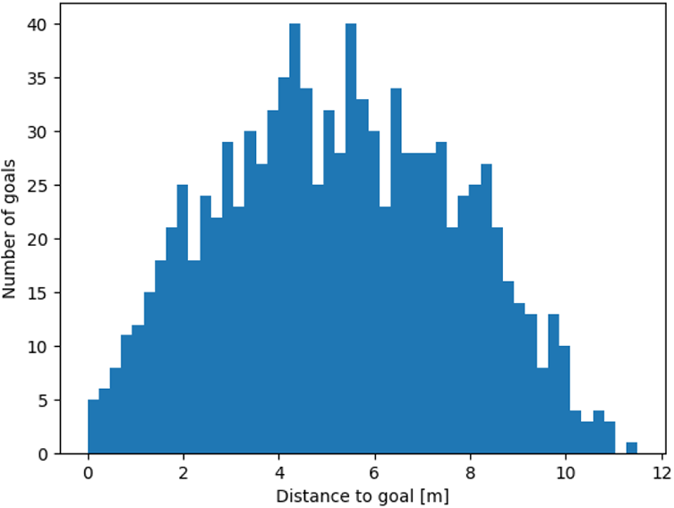
In this way, each evaluated navigation system was tasked with reaching 1000 goals in each of the three stages. As can be seen in the histogram in Figure 9, the distances between the goals range from $0.5 m$ to a little more than $10 m$ , while the average distance is about $5 m$ . The quantitative results of the evaluation are shown in Table 3.

Figure 9.

Distribution of the distances to a goal in the third experiment.

Table 3.

Evaluation of the navigation on 100 consecutive navigation tasks consisting of 10 goals each.^a

	Stage 1	Stage 2	Stage 3
Method	#	#	#
Ours	973	962	957
T.S.Dijkstra	941	727	598
T.S.D*Lite	937	743	625

^a The total number of successfully reached goals is represented for each method and each stage.

As can be seen in Table 3, the performance of the T.S. navigation methods, both with the Dijkstra planner and the D* lite planner, drops in stages 2 and 3, due to the degradation of the map. The results of the third experiment further confirm the results from the previous experiments. We inspected the failures of all three methods in the first stage, and the vast majority are due to goals which are too close to obstacles for a safe approach.

The results in all three experiment are consistent and conform with observations of the robots in our lab. Namely, map-based navigation methods can perform poorly if they are initialized with a map that does not conform with the real environment. As the experiments show, this is true even if the map is being updated and the path planner is replanning the trajectories using the updated map. In most cases, the initial inaccuracies cause the localization to fail, which causes the map repairing to fail. As stated in the Introduction, if significant map changes are expected to happen, and the environment does not contain any maze-like features, one possible solution is using a map-less approach.

LSTM policy on a real robot

In the end, to demonstrate that the LSTM policy is transferable to a real robot, we applied the learned policy on the TurtleBot robot depicted in Figure 4(a) and ran the robot in a laboratory environment which is depicted in Figure 10. The laboratory is a typical work environment containing a lot of unstructured obstacles of different scales, like chair and table legs, computers, small tables, cables, and so on. These types of obstacles were not observed by the robot during training.

Figure 10.

The executed trajectories in the environment.

The executed trajectories are visualized in Figure 10 along with a map of the environment. The robot was initialized at the location marked with 0 and was then sequentially navigated to six goal locations. The navigation policy used for this experiment was the same one used in the experiments in simulation and no additional preprocessing of the input was done.

The executed trajectories are qualitatively the same as the trajectories produced in simulation, predominantly due to the severe randomization of the environments during training. Our system was able to navigate to all of the given goals. The average speed of the robot in this experiment was $0.33 m/s$ . Comparing this to the average speed of $0.40 m/s$ across all experiments in simulation, we can see that the performance is comparable without performing any domain adaptation.

Conclusion

In robotic navigation scenarios where the map is rapidly changing, working with maps can be impractical or impossible. Additionally, in the map-based scenarios, the deployment of a mobile robot is delayed, since a map must be built beforehand. Furthermore, the environment should be adapted so that a reliable map can be built. To address these difficulties, in this work, we develop a map-less navigation approach.

We cast the mobile navigation task as an MDP. Our approach is based on a deep neural network trained with the A2C RL method. A large number of samples needed for training a deep neural network are generated in a simulated environment, without requiring manual labeling. We also show that such a policy is transferable to a real robot without any special domain adaptation. The main reasons for this are the regularization during training and the slight abstraction from the exact robot model in the generation of the actions.

The learned policies are applied on a robot equipped with a laser range scanner. We evaluate our approach against the ROS navigation stack and show that, as the environment deviates from the map, our method outperforms the standard approach.

In the future, we will expand our approach to work in environments with dynamic obstacles. For this purpose, we have built a simulator for pedestrians that uses a state of the art model for movement of human crowds. We plan to utilize the modeling power of LSTM networks to train a navigation policy which uses the past movements of the detected humans to make safe decisions on where the robot should move next.

Footnotes

Declaration of conflicting interests

The author(s) declared no potential conflicts of interest with respect to the research, authorship, and/or publication of this article.

Funding

The author(s) disclosed receipt of the following financial support for the research, authorship, and/or publication of this article: This work was supported in part by the Slovenian Research Agency (ARRS) project J2-9433 and program P2-0214.

ORCID iD

Matej Dobrevski

References

Dobrevski

Skocaj

. Map-less goal-driven navigation based on reinforcement learning. In: Computer Vision Winter Workshop, Czech Republic, February 5–7, 2018.

Puterman

. Markov decision processes: discrete stochastic dynamic programming. Hoboken: John Wiley & Sons, Inc., 1994.

Kaelbling

Littman

Cassandra

. Planning and acting in partially observable stochastic domains. Artif Intell 1998; 101: 99–134.

Mnih

Mirza

Graves

, et al. Asynchronous methods for deep reinforcement learning. In: The 33rd International Conference on Machine Learning (ICML 2016), New York City, 19–24 June 2016.

Watkins

CJCH

Dayan

. Q-learning. Mach Learn 1992; 8: 279–292.

Sutton

McAllester

Singh

, et al. Policy gradient methods for reinforcement learning with function approximation. In: NIPS 99, Cambridge, MA, USA, 1999, pp. 1057–1063.

Mnih

Kavukcuoglu

Silver

, et al. Human-level control through deep reinforcement learning. Nature 2015; 518: 529–533.

Wang

Schaul

Hessel

, et al. Dueling network architectures for deep reinforcement learning. In: International conference on machine learning. PMLR, New York, 19–24 June 2016, pp. 1995–2003.

van Hasselt

Guez

Silver

Deep reinforcement learning with double q-learning. In: AAAI, Phoenix, Arizona, USA, February 2016.

10.

Lin

. Self-improving reactive agents based on reinforcement learning, planning and teaching. Mach Learn 1992; 8: 293–321.

11.

Schaul

Quan

Antonoglou

, et al. Prioritized experience replay. In: 4th International Conference on Learning Representations, ICLR, San Juan, Puerto Rico, 2–4 May 2016.

12.

Schulman

Levine

Jordan

, et al. Trust region policy optimization. In: ICML, Lille, France, 2015.

13.

Schulman

Wolski

Dhariwal

, et al. Proximal policy optimization algorithms. ArXiv 2017; abs/1707.06347.

14.

Lillicrap

Hunt

Pritzel

, et al. Continuous control with deep reinforcement learning, 2015. In: 4th International Conference on Learning Representations, ICLR 2016, San Juan, Puerto Rico, 2–4 May 2016.

15.

Abdel

Jaradat

Al-rousan

, et al. Reinforcement based mobile robot navigation in dynamic environment. Robot Comput Integ Manuf 2011; 27: 135–149.

16.

Konar

Chakraborty

Singh

, et al. A deterministic improved q-learning for path planning of a mobile robot. IEEE Trans Syst Man Cybern Syst 2013; 45: 1141–1153.

17.

Das

Mandhata

Behera

, et al. An improved q-learning algorithm for path-planning of a mobile robot. Int J Comput Appl 2012; 51: 40–46.

18.

Wen

Chen

, et al. The Q-learning obstacle avoidance algorithm based on EKF-SLAM for NAO autonomous walking under unknown environments. Robot Autonom Syst 2015; 72: 29–36.

19.

Smith

Cheeseman

. On the representation and estimation of spatial uncertainly. IJRR 1986; 5: 56–68.

20.

Gupta

Davidson

Levine

, et al. Cognitive mapping and planning for visual navigation. In: CVPR, Honolulu, HI, USA, 21–26 July 2017.

21.

Sadeghi

Levine

. (CAD)² RL: real single-image flight without a single real image. arXiv:161104201 2016.

22.

Xie

Wang

Markham

, et al. Towards monocular vision based obstacle avoidance through deep reinforcement learning. In: RSS Workshop on New frontiers for deep learning in robotics, Boston, USA, 15 July 2017.

23.

Bruce

Sünderhauf

Mirowski

, et al. One-shot reinforcement learning for robot navigation with interactive replay. In: NIPS, workshop on acting and interacting in the real world, Long Beach, CA, USA, 4–9 December 2017.

24.

Mirowski

Pascanu

Viola

, et al. Learning to navigate in complex environments. In: 5th International Conference on Learning Representations, ICLR 2017, Toulon, France, 24–26 April 2017.

25.

Zhu

Mottaghi

Kolve

, et al. Target-driven visual navigation in indoor scenes using deep reinforcement learning. In: ICRA, Singapore, 29 May–3 June 2017.

26.

Kulhanek

Derner

de Bruin

, et al. Vision-based navigation using deep reinforcement learning. In: ECMR, Prague, Czech Republic, 4–6 September 2019.

27.

Leiva

Lobos-Tsunekawa

Ruiz-del Solar

Collision avoidance for indoor service robots through multimodal deep reinforcement learning. In: RoboCup, Cham: Springer, 2019. pp. 140–153.

28.

Tai

Paolo

Liu

Virtual-to-real deep reinforcement learning: continuous control of mobile robots for mapless navigation. In: IROS, Vancouver, BC, Canada, 24–28 September 2017.

29.

Sutton

Barto

. Reinforcement learning: an introduction. Cambridge, MA: The MIT Press, 2017.

30.

Dobrevski

Skočaj

. Deep reinforcement learning for goal-driven robot navigation. In: 5th International Conference on Learning Representations, ICLR 2017, Toulon, France, 24–26 April 2017.

31.

OpenAI. Learning dexterous in-hand manipulation. IJRR 2019; 39: 3–20.

32.

Tobin

Fong

Ray

, et al. Domain randomization for transferring deep neural networks from simulation to the real world. In: IROS, Vancouver, BC, Canada, 24–28 September 2017.

33.

Fox

. Adapting the sample size in particle filters through kld-sampling. IJRR 2003; 22: 985–1003.

34.

Fox

Burgard

Thrun

. The dynamic window approach to collision avoidance. IEEE Robot Autom Mag 1997; 4: 23–33.

35.

Koenig

Likhacev

. D* Lite. In: The Eighteenth National Conference on Artificial Intelligence, Alberta, Canada, 28 July–1 August 2002.

36.

Giorgio Grisetti

Burgard

. Improved techniques for grid mapping with rao-blackwellized particle filters. IEEE Trans Robot 2007; 23: 34–46.

Deep reinforcement learning for map-less goal-driven robot navigation

Abstract

Keywords

Introduction

Related work

Approach

Reinforcement learning

Optimization

A2C

Navigation as a (PO)MDP

Learning in simulation

Evaluation

FF policy on a real robot

LSTM policy in simulation

LSTM policy on a real robot

Conclusion

Footnotes

Declaration of conflicting interests

Funding

ORCID iD

References