Combining closed-form and numerical solutions for the inverse kinematics of six-degrees-of-freedom collaborative handling robot

Abstract

In the process of solving the inverse kinematics of six-degrees-of-freedom collaborative robots, the numerical solution has problems such as low accuracy and singular configurations. Moreover, due to the high coupling of its position and attitude, the direct closed-form solution fails. To address these problems, an inverse kinematics algorithm that combines closed-form and numerical solutions was proposed. The Jacobian matrix was established based on the forward kinematics equation of the six-degrees-of-freedom collaborative robot. Its inverse matrix was obtained by a singular value decomposition of the matrix using the Manocha elimination method to avoid the singularities of the Jacobian matrix. The optimal inverse kinematics solution was obtained using the Newton–Raphson iterative method. A computer simulation implemented in MATLAB and Visual C++ was used to evaluate the accuracy and speed of the proposed algorithm. The results of the trajectory planning experiments demonstrate that the algorithm satisfies the requirements for real-time smooth motion. This study of inverse kinematics lays the theoretical foundation for solutions to the inverse problem and real-time control of collaborative robots.

Introduction

Because it is impossible to realize full automation in flexible production, man–machine collaboration is a feasible way to improve the productivity of semiautomated systems. ¹ Collaborative robots, which have the characteristics of high flexibility, simple programming and rapid configuration, have a wide range of potential applications in the service industry, such as health care, education and retail. ² In practical applications, the position and direction of the end effector are usually given or predetermined. Therefore, inverse kinematics plays a crucial role in solving the real-time control process and trajectory planning problems of robotic manipulators. ³ Furthermore, due to the inherent nature of the Non-deterministic Polynomial (NP) problem and complex nonlinear equations, computing the inverse kinematics solution of a multi-degree of freedom (DOF) serial robotic manipulator requires more computational resources and time compared to the forward kinematics. ⁴ There are two main methods for solving inverse kinematics: closed-form solutions and numerical solutions. ⁵ To improve flexibility, most collaborative robots adopt a design configuration that uses three parallel axes. There is no universal closed-form solution method for the inverse kinematics equation of this type of robot; therefore, many numerical solutions have been adopted. ⁶ However, numerical solutions have problems, such as low accuracy and complex solution processes. Because of the variable structure of the robot itself, the algorithm has different time and space requirements, and there are few algorithms that can satisfy these requirements. ⁷

In recent years, many researchers have made significant efforts to solve the inverse kinematics problem of six-degrees-of-freedom (6-DOF) robotic arm. Primrose was the first to demonstrate that the inverse solution of a 6 R robot with a general configuration has at most 16 sets of real roots. ⁸ Lee and Liang constructed 14 basic equations of inverse kinematics, used low-dimensional ideas to simplify the multivariate nonlinear equations into one-dimensional 16-degree equations, and finally obtained 16 exact solutions of inverse kinematics. The inversion process is very complicated. ^9,10 Xu et al. proposed an analytic algorithm for the kinematics inverse algorithm for the palletizing robotics. This algorithm has practicality to a certain extent, but it always has a problem that the attitude corresponds to multiple analytical results, and the unique solution cannot be determined. ¹¹ Wang et al. used a damped least-squares method to solve the inverse solution of a seven revolute-joint (7 R) 6-DOF robot by comparing the 7 R 6-DOF robot with the equivalent 6 R robot, but an approximate solution was not considered. ^12,13 Chu et al. proposed a Robotics kinematics inverse algorithm based on the reconfigurable method. Simultaneously, the simulation robotic arm was designed based on the algorithm. The practice shows that the robotic arm under the algorithm is very flexible, but the design process is too complicated. The number of iterations of the solution result is too many, so the actual algorithm is not efficient. ¹⁴ Hang and Savkin have proposed using competitive neural networks to solve the inverse kinematics problem of robotics using mechanical arm grabbing, but they are limited to specific robotics, and they are not implemented in the actual algorithm verification. ¹⁵ Amici and Cappellini obtained an inverse solution through the numerical inversion of a Jacobian matrix combined with a soft computing method, but its accuracy was low. ¹⁶ Yuan-Yuan and Wei proposed a simulated annealing algorithm and genetic algorithm that could calculate the inverse solution of a robot. This approach can achieve a certain accuracy but requires a large amount of calculation. ¹⁷ Zhi-jian and Jian-hua proposed a fast selection algorithm for analytical solutions based on the mathematical characteristics and motion continuity of the problem but did not consider singular problems. ¹⁸

Most of the above robot kinematics inverse solutions have convergence problems, and the iterative process is too complicated, which affects the efficiency and quality of the entire algorithm. ^19,20 At the same time, in the actual application of collaborative robots, because of factors such as special configurations or limitations of the approach, the traditional inverse solution is low in accuracy and prone to problems such as singular configurations. To solve these problems, an algorithm combining a closed-form solution with a numerical solution was proposed, and the inverse kinematics equation of a 6-DOF collaborative robot was constructed. To further reduce the computational complexity of joint quantization, this study introduces the Newton–Raphson iteration method to obtain optimal inverse kinematic solutions. To evaluate this approach, simulations and trajectory planning experiments were conducted, demonstrating its significant advantages compared to traditional inverse kinematics algorithms. The combined algorithm has faster solution and stability under higher precision and is not limited by the configuration of the manipulator; therefore, it can effectively solve the problem of inverse kinematics solution of the 6-DOF collaborative robot.

Forward kinematics analysis

A collaborative 6-DOF lightweight handling robot with a 3 kg load was designed. The structure of the robot was designed to be modular. Depending on the joints, the robot was divided into six modules, and the kinematic pair of each module was a rotary axis. The joints are divided into two categories, joints 1, 2, and 3, which are used for large motions and to determine the location of the claw, and smaller joints 4, 5, and 6 with mounting holes reserved at the end, which are utilized to determine the posture of the claw. A three-dimensional model of 6-DOF collaborative robot is shown in Figure 1.

Figure 1.

6-DOF collaborative robot.

The inverse kinematics solution of the robot is based on the forward kinematics solution, and the position and orientation of the end are obtained by the forward solution, which is used as the input to calculate the inverse solution. ²¹ According to the structural parameters and dimensions of the 6-DOF lightweight collaborative robot, the Denavit–Hartenberg (D-H) parameter method ²² was used to establish the six-axis space coordinate system of the robot. The D-H model of the robot is shown in Figure 2, and its parameters are listed in Table 1.

Figure 2.

D-H model.

Table 1.

Link parameters of 6-DOF collaborative robot.

Joint	Link length ai (mm)	Link twist αi (°)	Link offset di (mm)	Joint angle θi (°)	Range of joint rotation (°)
1	0	−90	0	θ 1 (0)	−90 to 90
2	a 2	0	0	θ 2 (−90)	−165 to −15
3	a 3	0	0	θ 3 (0)	−60 to 60
4	0	90	d 4	θ 4 (90)	30 to 150
5	0	−90	d 5	θ 5 (0)	−60 to 60
6	0	0	d 6	θ 6 (0)	−180 to 180

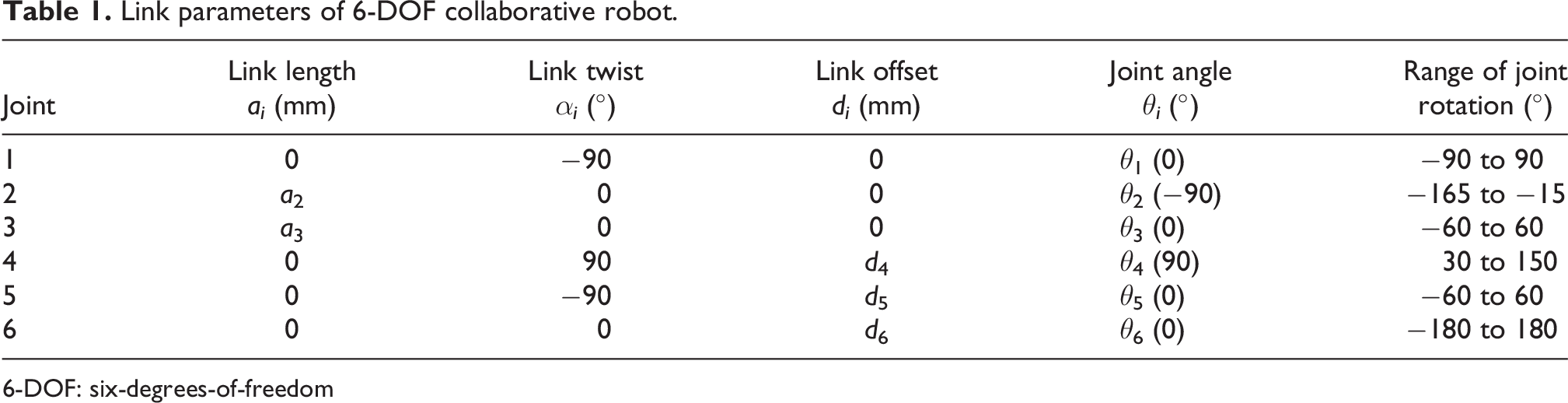
6-DOF: six-degrees-of-freedom

The transformation matrix A _i between two adjacent connecting rods is obtained according to the translation and rotation theory of the space coordinate system

$A_i=\left[\begin{array}{cc}\begin{array}{cc}c{\theta }_i& -s{\theta }_{i}c{\alpha }_i\\ s{\theta }_i& c{\theta }_{i}c{\alpha }_i\end{array}& \begin{array}{cc}s{\theta }_{i}s{\alpha }_i& a_{i}c{\theta }_i\\ -c{\theta }_{i}s{\alpha }_i& a_{i}s{\theta }_i\end{array}\\ \begin{array}{cc}0& s{\alpha }_i\\ 0& 0\end{array}& \begin{array}{cc}c{\alpha }_i& d_i\\ 0& 1\end{array}\end{array}\right]$

1

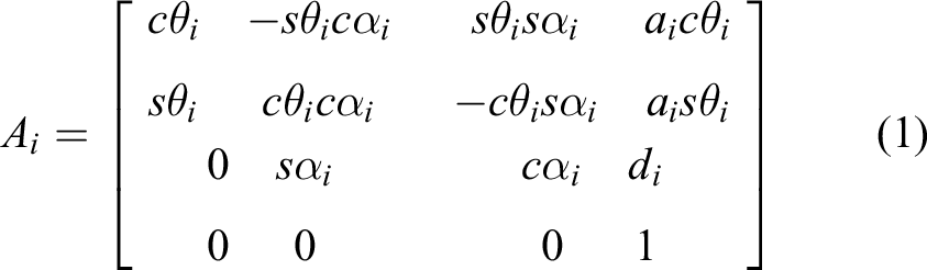
In equation (1), cθ_i = cosθ_i , sθ_i = sinθ_i , cα_i = cosα_i , and sα_i = sinα_i .

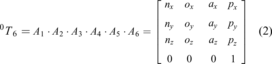
The 6-DOF lightweight collaborative robot is connected to a flange at the base to fix the gripper. Hence, the homogeneous pose transformation matrix of the end gripper relative to the base coordinate system is expressed as follows

${ }^0{T}_6=A_1\cdot A_2\cdot A_3\cdot A_4\cdot A_5\cdot A_6=\left[\begin{array}{cc}\begin{array}{cc}{n}_x& o_x\\ n_y& o_y\end{array}& \begin{array}{cc}{a}_x& p_x\\ a_y& p_y\end{array}\\ \begin{array}{cc}{n}_z& o_z\\ 0& 0\end{array}& \begin{array}{cc}{a}_z& p_z\\ 0& 1\end{array}\end{array}\right]$

2

Based on the differential transformation method and the differential mapping relation between the Cartesian space and joint space, the Jacobian matrix ${}_{ }{}^{T}J$ is obtained as follows

${ }^{T}J=\left[\begin{array}{cccccc}{j}_{11}& j_{12}& j_{13}& d_5{c}_5{c}_6& 0& 0\\ j_{21}& j_{22}& j_{23}& -d_5{c}_5{s}_6& 0& 0\\ j_{31}& j_{32}& j_{33}& -d_5{s}_5& 0& 0\\ { }^0{n}_z& c_6{s}_5& c_6{s}_5& c_6{s}_5& -s_6& 0\\ { }^0{o}_z& -s_6{s}_5& -s_6{s}_5& -s_6{s}_5& -c_6& 0\\ { }^0{a}_z& c_5& c_5& c_5& 0& 1\end{array}\right]$

3

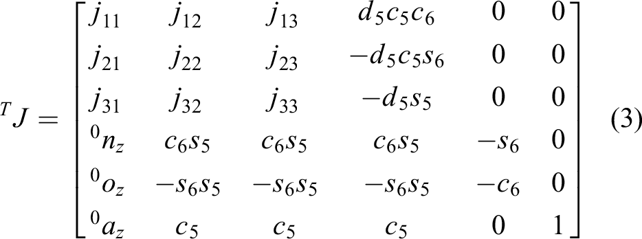
A singular configuration can be identified based on whether the determinant of the Jacobian matrix is zero. The determinant of the Jacobian matrix is

$|{ }^{T}J |=-s_5\left(de{t}_{44}-de{t}_{43}+de{t}_{42}\right)=\frac{s_5{a}_2{a}_3\left(d_5{c}_{q_2+2q_3+q_4}-d_5{c}_{2+4}-a_2{s}_{2+3}+a_3{s}_2+a_2{s}_{2-3}-a_3{s}_{q_2+2q_3}\right)}{2}$

4

Equation (4) reveals that a singular configuration of the robot has no relationship with joints 1 and 6. Given the configuration of the robot, it is clear that joints 1 and 6 do not cause a singular configuration during a practical grasping task. Because of the chain coupling structure of the robot, the determinant of the Jacobian matrix is very complicated. The singular configurations that occur when $|{}_{ }{}^{T}J|=0$ are as follows

$s_5=0,d_5\left(c_3-c_2{s}_3\right)=a_2{c}_2{s}_3$

${\theta }_3=0$

$c_4=0,2a_3{s}_3{c}_{2+5}=c_3(\left(d_5-a_2\right)c_2{s}_3+d_5{c}_3)$

${\theta }_5=0,\text{tan}{\theta }_3=\frac{d_5}{\left(a_2-d_5\right)\text{sin}\left(2{\theta }_3+{\theta }_2\right)}$

Inverse kinematics analysis

Inverse kinematics modelling

The inverse kinematics problem of a robot involves solving the angle of each joint of the robot when the position and orientation of the end-effector are given. Its solution enables the robot to realize kinematic simulation and trajectory planning. ²³ Because the inverse solution of the collaborative robot is difficult to obtain, the inverse kinematics model is analyzed using a combination of a closed-form solution and numerical solution. The Manocha elimination method was used to determine the forward kinematics, and the key matrix of the inverse kinematics was obtained using singular value decomposition (SVD) and the Newton–Raphson iteration method. The key matrix is converted into a numerical matrix with the link parameters.

First, according to the homogeneous transformation matrix, ${ }^0{T}_6$ is transformed to obtain

$Q\left(i,j\right)=A_3\cdot A_4\cdot A_5=A_2^{-1}\cdot A_1^{-1}\cdot T_{\text{end}}\cdot A_6^{-1}=R\left(i,j\right)$

5

In equation (5), Q(i, j) and R(i, j) represent the elements in row i and column j of matrices Q and R, respectively, where i and j = 1, 2,…, 4.

The elements Q(i, j) and R(i, j) are regarded as functions of the joint variable θ _i, namely,

$\left[\begin{array}{cccc}\left({\theta }_3,{\theta }_4,{\theta }_5\right)& \left({\theta }_3,{\theta }_4,{\theta }_5\right)& \left({\theta }_3,{\theta }_4,{\theta }_5\right)& \left({\theta }_3,{\theta }_4\right)\\ \left({\theta }_3,{\theta }_4,{\theta }_5\right)& \left({\theta }_3,{\theta }_4,{\theta }_5\right)& \left({\theta }_3,{\theta }_4,{\theta }_5\right)& \left({\theta }_3,{\theta }_4\right)\\ \left({\theta }_4,{\theta }_5\right)& \left({\theta }_4,{\theta }_5\right)& \left({\theta }_4,{\theta }_5\right)& \left({\theta }_4,{\theta }_5\right)\\ 0& 0& 0& 1\end{array}\right]=\left[\begin{array}{cc}\begin{array}{cc}\left({\theta }_1, {\theta }_2, {\theta }_6\right)& \left({\theta }_1, {\theta }_2, {\theta }_6\right)\\ \left({\theta }_1, {\theta }_2, {\theta }_6\right)& \left({\theta }_1, {\theta }_2, {\theta }_6\right)\end{array}& \begin{array}{cc}\left({\theta }_1,{\theta }_2\right)& \left({\theta }_1,{\theta }_2\right)\\ \left({\theta }_1,{\theta }_2\right)& \left({\theta }_1,{\theta }_2\right)\end{array}\\ \begin{array}{cc}\left({\theta }_1, {\theta }_2, {\theta }_6\right)& \left({\theta }_1, {\theta }_2, {\theta }_6\right)\\ 0& 0\end{array}& \begin{array}{cc}\left({\theta }_1,{\theta }_2\right)& \left({\theta }_1,{\theta }_2\right)\\ 0& 1\end{array}\end{array}\right]$

6

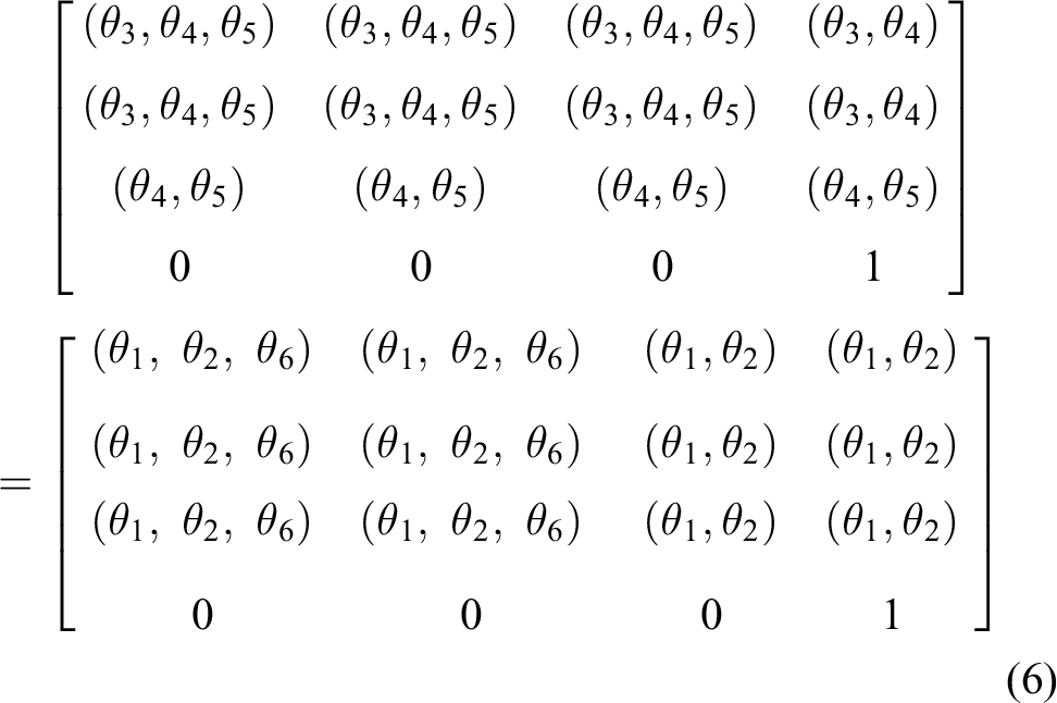
In equation (6), the elements in the third and fourth columns on both sides are independent with θ ₆, and the corresponding elements in the third column of matrices Q and R are equal. Both sides were obtained by multiplying by the orthogonal symmetric matrix and adding ${(\begin{array}{ccc}{a}_2& 0& d_2\end{array})}^T$

$\left(\begin{array}{ccc}{c}_2& s_2& 0\\ s_2& -c_2& 0\\ 0& 0& 1\end{array}\right)\stackrel{\sim }{h}=\left(\begin{array}{ccc}1& 0& 0\\ 0& -{\lambda }_2& {\mu }_2\\ 0& {\mu }_2& {\lambda }_2\end{array}\right)\left(\begin{array}{ccc}{c}_3& s_3& 0\\ s_3& -c_3& 0\\ 0& 0& 1\end{array}\right)\stackrel{\sim }{f}+\left(\begin{array}{c}{a}_2\\ 0\\ d_2\end{array}\right)$

7

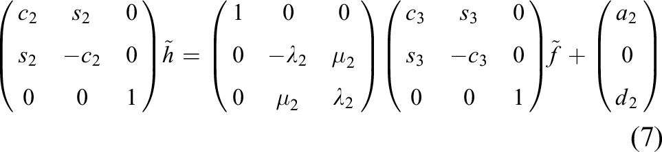
In equation (7), $\stackrel{\sim }{h}=\left(\begin{array}{c}{h}_1\\ h_2\\ h_3\end{array}\right),$ $\stackrel{\sim }{f}=\left(\begin{array}{c}{f}_1\\ f_2\\ f_3\end{array}\right)$ ; $h_v=FSC\left(c_1,s_1,c_2,s_2\right)$ ; $f_v=FSC\left(c_4,s_4,c_5,s_5\right)$ ; v = 1, 2, 3; and FSC(·) indicates that the function is a combination of the sines and cosines of their respective variables.

The corresponding elements in column 4 are equal and can be obtained in the same manner

$\left(\begin{array}{ccc}{c}_2& s_2& 0\\ s_2& -c_2& 0\\ 0& 0& 1\end{array}\right)\stackrel{\sim }{n}=\left(\begin{array}{ccc}1& 0& 0\\ 0& -{\lambda }_2& {\mu }_2\\ 0& {\mu }_2& {\lambda }_2\end{array}\right)\left(\begin{array}{ccc}{c}_3& s_3& 0\\ s_3& -c_3& 0\\ 0& 0& 1\end{array}\right)\stackrel{\sim }{\gamma }$

8

In equation (8), $\stackrel{\sim }{n}=\left(\begin{array}{c}{n}_1\\ n_2\\ n_3\end{array}\right)$ , $\stackrel{\sim }{\gamma }=\left(\begin{array}{c}{r}_1\\ r_2\\ r_3\end{array}\right)$ , $n_v=FSC\left(c_1,s_1,c_2,s_2\right)$ , $r_v=FSC\left(c_4,s_4,c_5,s_5\right)$ .

Vector P is used to represent matrix in equation (7), and vector L is used to represent matrix in equation (8). Fourteen linear independent equations are obtained from P, L, P·P, P·L, P×L, and (P·P)L−(2P·L)P, namely,

$\{\begin{array}{l}{P}_{L1}\left({\theta }_1,{\theta }_2\right)=P_{R1}\left({\theta }_3,{\theta }_4,{\theta }_5\right)\\ P_{L2}\left({\theta }_1,{\theta }_2\right)=P_{R2}\left({\theta }_3,{\theta }_4,{\theta }_5\right)\\ P_{L3}\left({\theta }_1\right)=P_{R3}\left({\theta }_3,{\theta }_4,{\theta }_5\right)\\ L_{L1}\left({\theta }_1,{\theta }_2\right)=L_{R1}\left({\theta }_3,{\theta }_4,{\theta }_5\right)\\ L_{L2}\left({\theta }_1,{\theta }_2\right)=L_{R2}\left({\theta }_3,{\theta }_4,{\theta }_5\right)\\ L_{L3}\left({\theta }_1\right)=L_{R3}\left({\theta }_3,{\theta }_4,{\theta }_5\right)\\ {\left(P·P\right)}_L\left({\theta }_1\right)={\left(P·P\right)}_R\left({\theta }_3,{\theta }_4,{\theta }_5\right)\\ {\left(P·L\right)}_L\left({\theta }_1\right)={\left(P·L\right)}_R\left({\theta }_3,{\theta }_4,{\theta }_5\right)\\ {\left(P\times L\right)}_{L1}\left({\theta }_1,{\theta }_2\right)={(P\times L)}_{R_1}\left({\theta }_3,{\theta }_4,{\theta }_5\right)\\ {\left(P\times L\right)}_{L2}\left({\theta }_1,{\theta }_2\right)={(P\times L)}_{R_2}\left({\theta }_3,{\theta }_4,{\theta }_5\right)\\ {\left(P\times L\right)}_{L3}\left({\theta }_1\right)={(P\times L)}_{R_3}\left({\theta }_3,{\theta }_4,{\theta }_5\right)\\ {\left[\left(P·P\right)L-\left(2P·L\right)P\right]}_{L1}\left({\theta }_1,{\theta }_2\right)={\left[\left(P·P\right)L-\left(2P·L\right)P\right]}_{R1}\left({\theta }_3,{\theta }_4,{\theta }_5\right)\\ {\left[\left(P·P\right)L-\left(2P·L\right)P\right]}_{L2}\left({\theta }_1,{\theta }_2\right)={\left[\left(P·P\right)L-\left(2P·L\right)P\right]}_{R2}\left({\theta }_3,{\theta }_4,{\theta }_5\right)\\ {\left[\left(P·P\right)L-\left(2P·L\right)P\right]}_{L3}\left({\theta }_1\right)={\left[\left(P·P\right)L-\left(2P·L\right)P\right]}_{R3}\left({\theta }_3,{\theta }_4,{\theta }_5\right)\end{array}$

9

The above 14 equations are simplified as follows

$\{\begin{array}{c}{L}_{6\times 2}^1{v}_0=R_{6\times 9}^1{v}_2\\ L_{8\times 6}^1{v}_1=R_{8\times 9}^1{v}_2\end{array}$

10

In equation (10), $L_{6\times 2}^1 \text{and} L_{8\times 6}^1$ are matrices with dimensions of 6 × 2 and 8 × 6, respectively, $R_{6\times 9}^1 \text{and }{R}_{8\times 9}^1$ are matrices with dimensions of 6 × 9 and 8 × 9, respectively, and their elements are functions containing unknown variables s₃ and c ₃. The coefficients of these variables are used to express the link parameters during the solution.

Using the Manocha elimination method, we have $x_i=\text{tan}\left({\theta }_i/2\right)$ , i = 1,…, 6, from the half angle formula

$s_i=\frac{2x_i}{1+x_i^2}{c}_i=\frac{1-x_i^2}{1+x_i^2}$

11

Substituting this into equation (10), s ₃ and c ₃ of $R_{6\times 9}^1$ and $R_{8\times 9}^1$ are replaced by x ₃, and we then eliminate θ ₁ and θ ₂ using Gaussian elimination to obtain six equations containing only θ ₃, θ ₄, and θ ₅. In addition, the parameter pairs s ₄, c ₄ and s ₅, c ₅ are replaced by x ₄ and x ₅, respectively, and 12 sets of equations are obtained, which are written in matrix form as follows

$({\displaystyle \sum }_A{x}_3^2+{\displaystyle \sum }_B{x}_3+{\displaystyle \sum }_C) v=0$

12

In equation (12)

$v={\left[x_4^3{x}_5^2 x_4^3{x}_5 x_4^3 x_4^2{x}_5^2 x_4^2{x}_5 x_4^2 x_4{x}_5^2 x_4{x}_5 x_4 x_5^2 x_5 1\right]}^T$

13

${\displaystyle \sum }_A=\left[\begin{array}{cc}{A}^{\prime }& 0\\ 0& A^{\prime }\end{array}\right] {\displaystyle \sum }_B=\left[\begin{array}{cc}{B}^{\prime }& 0\\ 0& B^{\prime }\end{array}\right] {\displaystyle \sum }_C=\left[\begin{array}{cc}{C}^{\prime }& 0\\ 0& C^{\prime }\end{array}\right]$

14

Moreover, ${\displaystyle \sum }_A , {\displaystyle \sum }_B, \text{and} {\displaystyle \sum }_C$ are key matrices for solving the inverse kinematics of the robot. In the case that there are three axes parallel to each other, we adopt SVD and the Newton–Raphson iterative algorithm to obtain the inverse matrix of the key matrix ${\displaystyle \sum }_A$ .

Inverse kinematics solution based on closed solution and numerical solution

The inverse kinematics equation expressed in matrix form is used for the symbolic operation, and the specific steps are as follows:

Step 1. Matrix equations were constructed by the vectors P and L, and 14 groups of linear equations were obtained using simple matrix operations.

Step 2. The above equations were simplified by shifting the terms to $L_{6\times 2}^1$ , $L_{8\times 6}^1$ , $R_{6\times 9}^1$ , and $R_{8\times 9}^1$ . According to the half angle formula, s ₃ and c ₃ are replaced by x ₃.

Step 3. The coefficient matrices were obtained by splitting the matrices such that each element was a constant expression.

Step 4. When the parameters of each connecting rod of the robot are not zero, the matrix expression of PA₁ ∼PC₂ of the 6 R robot with general configuration can be obtained. For a robot with a special configuration, when solving the inverse kinematics equation, it only needs to perform a symbolic operation to calculate the constant expressions of the PA₁ ∼PC₂ matrices.

Step 5. Assign the given link parameters and terminal pose to each expression of PA₁ ∼PC₂ to obtain a numerical matrix.

Step 6. After a series of matrix simplifications such as Gaussian elimination method, the key matrices ${\text{Σ}}_A$ , ${\text{Σ}}_B$ , and ${\text{Σ}}_C$ of this configuration are finally obtained.

The solution process is illustrated in Figure 3. Considering that several link parameters of the cooperative robot are zero, many elements of the symbol matrix are zero. Using the known link parameters to eliminate the unknown parameters, the sign matrices for $L_{6\times 2}^1$ and $L_{8\times 6}^1$ are obtained.

Figure 3.

Solution flowchart.

Parameters x ₃, x ₄, and x ₅ can be solved after the key matrices are obtained using the closed-form and numerical methods. To avoid the effect of the cumulative error of floating-point calculations on the accuracy of the solution, the matrix decomposition method is adopted to ensure the accuracy of the solution. When ${\displaystyle \sum }_A$ is a nonsingular matrix, the square matrix constructed using the key matrix is as follows

$M=\left(\begin{array}{cc}0& I\\ -{\displaystyle \sum }_A{ }^{-1}{\displaystyle \sum }_C & -{\displaystyle \sum }_A{ }^{-1}{\displaystyle \sum }_B \end{array}\right)$

15

In equation (15), I and 0 represent the 12 ×12 identity and zero matrices, respectively.

The eigenvalue of M is the solution of x ₃, and the corresponding eigenvector V is expressed as follows

$V=\frac{\left[\begin{array}{c}v\\ x_{3}v\end{array}\right]}{\left[\begin{array}{c}v\\ x_{3}v\end{array}\right]}$

16

Parameters x ₃, x ₄, and x ₅ are solved using eigenvector V, and θ ₃, θ ₄, and θ ₅ are subsequently solved. Next, θ ₁ and θ ₂ are solved using the matrix eigenvalue decomposition method. Finally, the joint angle θ ₆ was obtained.

There is a sizable number of matrix operations during the calculation, and to meet the required accuracy, an eigenvector V with a larger absolute value is selected to solve θ ₄ and θ ₅ to reduce the influence of cumulative errors in the floating-point calculations. When $|x_3|\le 1$ , we select the first 12 rows of eigenvector V; otherwise, the last 12 rows of eigenvector V are selected, which increases the accuracy of the solution. Considering the uncertainty in the maximum absolute value of vector $\nu$ in equation (12), the calculation results for θ ₄ and θ ₅ are as follows

${\theta }_4=\{\begin{array}{c}\begin{array}{c}2a\text{tan}\left(V\left(1\right)/V\left(4\right)\right)\text{ max}|V\left(i\right)|=|V\left(1\right)|\\ 2a\text{tan}\left(V\left(3\right)/V\left(6\right)\right)\text{ max}|V\left(i\right)|=|V\left(3\right)|\end{array}\\ \begin{array}{c}2a\text{tan}\left(V\left(7\right)/V\left(10\right)\right)\text{ max}|V\left(i\right)|=|V\left(10\right)|\\ 2a\text{tan}\left(V\left(9\right)/V\left(12\right)\right)\text{ max}|V\left(i\right)|=|V\left(12\right)|\end{array}\end{array}$

17

${\theta }_5=\{\begin{array}{c}\begin{array}{c}2a\text{tan}\left(V\left(1\right)/V\left(2\right)\right)\text{ max}|V\left(i\right)|=|V\left(1\right)|\\ 2a\text{tan}\left(V\left(2\right)/V\left(3\right)\right)\text{ max}|V\left(i\right)|=|V\left(3\right)|\end{array}\\ \begin{array}{c}2a\text{tan}\left(V\left(10\right)/V\left(11\right)\right)\text{ max}|V\left(i\right)|=|V\left(10\right)|\\ 2a\text{tan}\left(V\left(11\right)/V\left(12\right)\right)\text{ max}|V\left(i\right)|=|V\left(12\right)|\end{array}\end{array}$

18

By choosing a larger eigenvector, the overall calculation process is guaranteed to be stable, and the cumulative errors in the calculation process can also be reduced.

Inverse kinematics verification

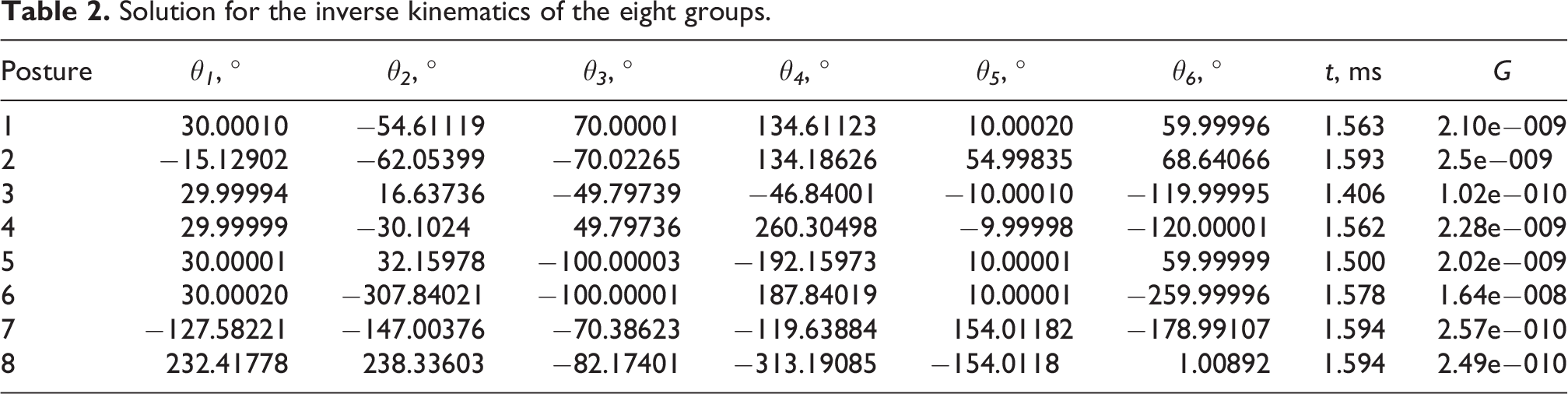
The effectiveness of the algorithm was verified on a computer configured with AMD Ryzen 7 5800 H with Radeon Graphics 3.20 GHz, 16.0 GB RAM and Windows 10 Professional operating system based on the parameters of each link of the robot and the pose matrix of the end point shown in equation (19). The abovementioned algorithms were implemented using Visual Studio 2019. Because there is no mathematical function library for matrix operations in C++, the MATLAB C++mathematical function library is called and the static link libraries are set in Visual C++. Thus, relevant functions can be called to calculate the matrix, thereby improving the efficiency of development. Combining the Newton–Raphson iterative algorithm, eight sets of inverse solutions for the robot were obtained, as shown in Table 2

${}_6{}^{0}T=\left[\begin{array}{cc}\begin{array}{cc}-0.85607& -0.22298\\ -0.39399& -0.30239\end{array}& \begin{array}{cc}-0.46629& 399.28178\\ 0.86795& 538.5436\end{array}\\ \begin{array}{cc}-0.33454& 0.92674\\ 0& 0\end{array}& \begin{array}{cc}0.17101& 129.85871\\ 0& 1\end{array}\end{array}\right].$

19

Table 2.

Solution for the inverse kinematics of the eight groups.

Posture	θ1 , °	θ2 , °	θ3 , °	θ4 , °	θ5 , °	θ6 , °	t, ms	G
1	30.00010	−54.61119	70.00001	134.61123	10.00020	59.99996	1.563	2.10e−009
2	−15.12902	−62.05399	−70.02265	134.18626	54.99835	68.64066	1.593	2.5e−009
3	29.99994	16.63736	−49.79739	−46.84001	−10.00010	−119.99995	1.406	1.02e−010
4	29.99999	−30.1024	49.79736	260.30498	−9.99998	−120.00001	1.562	2.28e−009
5	30.00001	32.15978	−100.00003	−192.15973	10.00001	59.99999	1.500	2.02e−009
6	30.00020	−307.84021	−100.00001	187.84019	10.00001	−259.99996	1.578	1.64e−008
7	−127.58221	−147.00376	−70.38623	−119.63884	154.01182	−178.99107	1.594	2.57e−010
8	232.41778	238.33603	−82.17401	−313.19085	−154.0118	1.00892	1.594	2.49e−010

In previous studies, some scholars used pose errors to establish fitness functions $J_{PP}$ to solve inverse kinematics solutions. ^24,25 In the robot inverse kinematics solution based on the improved fitness function combination method, Guang et al. proposed a fitness function $J_{DR}$ of an intelligent algorithm, combined with the analytical method to solve the inverse kinematics solution of the collaborative robot. The combined method and the original method were used to solve the problem, respectively, and the solution time is shown in Table 3. ²⁶

Table 3.

Inverse kinematics solution time for three methods.

Method	t, ms
$J_{PP}$	32
$J_{DR}$	4
Combine closed-form and numerical solutions	1.584

According to the data in Table 2, the inverse kinematics solution of the robot obtained using the elimination method is accurate to eight decimal places, which satisfies the positioning accuracy requirements of the robot.

The average solution time based on the improved fitness function combination method is 4 ms, and the average solution time of the original method is 32 ms. The hybrid programming approach of MATLAB and Visual C++ was used in this study, with an average computation time of 1.548 ms. The combination method exhibited a solution speed approximately 2.5 times faster than the method previously proposed in literature. When the inverse kinematics algorithm meets the accuracy requirements, the solution time is less than 4 ms, which meets the requirements for real-time inverse kinematics solution of the control system of the collaborative robot to realize grasping and sorting materials.

Experimental analysis of trajectory planning

The algorithm was employed in our 6 R-robot prototype to further verify the correctness and feasibility of the algorithm in the control of the robot moving along a predetermined trajectory. The experimental platform was set up as shown in Figure 4 and includes the robot body, control cabinet, laser tracker, target ball, and PC.

Figure 4.

Experimental platform for trajectory planning.

The arc track of the grasping workpiece was considered as an example. First, the trajectory curve of the task space was planned and discretized, the number of space interpolation points was set to 100, and three points in any space were selected, as listed in Table 4. Second, the robot was instructed to execute arc interpolation planning using the inverse kinematics algorithm. The trajectory curve of the robot’s gripper was determined using a laser tracker to record the sample points every 300 ms, and the obtained coordinate points were sent to MATLAB. The actual and theoretical trajectories are compared in Figure 5.

Table 4.

Arbitrary space coordinates of three points.

Coordinate points	X, m	Y, m	Z, m	Rz, rad	Ry, rad	Rz, rad
Starting point p 1	0.2093	0.3598	0.8145	1.3708	1.5708	0.7563
Intermediate point p 2	0.2045	0.3478	0.7836	1.3708	1.2708	0.3060
Ending point p 3	0.2058	0.3317	0.768	1.3708	1.0708	−0.6300

Figure 5.

Comparison of the actual and theoretical trajectories.

The actual trajectory had certain errors with respect to the theoretical trajectory. These errors were affected by the robot’s manufacturing accuracy, motion control accuracy, and how well the PID parameters are matched. Nevertheless, the maximum error is 2.459 mm, which meets the requirements of the robot’s trajectory planning in grasping-task scenarios.

Conclusion

In this study, an inverse kinematics algorithm that combines a closed-form solution and a numerical solution was proposed. The SVD based on the Manocha elimination method was used to solve the inverse matrix to avoid singularities in the Jacobian matrix. The Newton–Raphson iterative method was used to obtain the optimal solution of the inverse kinematics, which improved the accuracy of the solution.

The trajectory planning experiments showed that the resultant trajectory was smooth and the motion was stable during grasping tasks, which verifies that inverse kinematics modelling is reasonable and feasible. The algorithm has high solving accuracy, which can satisfy the requirements for smooth robot motion.

This study provides a theoretical basis for inverse kinematics solutions of series-coupled structure robots based on a combination of closed-form and numerical methods.