Sage Journals: Discover world-class research

Abstract

The increasing number of robots and the rising cost of electricity have spurred research into energy-reducing concepts in robotics. One such concept, elastic actuation, introduces compliant elements such as springs into the robot structure. This article presents a comparative analysis between two types of elastic actuation, namely, monoarticular parallel elastic actuation and biarticular parallel elastic actuation, and demonstrates an end-to-end pipeline for their optimization. Starting from the real-world system identification of an RRR robotic arm, we calibrate a simulation model in a general-purpose physics engine and employ in silico evolutionary optimization to co-optimize spring configurations and trajectories for a pick-and-place task. Finally, we successfully transfer the in silico optimized elastic elements and trajectory to the real-world prototype. Our results substantiate the ability of elastic actuation to reduce the actuators’ torque requirements heavily. In contrast to previous work, we highlight the superior performance of the biarticular variant over the monoarticular configuration. Furthermore, we show that a combination of both proves most effective. This work provides valuable insights into the torque-reducing use of elastic actuation and demonstrates an actuator-invariant in silico optimization methodology capable of bridging the sim2real gap.

Keywords

Actuation and joint mechanisms compliant joints and mechanisms evolutionary robotics methods and tools for robot system design optimization and optimal control

Introduction

With the ever-increasing number of robots and the increase in the cost of electricity, the energy-efficient design of robots is receiving increased attention.¹ Although some work minimizes the electrical energy consumption directly, others have focused on minimizing the actuator torque requirements.² The latter is a more general methodology for energy reduction, as it is independent of the actuator’s characteristics. Moreover, a decrease in torque requirements leads to a size and weight reduction of the actuator, which consequently leads to a cost reduction of the actuator and increases the safety.³ Indeed, it reduces the moving mass and increases the compactness of the robot.

Introducing elastic elements in the joints and robot structure, a concept often termed “Elastic Actuation” can help to reduce energy consumption⁴ and, more specifically, the torque requirements for actuators.⁵ There are several ways to implement elastic actuation. One way is to place the spring in parallel with the actuator with respect to the load. This approach, called parallel elastic actuation (PEA),⁶ can store and release energy without going through the actuator. This means that less energy is lost due to motor and transmission losses, which in turn results in higher energy efficiency and improves the system’s stability.^7
–9

Another potential energy-reducing concept, inspired by the musculature of humans and animals, is biarticular actuation (BA). “Biarticular” refers to the connection of two joints, which can be done by either an actuated or a passive component like a spring.^10,11 BA offers the possibility to transfer mechanical power between joints,¹² in particular from proximal toward distal joints,¹³ leading to an improvement in energy efficiency.¹⁴ For example, Oh et al.¹⁵ have shown that having biarticular muscles helps to increase the energy efficiency for human and animal motion.

As PEA and BA are not mutually exclusive, it is also possible to combine both in an attempt to exploit the benefits of each simultaneously. Chevallereau et al.¹⁶ have already combined both in a robotic leg, but only the placement of the actuators and the best actuation scheme have been optimized, and not the springs’ characteristics (stiffness, equilibrium angle, etc.). Cahill et al.¹⁷ and Morizono et al.¹⁸ have optimized the springs’ characteristics for a robotic leg and a robotic arm but not in terms of actuator torque requirements.

To the best of the authors’ knowledge, Bidgoly et al. were the first to investigate an optimal configuration of PEA and BA in terms of actuator torque requirements in a single robotic arm.¹⁹ Nevertheless, the torque profiles that can be generated by the PEA and BA implemented in their work can only be obtained using zero free-length springs. This requires incorporating a mechanism that allows the use of classical springs (with non-zero free-length) as zero free-length springs. Indeed, they did not consider the spring’s equilibrium position in the generated torque profile of the spring, while it is present and nonnegligible when classical springs are considered. Furthermore, all the results were obtained in simulation and were not verified with experiments on a real-world prototype. Marchal et al. addressed these limitations by implementing springs that produce a torque that depends on the equilibrium position and that can be more easily integrated into a robotic structure.¹ Moreover, they verified the simulation results by doing experiments on a real-world prototype built for this purpose. Their comparison was done on a pick-and-place task using a fixed trajectory that is shared among the different elastic actuation configurations. An ad hoc definition of a fixed trajectory can, however, induce unfairness in the comparison due to the trajectory unintentionally favoring a certain configuration.

Therefore, in our work, we provide a comparative analysis between monoarticular and biarticular elastic structures and a combination of both. We conduct this comparison using an RRR robotic arm (three revolute joints), and we target a pick-and-place task due to its simplicity and relevance in the industry. To provide a fair comparison between the benefits of the different forms of compliant configurations, we co-optimize the parameters of the spring configurations and trajectories.

As commonly done, one approach to do this is by defining a detailed mathematical model of the robot and its task.^1,19 However, the construction of such a model is a labor-intensive and highly problem-specific solution, as all robot and task-related physical phenomena have to be modeled exhaustively and precisely. A promising alternative is to use general-purpose physics simulators, as they do not require the manual definition of a problem-specific mathematical model.²⁰ General-purpose physics simulators allow rapid evaluations of arbitrary structures and tasks with ad hoc quality metrics.²¹ Consequently, they have served as the main backbone for many powerful robotic design optimization methodologies, such as the ones employed in evolutionary robotics.²² Their generality and speed, however, come with a fidelity trade-off, and often the acquired in silico evaluation results do not reflect the real-world counterpart as well as a problem-specific approach does.²³ This discrepancy can, however, be mitigated by (1) setting robot-related properties (e.g. link masses, link inertias) in the simulator according to conventional real-world system identification techniques and (2) introducing an explicit calibration step that automatically tunes the remaining unknown simulation parameters (e.g. unidentified task-related properties) to minimize the difference between real-world observations and the simulated counterpart.²⁴ Nevertheless, transferring in silico optimization results to the real world remains challenging. Demonstrative works in which this sim2real gap is overcome thus remain necessary on the path toward mitigating this fundamental issue.²⁵ Therefore, as the underlying backbone of our comparative analysis, we present a general in silico calibration and optimization pipeline based on evolutionary algorithms and explicitly showcase successful sim2real transfer of co-optimized designs and trajectories. An overview of our methodology is depicted in Figure 1.

Figure 1.

Overview of the end-to-end optimization pipeline for the elastic elements embedded within our RRR robotic arm. Two elastic configurations are implemented: PEA and BPEA. Starting from a real-world system identification (A), we calibrate a physics simulation model to provide rapid and realistic torque evaluations for a pick-and-place task (B). Using the in silico model, we co-optimize the elastic actuation configurations and trajectory using an evolutionary strategy named CMA-ES (C). Finally, we successfully transfer the co-optimized elastic elements and trajectory back onto the real-world prototype. PEA: parallel elastic actuation; BPEA: biarticular parallel elastic actuation; CMA-ES: covariance matrix adaptation evolution strategy.

To summarize, our contribution is twofold: (1) We provide insights into the influence of monoarticular and biarticular parallel elastic elements on actuator torque requirements, thereby providing an actuator invariant methodology for minimizing actuator torque requirements, and (2) we implement a general end-to-end robotic design optimization pipeline capable of successful sim2real transfer and showcase it on elastic elements and trajectory co-optimization. Our comparison between the different elastic actuation configurations is the first to include trajectory in the optimization. This increases fairness, as this mitigates the possibility of a fixed trajectory unfairly promoting certain configurations. Furthermore, our in silico calibration step is the first to extend to the successful sim2real transfer of both morphological (elastic elements) and controller (trajectory) parameters. By contrast, previous work focused solely on calibrating a fixed morphology to improve the sim2real transfer of the controller.²⁴ The novelty of our work thus lies in both these contributions individually and in their combination.

The remainder of this article is organized as follows: The second section describes the robot model, both of the considered elastic configurations and the link between the electrical energy consumption and the torque requirements. The third section defines the pick-and-place task that we target, the evolutionary optimization algorithm, our simulation calibration methodology, and the elastic elements and trajectory co-optimization. The fourth section discusses the validation of the calibrated in silico model and the co-optimization results. Finally, the fifth section concludes this study and discusses the limitations and future work.

Real-world system identification

Mathematical model

The type of robotic arm treated in this article is of RRR type (Figure 1). In this robotic arm, there are three electrical servo motors, each controlling a single joint. All the mechanical parameters are given in Table 1. They are found by using CAD software (Inventor) and validated experimentally, where stress analysis is performed to ensure that the prototype built with these parameters can handle a payload of 5 kg. Furthermore, limits of maximal angular velocities are chosen very close to the ones of the Kuka LBR iiwa 7 R800 to ensure safety, and maximal accelerations are imposed to ensure the smooth operation of the actuators. The equations of motion of the robot are given by²⁶

M (q) \ddot{q} + C (q, \dot{q}) \dot{q} + G (q) = τ_{1},

where $M (q)$ is the mass matrix (also called inertia matrix), $q$ are the joint displacements, $C (q, \dot{q})$ is the matrix of Coriolis and centrifugal forces, $G (q)$ is the gravitational torque vector and $τ_{l}$ is the load torque vector (also called the input torque seen by the actuator). Note that $M (q)$ , $C (q, \dot{q})$ and $G (q)$ can be derived from Table 1 using Lagrangian mechanics.

Table 1.

Mechanical parameters of the robot arm.^a

	Link 1	Link 2	Link 3
$m$ (kg)	$4.480$	$4.045$	$2.181$
$l$ (m)	$0.07$	$0.3$	$0.3$
$l_{c}$ (m)	$5.08 e - 2$	$8.06 e - 2$	$1.08 e - 1$
$I_{x x}$ (kg·m²)	$6.292 e - 2$	$1.440 e - 2$	$4.90 e - 3$
$I_{x y}$ (kg·m²)	0	$4.9 e - 4$	0
$I_{x z}$ (kg·m²)	$6.49 e - 3$	$9.67 e - 3$	$2.4 e - 4$
$I_{y y}$ (kg·m²)	$3.266 e - 2$	$6.831 e - 2$	$6.839 e - 2$
$I_{y z}$ (kg·m²)	0	0	0
$I_{z z}$ (kg·m²)	$6.292 e - 2$	$5.738 e - 2$	$6.460 e - 2$
	Joint 1	Joint 2	Joint 3
${\dot{q}}_{max}$ (°/S)	$90$	$90$	$90$
${\ddot{q}}_{max}$ (°/S²)	$180$	$180$	$180$

^a $m$ is the mass, $l$ is the length, $l_{c}$ is the distance between the joint and the center of gravity of the corresponding link, $I_{i j}$ ( $i = x, y, z$ and $j = x, y, z$ ) are the inertia parameters with respect to the center of gravity of the corresponding link, ${\dot{q}}_{max}$ is the maximum speed allowed, and ${\ddot{q}}_{max}$ is the maximum acceleration allowed.

Parallel elastic actuation

PEA places a spring in parallel with the actuator of a specific joint (Figure 2). It is considered as a monoarticular type of elastic actuation since it produces a torque only on the joint on which the parallel spring is placed. When PEAs are added to a robot’s joints, its equations of motion can be written as

M (q) \ddot{q} + C (q, \dot{q}) \dot{q} + G (q) = τ_{1} + τ_{p},

Figure 2.

PEA: $τ_{m, i}$ , $τ_{1}$ , $τ_{p,i}$ are the motor, load, and PEA-induced torque, respectively, for joint i. A positive value of $q_{i} - q_{eq, i}$ corresponds to the compression of the corresponding parallel spring and therefore to the production of a torque. PEA: parallel elastic actuation.

where $_{p}$ is the torque produced by the PEAs present on each joint. Since only unidirectional spiral torsion springs are considered, $_{p}$ is given by

τ_{p, i} = {\begin{array}{l} - k_{p, i} (q_{i} - q_{eq, i}) & if q_{i} \geq q_{eq, i} \\ 0 & else \end{array},

where $k_{p, i}$ is the spring stiffness of the parallel springs, $q_{eq, i}$ is the equilibrium angle of the corresponding springs, and $i = 1, 2, 3$ represents joints 1, 2, and 3. The torque produced by the unidirectional spiral torsion spring is zero when $q_{i} < q_{eq, i}$ because the extremity of this spring is not in contact anymore with the shaft on which it is supposed to rest to produce torque. The optimization of PEA corresponds to optimizing two parameters, namely, the stiffness $k_{p, i}$ and the equilibrium angle $q_{eq, i}$ of the spring. Note that if the orientation of the unidirectional spiral torsion spring is inverted, meaning that it starts to compress when $q_{i} \leq q_{eq, i}$ , the condition of (3) becomes $q_{i} \leq q_{eq, i}$ . As a result, depending on the orientation of the spring, the direction of the torque that the parallel spring of the PEA unit can produce is not the same. Nevertheless, since the gravitational torque is the dominant term in (1) and is always oriented in the same direction, only the case where the torque produced by the parallel spring is countering the gravitational torque can be energy-efficient and is considered in the optimization.

Biarticular parallel elastic actuation

Biarticular actuation refers to the simultaneous actuation of two joints by only one actuator or a passive component like a spring. In this article, since there already is an actuator controlling each joint, no additional actuator will be considered so as to not obtain a redundant robotic arm. Instead, a spring is placed with a biarticular connection. As such, we create a PEA that spans not only one but two joints, which we will refer to as “Biarticular Parallel Elastic Actuation”. In our robot, BPEA is achieved through the use of a mechanism composed of a unidirectional spiral torsion spring, a LIROS D-Pro Dyneema cable, and four pulleys (Figure 3). Note that there are four different arrangements of BPEA which each lead to different torques produced at the corresponding joints. Those four arrangements can be obtained by changing the winding direction of the cable on the different pulleys. Nevertheless, only one arrangement can produce a torque on both joints that counteracts gravity. Therefore, only this arrangement is considered in this article. With BPEA, (1) becomes

M (q) \ddot{q} + C (q, \dot{q}) \dot{q} + G (q) = τ_{l} + τ_{b},

Figure 3.

Biarticular parallel elastic actuation.

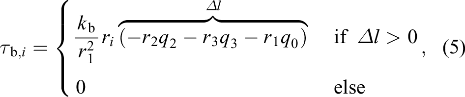
where $τ_{b}$ is the torque produced by the biarticular springs between joints 2 and 3, given by

τ_{b, i} = {\begin{array}{l} \frac{k_{b}}{r_{1}^{2}} r_{i} \overset{Δ l}{\overset{︷}{(- r_{2} q_{2} - r_{3} q_{3} - r_{1} q_{0})}} & if Δ l > 0 \\ 0 & else \end{array},

where r ₁, r ₂, and r ₃ are, respectively, the radii of the pulleys placed on link 1, joint 2, and joint 3, $k_{b}$ is the spring stiffness, $q_{0}$ is the equilibrium angle of the spring, and $i = 2, 3$ represents joints 2 and 3. The expression of $τ_{b, i}$ is found by solving the static equilibrium equations for links 2 and 3 as shown in Figures 6 and 7 in the Appendix. Therefore, when optimizing BPEA, there are five parameters to optimize, namely, $k_{b}$ , r ₁, r ₂, r ₃, and $q_{0}$ . Naturally, when PEA and BPEA are combined, (4) becomes

M (q) \ddot{q} + C (q, \dot{q}) \dot{q} + G (q) = τ_{l} + τ_{p} + τ_{b} .

Actuator energy consumption and torque requirements

We first explain the relation between (1) and the electrical energy consumption of the robotic arm actuators. A robot with three electrical servo actuators with harmonic drive transmission can be modeled as follows (when the effects of the inductance are neglected)

J_{m, i} {\ddot{q}}_{i} + ν_{i} {\dot{q}}_{i} = k_{t, i} I_{i} - τ_{f, i} ({\dot{q}}_{i}, τ_{l, i}),

U_{i} = R_{i} I_{i} + k_{t, i} {\dot{q}}_{i},

where $J_{m, i}$ are the inertias of the actuators, $ν_{i}$ are the actuators’ friction coefficients, $k_{t, i}$ are the motors’ torque constants, I_i are the motors’ currents, $τ_{f, i} ({\dot{q}}_{i}, τ_{l, i})$ are the torques due to the loads and the losses in the harmonic drives, U_i are the motors’ voltages, R_i are the electrical winding resistances of the motors, and $i = 1, 2, 3$ represent, respectively, joints 1, 2, and 3. Note that the term $k_{t, i} I_{i}$ is the actuator torque $τ_{a, i}$ . Regarding $τ_{f, i} ({\dot{q}}_{i}, τ_{l, i})$ , it is defined in the following way

τ_{f, i} ({\dot{q}}_{i}, τ_{l, i}) = c_{0, i} sgn ({\dot{q}}_{i}) + c_{l, i} τ_{l, i} + c_{v 2, i} sgn ({\dot{q}}_{i}) {\dot{q}}_{i}^{2} + c_{l 2, i} sgn ({\dot{q}}_{i}) τ_{l, i}

where $c_{0, i}$ , $c_{l, i}$ , $c_{v 2, i}$ , and $c_{l 2, i}$ are coefficients, and $sgn$ is the sign function. The determination of those coefficient values through a characterization of the actuators allows the computation of the load torque $τ_{l, i}$ without the need for any torque sensor on the robot. Indeed, knowing the velocity, the acceleration, and the current of the actuators, $τ_{l, i}$ can be computed as

τ_{l, i} = (\frac{1}{c_{l, i} + c_{l 2, i} sgn ({\dot{q}}_{i})}) (k_{t, i} I_{i} - J_{m, i} {\ddot{q}}_{i} - ν_{i} {\dot{q}}_{i} - c_{0, i} sgn ({\dot{q}}_{i}) - c_{v 2, i} sgn ({\dot{q}}_{i}) {\dot{q}}_{i}^{2})

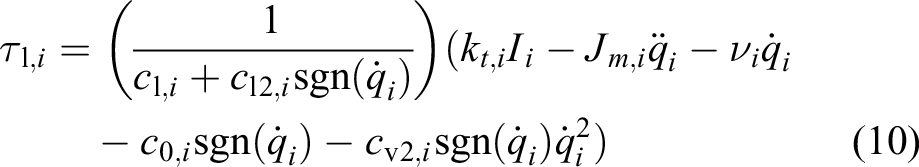
Note that (9) and (10) are specific to the actuators used in the real-world robot and are not necessarily correct for other types of actuators.

The electrical energy consumption of the actuators is given by the integral over the time of the product between the actuator current and voltage. By isolating the actuator current I_i in (7), and by taking into account that a pick-and-place task is considered, meaning that the term that includes the inertia is zero, one obtains

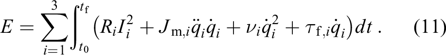
E = \sum_{i = 1}^{3} \int_{t_{0}}^{t_{f}} (R_{i} I_{i}^{2} + J_{m, i} {\ddot{q}}_{i} {\dot{q}}_{i} + ν_{i} {\dot{q}}_{i}^{2} + τ_{f, i} {\dot{q}}_{i}) d t .

Consequently, there are mainly three ways to reduce the electrical energy consumption of electrical actuators when the task the robot has to fulfill cannot be modified: (1) select an intrinsically efficient actuator, (2) the use of energy buffers, like elastic elements, and (3) trajectory optimization. Since the latter two approaches do not depend on the type of actuator used, they are more general and are the ones applied in this article. Indeed, by implementing elastic elements in the system, it is possible to reduce the first and last terms of (11) by storing and releasing gravitational energy, and therefore, the electrical energy consumption. The reduction of those two terms is explained by the fact that introducing elastic elements can help to reduce the load torque, and therefore I_i and $τ_{f, i} ({\dot{q}}_{i}, τ_{l, i})$ by looking at (7). On the other hand, by optimizing the trajectory, it is possible to decrease all the terms of (11) simultaneously by optimizing q_i , ${\dot{q}}_{i}$ , and ${\ddot{q}}_{i}$ . As we aim to minimize torque requirements in an actuator-invariant and general manner, we co-optimize the elastic actuation configurations with the trajectories. Consequently, our cost function becomes

E_{l} = \sum_{i = 1}^{3} \int_{t_{0}}^{t_{f}} τ_{l, i}^{2} (t) d t .

Indeed, if (11) is chosen as the cost function instead of (12), the optimal spring configurations and the trajectory would be different depending on the actuators used. Therefore, the optimization would lose its generality. Note that this cost function allows for the simultaneous reduction of the root mean square (RMS) and peak load torque. RMS load torque is closely related to the energy consumption of the actuator, and, usually, the sizing of the actuator, assuming that the peak load torque is only sustained for a small amount of time and does not dominate its sizing. Whereas peak load torque is more related to the sizing of the transmission device. Furthermore, both static and dynamic effects of the robot are taken into account in this cost function since $τ_{l, i}$ includes the gravitational torque, and the torques due to inertia, Coriolis, and centrifugal forces of the robot.

Task definition and in silico optimization

Pick-and-place task

In the manufacturing industry, robotic manipulators are commonly employed to move objects from one position to another. They often work in chains and repeatedly execute pick-and-place tasks, where speed and consistency are important features. To increase the industrial relevance of our results, we also consider a pick-and-place task in our work. Indeed, pick-and-place tasks cover a lot of applications (palletizing, bin picking, etc.) for which there is a payload close to the maximum load that the robot can handle, and where elastic actuation can help to decrease the actuators’ torque requirements.

Our pick-and-place task is composed of two phases: (1) The robotic arm moves from its initial position to a known release position by carrying a payload of 5 kg (called go phase), and (2) the robotic arm comes back to the initial position without the payload (called return phase). The initial/final position is $x_{0} = x_{f} = 0.15 m, y_{0} = y_{f} = 0 m, z_{0} = z_{f} = 0.07 m$ , and the release position is $x_{r} = 0.4 m, y_{r} = 0 m, z_{r} = 0.07 m$ as displayed in Figure 1. Note that the initial and release positions are chosen so that joints 2 and 3 move significantly during the task, while joint 1 is at a standstill. We made this choice because the load torque on this joint is negligible compared to joints 2 and 3. Indeed, gravity does not affect joint 1, and for this type of robot and task, the load torque is mainly due to gravity. Therefore, it is not interesting to implement springs on the first joint to reduce the actuator’s torque requirements, and making it move is useless ( $τ_{p,1} = 0$ and $τ_{b,1} = 0$ ). Consequently, only joints 2 and 3 are studied, and the cost function becomes

E_{l} = \sum_{i = 2}^{3} \int_{t_{0}}^{t_{f}} τ_{l, i}^{2} (t) d t .

For this type of robotic arm, there exist two joint configurations for which a single end-effector position is possible, namely, elbow-up and elbow-down configurations. Nevertheless, only the elbow-up configuration is considered here because it induces fewer collisions than the elbow-down configuration. As a result, one end-effector position corresponds to a single angular position of the joints.

The evolution strategy

To calibrate the in silico manipulator model and to subsequently optimize its trajectory and the design parameters of the springs, we use the covariance matrix adaptation evolution strategy (CMA-ES).²⁷ CMA-ES is a stochastic and derivative-free method for the numerical optimization of non-linear or non-convex continuous optimization problems. In general, evolution strategies mimic principles from biological evolution to optimize a distribution such that parameters sampled from that distribution optimize the objective function. In their canonical form, evolution strategies commonly use an n-dimensional isotropic Gaussian distribution, in which the distribution parameters only track the mean and standard deviation. CMA-ES extends upon this by tracking pairwise dependencies between samples and iteratively updating an additional distribution parameter: the covariance matrix. Intuitively, the covariance matrix allows CMA-ES to cast a wider net of samples when the best candidate solutions are far away or narrow the net when the best solutions are close together.

Based on preliminary trials, all experiments described below employ a population size of $64$ , random initial distribution means, and an initial standard deviation of $0.15$ .

A calibrated physics simulation model

Based on the real-world system identification, an in silico model of the manipulator was made in MuJoCo.²⁸ MuJoCo is a popular physics engine often used for robot simulation due to its high fidelity. To minimize the discrepancy between real-world and simulated results, parameters of the simulation that are unavailable in the real world are calibrated using the CMA-ES-based framework proposed by Urbain et al.²⁴ This framework tunes unknown parameters of the in silico model to minimize the difference between sensor data recorded during several trajectories on the real-world manipulator and the simulation model. Urbain et al. apply this framework to the calibration of a quadruped robot with a fixed morphology to improve the sim2real transfer of a locomotion controller trained in silico. We extend upon this and apply this framework to improve the sim2real transfer of both morphological (elastic elements) and controller (pick-and-place trajectory) parameters of a manipulator co-optimized in silico. In our case, valid sim2real transfer denotes a high similarity between simulated and real-world (load) torque evaluations. The inclusion of both morphological and controller parameters makes the calibration problem more complex, as this requires the calibrated in silico model to not only generalize beyond its original movement but also its original morphological configuration.

The parameters we adopt from the real-world system identification are link geometries (meshes), link masses, link inertias, actuator torque limits, and the P-controllers’ proportional gains. The calibrated MuJoCo parameters are joint friction loss (corresponds to a joint’s dry friction), joint damping (corresponds to a joint’s viscous friction), and joint armature (corresponds to a joint’s reflected inertia). We calibrate these parameters distinctly for each joint, as the joints do not have identical properties.

We collect a calibration data set on the real-world manipulator. This data set includes eight trajectories in total, each lasting $60$ s, and during which we record traversed joint positions q_i, velocities ${\dot{q}}_{i}$ , accelerations ${\ddot{q}}_{i}$ , and actuator torques $τ_{a, i}$ . The joints are actuated to follow a sinusoidal sweep with a varying amplitude trajectory, defined by the following equation for joint i

q_{i} = a_{i} \cdot \frac{t}{60} \cdot sin (2 π (f_{i}^{0} \cdot t + \frac{f_{i}^{1} - f_{i}^{0}}{2 \cdot 60} \cdot t^{2})) .

This definition allows us to vary the frequency (via $f_{i}^{0}$ and $f_{i}^{1}$ ) and amplitude (via a_i ) of the followed sinusoidal wave during the motion. In half of the trajectories, we increase this frequency over time ( $f_{i}^{0} < f_{i}^{1}$ ), while in the other half, we decrease it over time ( $f_{i}^{0} > f_{i}^{1}$ ). This change in frequency causes our calibration data set to contain both fast-to-slow and slow-to-fast trajectories. The amplitude always increases over time up to the given target a_i , which we set to the maximum allowed range of motion for each joint during pick-and-place. We further diversify this data set by adding or omitting the pick-and-place payload, and adding or omitting the PEA springs (with $k_{p,2} = 13.705 \frac{Nm}{rad}$ , $q_{eq,2} = 10$ , $k_{p,3} = 1.318 \frac{Nm}{rad}$ , and $q_{eq,3} = 140$ ). We do not include the BPEA configuration in our calibration data set to be able to validate the morphological generalization of our calibration.

Given this data set, we then calibrate our in silico model of the manipulator by minimizing the normalized root mean squared error (NRMSE) between recorded load torques $τ_{l}$ during the simulated and the real-world trajectories. We calculate $τ_{l}$ using (10) and normalize the root mean squared error using the standard deviation of the recorded real-world load torques.²⁹ We choose to minimize the error between recorded load torques as this encapsulates joint velocity, joint acceleration, and actuator torque. Furthermore, as described in the “Actuator energy consumption and torque requirements” section, our load torque formula incorporates a real-world characterization of the employed actuators. While we are unable to directly set the in silico counterpart of these actuator properties in the in silico model (MuJoCo does not parameterize these properties), we hypothesize that minimizing the difference in recorded load torques stimulates our calibration to mimic these actuator-related influences by tuning the joint properties. In essence, we thus shift the responsibility of mimicking these actuator influences to the joints. In addition, load torque is the minimization objective in the later elastic elements and trajectory co-optimization experiments. Consequently, we want to put extra focus on the realism of these load torque evaluations.

To avoid calibrating the simulation model to imitate noisy real-world data, we smoothen the recorded real-world signals using a Savitzky–Golay filter before calculating the NRMSE.³⁰ Furthermore, we drop the first and last 0.1s of data to avoid edge case instabilities. The resulting fitness of a candidate solution passed to the CMA-ES optimizer is then the load torque NRMSE summed over the joints and the eight trajectories.

The results and validation of this calibration are further detailed in the Results and discussion section.

Elastic element and trajectory co-optimization

Given the different types of elastic configurations, we have four distinct optimization scenarios: (1) stiff actuation (SA), (2) monoarticular parallel elastic actuation (PEA), (3) biarticular parallel elastic actuation (BPEA), and (4) the combination of monoarticular and biarticular parallel elastic actuation (PEA + BPEA). In all optimizations, the elastic configuration is co-optimized with the trajectory to minimize (13) using CMA-ES. Next to being beneficial for minimizing torque requirements, the inclusion of trajectory optimization makes the comparison between elastic configurations fairer.

The SA scenario does not employ elastic elements and mainly serves as a baseline for comparison. Consequently, in SA, we only optimize the trajectory. In the PEA scenario, the elastic parameters include the stiffness $k_{p, i}$ and equilibrium angle $q_{eq, i}$ of the parallel springs in both the second and third joints. In the BPEA scenario, the elastic parameters are the spring stiffness $k_{b}$ , the joint radii $r_{1..3}$ , and the initial angle of pretension of the spring $q_{0}$ . Finally, in the PEA + BPEA scenario, the elastic parameters include all of the above.

The trajectory is represented in joint space and is divided into separate go-phase and return-phase trajectories. This allows specialization within each phase and is beneficial due to the different characteristics these phases have as the payload is only attached in the go phase. The trajectories are defined by fixed start and stop positions (as discussed in the “Pick-and-place task” section), and five intermediate points per phase, $q_{1..5}^{go}$ and $q_{1..5}^{return}$ , to be optimized distinctly for both joints 2 and 3. These points are then interpolated over time using an Akima spline to form the complete trajectory.³¹ The duration of both these phases, $t_{go}$ and $t_{return}$ , is parameterized as well (bounded between 1s and 5 s) to include trajectory traversal speed in the optimization. This makes the trajectory parametrization more expressive and again allows the optimizer to specialize based on payload attachment.

Due to the continuous nature of CMA-ES optimization and the limited hardware availability, not all optimal parameter values can be perfectly replicated on the real-world prototype. These parameters are the spring stiffness values ( $k_{p, i}$ and $k_{b}$ ) and the BPEA joint radii ( $r_{1..3}$ ). Thus to evaluate the optimized parameters on the real-world prototype, we approximated these parameters by taking their closest available real-world equivalent. Not all parameters can, however, be equally closely approximated. To mitigate this issue and to maintain fairness between the real-world validation of the different configurations, we re-optimized the other parameters (spring pretension angles $q_{eq, i}$ and $q_{0}$ , and joint trajectories), while keeping the approximated ones fixed. Accordingly, the real-world prototype does not perfectly reflect the parameters found in the complete optimization. Nevertheless, as discussed further below, this discrepancy is negligible, and the same performance trends as in the simulator are observed in the real world.

In total, we thus conducted seven co-optimization experiments: the four original configurations and the three counterparts of the PEA, BPEA, and PEA + BPEA configurations wherein a subset of the parameters were fixed to viable real-world values.

Given the stochasticity of CMA-ES, all seven co-optimization experiments were run for $10$ independent trials. Based on preliminary convergence tests, every trial was given a strict $1000$ -generations cut-off. Given the population size of $64$ , this is equal to a total of 64,000 evaluations per trial. We substantiate our conclusions by applying statistical significance tests on the data obtained across all of these in silico trials. As we cannot assume the normality of recorded values, p-values are obtained with the Mann–Whitney rank-sum test. $p < 0.05$ was chosen as the threshold for statistical significance.

Results and discussion

Code for reproduction and videos of the simulated and real-world pick-and-place trajectories can be found on the project webpage (https://sites.google.com/view/elastic-actuation).

Validation of the in silico model calibration

A quantitative validation of the calibration is provided in Table 2. This table provides the NRMSE (defined in the “A calibrated physics simulation model” section) between recorded simulation and real-world joint angles $q$ , joint velocities $\dot{q}$ , joint accelerations $\ddot{q}$ , actuator torques $τ_{a}$ , and joint load torques $τ_{l}$ . An NRMSE value of zero corresponds to a perfect fit of the simulation signal on the real-world signal. An NRMSE value larger than one means that the average difference between both signals is higher than the standard deviation of the real-world signal, given that we normalize using this standard deviation. More intuitively, a constant simulation signal with a value equal to the average of the real-world signal would correspond to an NRMSE value of one. A simulated signal with an NRMSE lower or higher than one thus corresponds to, respectively, a better or worse fit than such a constant signal. The low load torque NRMSEs (the maximum is $0.4470$ ) show that the calibration gives the in silico model a good fit on the calibration data set.

Table 2.

NRMSE between recorded simulation and real-world values after calibration, averaged over joints and trajectories.^a

	Calibration data (train)					Co-optimization data (test)
	$q$	$\dot{q}$	$\ddot{q}$	$τ_{a}$	$τ_{l}$	$q$	$\dot{q}$	$\ddot{q}$	$τ_{a}$	$τ_{l}$
SA	0.0900	0.0806	0.1058	0.1764	0.4470	0.0552	0.3872	0.4470	1.2748	2.0031
PEA	0.0704	0.0776	0.1038	0.1662	0.3750	0.0068	0.0950	0.5871	0.2871	0.7401
BPEA	/	/	/	/	/	0.0036	0.0923	0.6355	0.3030	0.9002
PEA + BPEA	/	/	/	/	/	0.0046	0.0999	0.6645	0.2528	0.8521

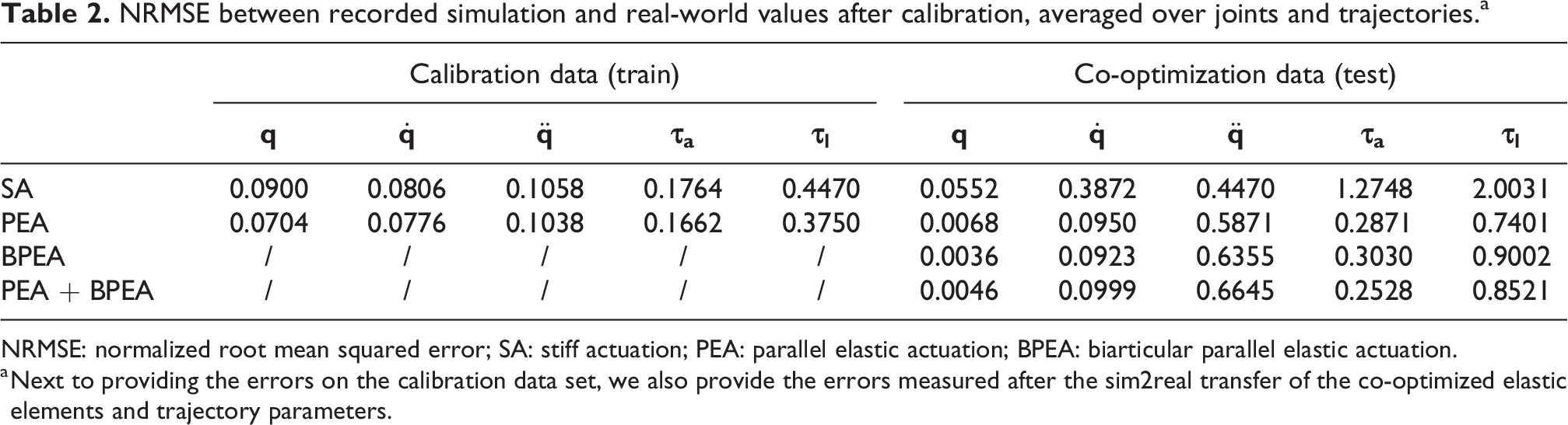
NRMSE: normalized root mean squared error; SA: stiff actuation; PEA: parallel elastic actuation; BPEA: biarticular parallel elastic actuation.

^a Next to providing the errors on the calibration data set, we also provide the errors measured after the sim2real transfer of the co-optimized elastic elements and trajectory parameters.

Table 2 also reports the recorded NRMSEs after the sim2real transfer of the co-optimized elastic elements and trajectory parameters. This comparison allows us to validate the generalization ability of the calibrated model to different elastic actuation configurations and trajectories, not included in the calibration data set. The results show an overall increase in load torque NRMSE for all configurations (the minimum is $0.7401$ ) compared to the NRMSEs recorded on the calibration data set. Nevertheless, the load torque NRMSEs of the PEA, BPEA, and PEA + BPEA configurations are below one, indicating a suitable fit. The load torque NRMSE of the SA configuration is, however, equal to $2.0031$ , indicating a poor fit.

A qualitative validation of the sim2real transfer of the co-optimized elastic elements and trajectory parameters is given in Figure 5. This figure shows the recorded simulation and real-world load torques of all configurations over trajectory time. For the BPEA (Figure 5(c)) and PEA + BPEA (Figure 5(d)) configurations, we can indeed see an appropriate fit. The simulated counterpart mainly provides a smoother version of the locally oscillating real-world load torques. Concerning the SA (cf. Figure 5(a)) and PEA (cf. Figure 5(b)) configurations, we can see that, although the simulated load torques follow a similar trend as the real-world load torques, there exists a slight offset between them. The PEA load torque NRMSE does not reflect this discrepancy due to the high standard deviation in its real-world load torque (we use standard deviation to normalize the RMSE).

Figure 4.

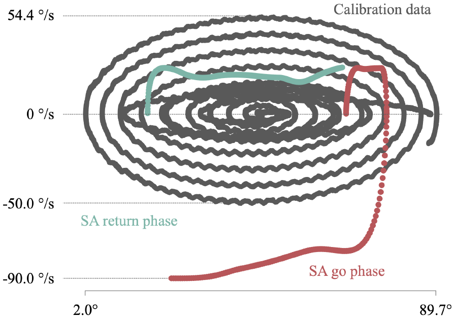
Scatterplot of the encountered joint position and joint velocity combinations of the second joint $(q_{2}, {\dot{q}}_{2})$ in the calibration data and in the optimized pick-and-place trajectory for the SA configuration. This demonstrates the discrepancy between traversed joint velocities during the go phase of the SA configuration’s pick-and-place trajectory and the joint velocities covered by the calibration data set.

Figure 5.

Evolution of the total load torque and (except for the stiff baseline) torque provided by the elastic elements during the pick-and-place trajectory. Total (load) torque is defined as the sum of the (load) torque on joints 2 and 3. Similarly as done in the calibration, here we also apply the Savitzky–Golay filter to smoothen the signals and we drop the first and last 0.1 s of each phase to avoid edge case outliers. This explains the discontinuities between the signals of the go and return phases.

The offset in load torque mainly originates from an underlying offset in actuator torque. This indicates that the tuned in silico friction properties do not perfectly mimic their real-world equivalent. A perfect match is, however, hard to attain since our in silico model does not explicitly include the effects of actuator frictions, load-dependent joint frictions caused by radial loads on the bearings, and harmonic drive frictions. Instead, our calibration step tries to imitate these effects by tuning the joint frictions, damping, and armatures using a cost function that is reliant on real-world system identification of these missing effects. While this succeeds for part of the trajectory space, as demonstrated by the lack of such a torque offset in the sim2real transfer of calibration trajectories and the BPEA and PEA + BPEA pick-and-place trajectories, other parts of the trajectory space exhibit a higher discrepancy. This discrepancy is highest for the go phase of the SA configuration because its optimized trajectory induces much higher joint velocities than the ones encountered in the calibration trajectories. Figure 4 demonstrates this.

Although our calibrated in silico model thus manages to generalize to unseen elastic actuation configurations, this shows that the generalization ability of our calibration is limited in the trajectory space. Consequently, there may exist a better real-world trajectory (for the SA and PEA configurations); one that the in silico co-optimization did not converge to due to the in silico load torque evaluations being slightly off in part of the trajectory space. Nevertheless, we do not require a true global optimum for each trajectory, as our focus lies on a comparative analysis between the different elastic actuation configurations. In this comparative analysis, our main interest lies in the ranking of their ability to reduce torque requirements and in the analysis of their torque behavior. This ranking remains valid, as (1) the same ranking persists when transferring the in silico co-optimization results to the real-world manipulator (as discussed further below and shown in Table 3), and (2) the simulator undershoots the amount of load torque required in these less accurate cases, thereby reducing the risk of these inaccuracies unfairly promoting the SA and PEA configurations and changing the rank. The analysis of the torque behavior of these elastic actuation configurations also remains valid, as the simulated load torque follows the same trends as the real-world load torque. We mainly include trajectory in the elastic elements optimization to avoid unintentionally favoring a certain elastic configuration due to the ad hoc definition of a fixed trajectory that is shared among these configurations. Although this makes the calibration more complex, we can thus conclude that this calibration is sufficient for our aims and that our sim2real transfer is successful.

Table 3.

Relative decrease in load torque requirements for every configuration, with respect to the stiff baseline (SA).^a

		Cost $E_{1}$		RMS load torque		Peak load torque
		Simulation	Real world	Simulation	Real world	Simulation	Real world
*Joint 2	PEA	66%	/	60%	/	32%	/
	PEA*	66%	62%	60%	58%	37%	6%
	BPEA	87%	/	76%	/	37%	/
	BPEA*	89%	93%	78%	82%	40%	33%
	PEA + BPEA	91%	/	81%	/	52%	/
	PEA + BPEA*	92%	94%	80%	83%	49%	41%
*Joint 3	PEA	77%	/	67%	/	40%	/
	PEA*	77%	70%	67%	63%	41%	42%
	BPEA	96%	/	87%	/	75%	/
	BPEA*	95%	93%	85%	83%	75%	73%
	PEA + BPEA	98%	/	91%	/	78%	/
	PEA + BPEA*	95%	95%	85%	85%	74%	66%

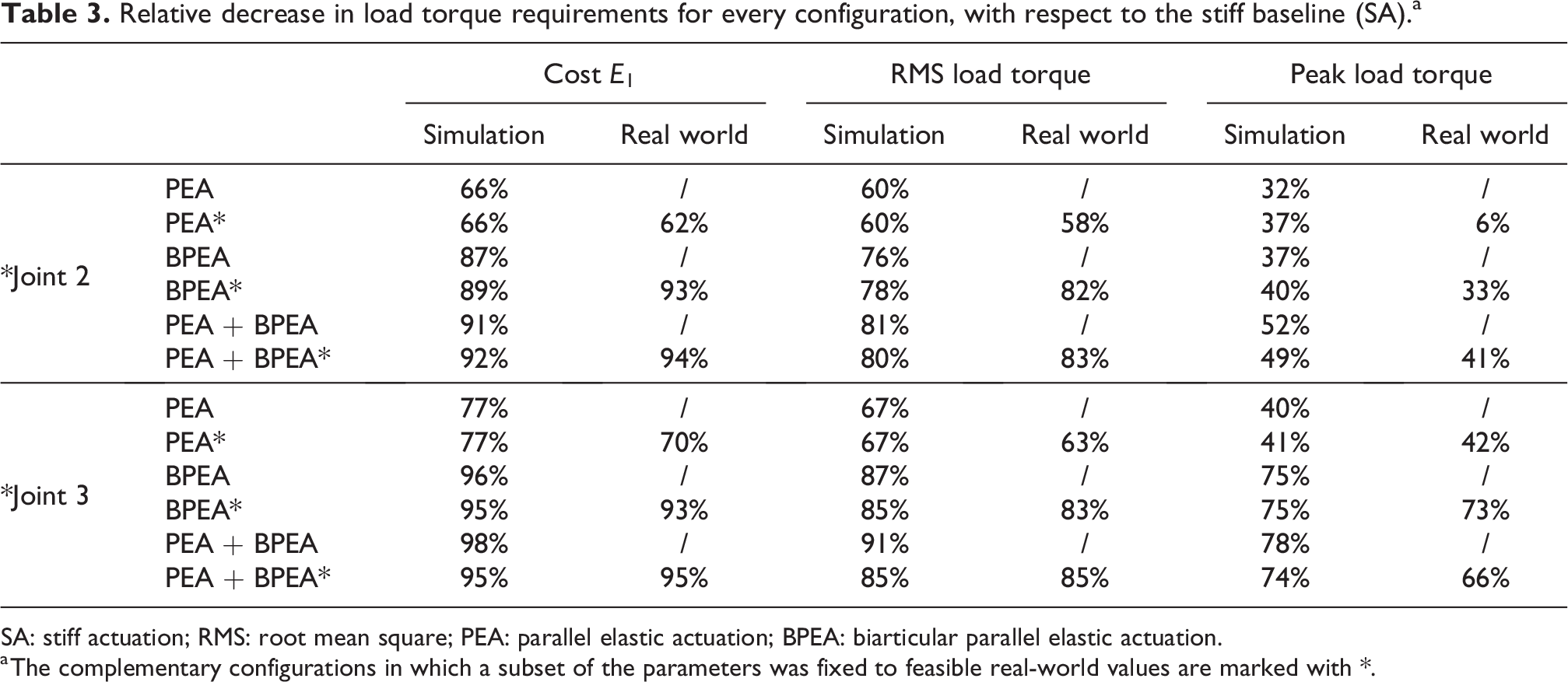
SA: stiff actuation; RMS: root mean square; PEA: parallel elastic actuation; BPEA: biarticular parallel elastic actuation.

^a The complementary configurations in which a subset of the parameters was fixed to feasible real-world values are marked with *.

Comparison of the elastic actuation configurations

Table 4 provides the best parameters found across all trials for each configuration. The resulting simulated and real-world cost, the RMS load torque, and the peak load torque (cf. (13)) are shown in Table 3. We present these values as relative decreases with respect to the values recorded with the SA baseline. These relative decreases demonstrate that implementing elastic elements in the robot structure heavily reduces the torque requirements of both joint’s actuators.

Table 4.

Optimal parameter values found for every spring configuration.^a

	PEA				BPEA					Trajectory
	joint 2		joint 3		$k_{b}$ (Nm/rad)	$q_{0}$ (°)	r ₁ (mm)	r ₂ (mm)	r ₃ (mm)	$t_{go}$ (s)	$t_{return}$ (s)
	$k_{p,2}$ (Nm/rad)	$q_{eq,2}$ (°)	$k_{p,3}$ (Nm/rad)	$q_{eq,3}$ (°)	$k_{b}$ (Nm/rad)	$q_{0}$ (°)	r ₁ (mm)	r ₂ (mm)	r ₃ (mm)	$t_{go}$ (s)	$t_{return}$ (s)
SA	/	/	/	/	/	/	/	/	/	1.2380	2.2960
PEA	13.7039	117.8275	0.6979	134.6711	/	/	/	/	/	3.3980	4.1260
PEA*	13.7052	119.0402	0.8755	111.4945	/	/	/	/	/	3.4400	4.1320
BPEA	/	/	/	/	9.9179	−71.4740	14.1	35.9	14.0	4.4897	3.5141
BPEA*	/	/	/	/	10.9664	−66.5492	15.0	36.0	14.0	4.1480	3.7780
PEA + BPEA	8.3133	101.5964	0.3873	134.4276	13.6963	−12.3297	14.0	36.0	18.6	3.7039	4.7141
PEA + BPEA*	8.2276	107.7522	0.6589	62.4224	13.7052	−8.5629	14.0	36.0	19.0	3.5000	4.1740

SA: stiff actuation; PEA: parallel elastic actuation; BPEA: biarticular parallel elastic actuation.

^a The complementary configurations, in which a subset of the parameters ( $k_{p,2}$ , $k_{p,3}$ , $k_{b}$ , and $r_{1..3}$ ) was fixed to feasible real-world values, are marked with *. $t_{go}$ and $t_{return}$ correspond, respectively, to the duration time of the go and return phases.

When evaluated in the physics simulator, the fully optimized PEA configuration reduces the total load torque cost (cf. (13)) of the SA baseline by 73% (66% and 77% for the second and third joints, respectively). The fully optimized BPEA configuration further improved upon this by reducing the total cost by 93% (87% and 96% for the second and third joints, respectively). As to be expected, the PEA + BPEA configuration reflects the best of both worlds and further improves upon both individual configurations by reducing the baseline’s total load torque cost by 95% (91% and 98% for the second and third joints, respectively). Taking into account all 10 in silico optimization trials, we can conclude that in this scenario (1) PEA, BPEA, and PEA + BPEA significantly outperform the SA baseline ( $p = 0.000091 < 0.05$ ), (2) BPEA significantly outperforms PEA ( $p = 0.000091 < 0.05$ ), and (3) PEA + BPEA significantly outperforms BPEA ( $p = 0.012874 < 0.05$ ). Given these results, it can be seen that the BPEA configuration serves as the main contributor to the PEA + BPEA configuration’s performance.

The complementary configurations (marked with an asterisk in Table 3), in which part of the parameters are fixed by real-world approximations, express similar statistically significant in silico results. As they show similar performance as in the complete optimizations, we can conclude that the approximated parameters to be used on the real-world prototype satisfyingly reflect the optimum found in the complete optimizations. In the case of the BPEA configuration, the approximated parameters even provided superior performance. This shows that the evolutionary optimizer does not guarantee a global optimum even when given multiple trials. Nevertheless, the true global optimum is not required as our focus lies on a comparative analysis between the different elastic configurations. As the difference in performance is small, we can assume that the global optimum is nearby. Moreover, as the results demonstrate statistical significance, we can safely assume the validity of these conclusions. When evaluating these parameters on the real-world prototype, we observe a similar trend as shown by the in silico results. This similarity serves as an additional validation of the physics simulator calibration (see “A calibrated physics simulation model” subsection).

Since our work uses the same robot and considers the same pick-and-place positions and payload as Marchal et al.,¹ we can compare our findings with theirs. Whereas our results show the superior performance of BPEA over PEA, in the results obtained by Marchal et al., PEA outperforms BPEA. This highlights the importance of considering trajectory optimization to obtain a fair comparison between the different elastic actuation configurations. Furthermore, co-optimizing the trajectory with spring characteristics can lead to higher decreases in RMS and peak load torques for both joints than when the trajectory is fixed. Indeed, in the work of Marchal et al., it was only possible to reduce the RMS load torque for the PEA + BPEA configuration, respectively, by 41% and 16% for the second and third joints. On the other hand, when the trajectory is co-optimized with the spring parameters, it decreases by 83% and 85% for, respectively, the second and third joints.

Torque requirements analysis

When investigating the torque requirements of an actuator, two values are important, namely, its nominal and peak torque. Accordingly, the decrease of the RMS and peak load torques with respect to the stiff baseline is also given in Table 3. The nominal torque is often computed as the maximum value of the RMS torque without thermal overload in the electrical motors’ datasheet. Looking at Table 3, we can see that minimizing $E_{l}$ also helps to significantly decrease the RMS and peak load torque, and therefore the torque requirements. As discussed in the introduction, a decrease in the torque requirements leads to a reduction of the size and weight of the actuators, which consequently leads to a price reduction of the actuator and increases safety.

By looking at (3) and (5), the torque profile produced by the BPEA is described with more variables than that of a PEA. Indeed, BPEA produces a torque on both joints that depends on 7 variables, namely, $k_{b}$ , r ₁, r ₂, r ₃, q ₀, q ₂, and q ₃, while the torque produced by PEA on each joint depends on $2 \times 3 = 6$ variables, namely, $k_{p,2}$ , $q_{eq,2}$ , and q ₂, and $k_{p,3}$ , $q_{eq,3}$ , and q ₃. The fact that the number of variables to optimize is higher in BPEA than in two PEAs placed on the corresponding joints explains why BPEA can decrease the load torque during the task more significantly. This is confirmed by looking at Figure 5(b) and (c), where one can see that BPEA can adapt its torque profile better than PEA due to its increased expressiveness. Consequently, BPEA attains a smaller total load torque than PEA.

Let us now explain the role of the PEA and the BPEA in the PEA + BPEA configuration. As shown in Figure 5(d), BPEA produces torque almost exclusively during the go phase, meaning that it is mainly used to compensate for the payload. On the other hand, PEA provides torque during both phases but with a lower amplitude than BPEA. Therefore, one can conclude that its produced torque serves mainly to compensate for the robot’s weight. However, when PEA and BPEA are implemented individually, their roles are different since they simply try to minimize the load torque during the entire task.

One can also see in Table 3 and Figure 5(c) and (d) that the total load torque of the BPEA case and the BPEA + PEA case are very similar. Indeed, the majority of the load torque handled by the PEA in the PEA + BPEA configuration is handled by the BPEA in the BPEA configuration. That is why there is not a big difference in terms of load torque decrease between those two configurations. Nevertheless, the PEA + BPEA configuration remains best, as this coordinated ensemble allows each form of elastic actuation to specialize its role.

Trajectory analysis

There are mainly two ways in which the trajectory can influence the chosen cost function (the integral of the squared load torques summed over both joints (13)). The first one is to reduce load torque over the whole task. That is what is done for the PEA, BPEA, and PEA + BPEA configurations where the trajectory is optimized such that the torque profile generated by the springs resembles the load torque that the actuators should provide without the springs. The second option is to reduce the task duration, which happens in the SA configuration case. Indeed, since there is no spring in this configuration, it is not possible to reduce the load torque during the whole task, especially at the beginning and end of each phase where the robot has to be in imposed positions due to task requirements. Nevertheless, there exists some lower bound on the task duration as a too-high decrease would increase the inertia torques and the torques due to the Coriolis and centrifugal forces, and therefore increase the load torque.

Concerning the optimal duration time for the go and return phases, one can see in Table 3 that there are no significant differences between the different configurations, except for the stiff actuation (SA). Indeed, the optimal duration times for both phases are always between 3.3s and 4.8s. Therefore, one can conclude that the robot arm should not go too rapidly to not significantly increase the inertia torques and the peak torque and should not go too slowly to not have to stay too long in the region of the trajectory where the load torque is high, which will increase the RMS load torque. Furthermore, no trend shows that it is better to go faster (or slower) in the go phase than in the return phase. Indeed, for the PEA and PEA + BPEA configurations, the duration time of the go phase is shorter than in the return phase, but it is the opposite for the BPEA configuration.

Conclusion

In this work, we analyzed and compared the influence of monoarticular and biarticular elastic elements on actuator torque requirements. With a focus on industrial relevance, this comparison was carried out on an RRR robot manipulator for a pick-and-place task. Our findings have demonstrated the ability of elastic actuation to reduce actuators’ torque requirements heavily. In contrast to previous work, our comparison has shown the superior performance of a biarticular configuration compared to the monoarticular alternative when trajectory optimization is included. Underlying our comparison, we have demonstrated an end-to-end robotic design and controller co-optimization pipeline based on a calibrated general-purpose physics engine and have shown its capability for successful sim2real transfer. Consequently, this work provides a practical and general methodology for the torque-reducing use of elastic actuation. Given that the proposed approach minimizes torque requirements in an actuator-invariant manner, it can be seen as a general methodology for energy reduction in robotics. However, this conclusion is based on some limitations: (1) fixed choices made in the task specification, such as the initial and release positions and payload, (2) type of actuators’ control (velocity control with feedback on the position), (3) constant radii of the BPEA pulleys, and (4) a lower simulator fidelity in part of the trajectory space. In future work, we will broaden our analysis to multiple variations of our task and other types of robots, including different payload weights and shapes, different initial and release positions, more degrees of freedom in the robot, and pulleys for the BPEA with a variable radius. We will also consider other types of control than position and velocity control. Indeed, with the type of control used in this article, the torque produced by the elastic elements is only used to reduce the torque requirement of the actuators, but the controller does not allow for exploiting the natural dynamics of the system (robot structure and springs). Nevertheless, other types of control can do that, and it could be interesting to investigate it. It will help us to understand if the same conclusions can be deduced for different types of robots, tasks, controls, and pulleys, and if the energy efficiency can be increased even more. In addition, we will extend upon the elastic actuation analysis by including other configurations, such as series elastic actuation. Finally, we will improve the calibration of the in silico model by explicitly modeling actuator and load-dependent joint frictions and by collecting a more diverse calibration data set that is more targeted toward pick-and-place trajectories.

Footnotes

Authors’ note

Maxime Marchal and Dries Marzougui have contributed equally to this research.

Declaration of conflicting interests

The authors declared no potential conflicts of interest with respect to the research, authorship, and/or publication of this article.

Funding

The authors disclosed receipt of the following financial support for the research, authorship, and/or publication of this article: This research was supported by a EUTOPIA co-tutelle, the Ghent University – Special Research Fund (BOF21/DOC/015), and the FWO projects S001821N and 1505820N.

ORCID iDs

Maxime Marchal

Dries Marzougui

Tom Verstraten

Francis wyffels

Appendix

References

Marchal

Furnémont

Vanderborght

, et al. Optimization of mono- and bi-articular parallel elastic elements for a robotic arm performing a pick-and-place task. IEEE Robot Autom Lett 2023; 8(8): 5061–5068.

Realmuto

Klute

Devasia

. Nonlinear passive cam-based springs for powered ankle prostheses. J Med Device 2015; 9(1): 011007.

Maaroof

Saeed

Dede

MIC

. Partial gravity compensation of a surgical robot. Int J Adv Robot Syst 2021; 18(3): 1729–8814.

Verstraten

Beckerle

Furnémont

, et al. Series and parallel elastic actuation: impact of natural dynamics on power and energy consumption. Mech Mach Theory 2016; 102: 232–246.

Liu

Poulakakis

. On the energetics of a switchable parallel elastic actuator design for monopedal running. In: 2015 IEEE international conference on robotics and biomimetics (ROBIO), Zhuhai, China, 06–09 December 2015, pp. 769–774. New York, United States: IEEE.

Haeufle

DFB

Taylor

Schmitt

, et al. A clutched parallel elastic actuator concept: towards energy efficient powered legs in prosthetics and robotics. In: 2012 4th IEEE RAS & EMBS international conference on biomedical robotics and biomechatronics (BioRob), Rome, Italy, 24–27 June 2012, pp. 1614–1619. New York, United States: IEEE.

Jimenez-Fabian

Weckx

Rodriguez-Cianca

, et al. Online reconfiguration of a variable-stiffness actuator. IEEE/ASME Trans Mechatron 2018; 23(4): 1866–1876.

Plooij

Wisse

. A novel spring mechanism to reduce energy consumption of robotic arms. In: 2012 IEEE/RSJ international conference on intelligent robots and systems, Vilamoura-Algarve, Portugal, 07–12 October 2012, pp. 2901–2908. New York, United States: IEEE.

Gao

Liao

Chen

, et al. Design of powered ankle-foot prosthesis driven by parallel elastic actuator. In: 2015 IEEE international conference on rehabilitation robotics (ICORR), Singapore, 11–14 August 2015, pp. 374–379. New York, United States: IEEE.

10.

Babič

Lim

Omrčen

, et al. A biarticulated robotic leg for jumping movements: theory and experiments. J Mech Robot 2009; 1(1): 011013.

11.

Pelit

Chang

Yamakita

. Effects of passive biarticular muscles on walking performance for bipedal robots. In: 2021 IEEE/ASME international conference on advanced intelligent mechatronics (AIM), Delft, the Netherlands, 12–16 July 2021, pp. 917–922. New York, United States: IEEE.

12.

Van Ingen Schenau

. From rotation to translation: constraints on multi-joint movements and the unique action of bi-articular muscles. Hum Mov Sci 1989; 8(4): 301–337.

13.

Lim

Babic

Park

. Optimal jumps for biarticular legged robots. In: 2008 IEEE international conference on robotics and automation, Pasadena, CA, USA, 19–23 May 2008, pp. 226–231. New York, United States: IEEE.

14.

Lahr

. Improving the energy efficiency of bipedal robots with bi-articular actuation. J Adv Mech Des Syst Manuf 2017; 11(5): JAMDSM0058.

15.

Salvucci

Kimura

, et al. Mathematical and experimental verification of efficient force transmission by biarticular muscle actuator. IFAC Proc Vol 2011; 44(1): 13516–13521.

16.

Chevallereau

Wenger

Aoustin

, et al. Leg design for biped locomotion with mono-articular and bi-articular linear actuation. Mech Mach Theory 2021; 156: 104138.

17.

Cahill

Sugar

Ren

, et al. Optimal stiffness design for an exhaustive parallel compliance matrix in multiactuator robotic limbs. J Mech Robot 2018; 10(3): 031014.

18.

Morizono

Tahara

Kino

. A study on effect of biarticular muscles in an antagonistically actuated robot arm through numerical simulations. Artif Life Robot 2017; 22(1): 74–82.

19.

Bidgoly

Parsa

Yazdanpanah

, et al. Benefiting from kinematic redundancy alongside mono- and biarticular parallel compliances for energy efficiency in cyclic tasks. IEEE Trans Robot 2017; 33(5): 1088–1102.

20.

Urbain

Barasuol

Semini

, et al. Effect of compliance on morphological control of dynamic locomotion with hyq. Auton Robots 2021; 45(3): 421–434.

21.

Collins

Chand

Vanderkop

, et al. A review of physics simulators for robotic applications. IEEE Access 2021; 9: 51416–51431.

22.

Nolfi

Bongard

Husbands

, et al. Evolutionary robotics. Berlin, Germany: Springer International Publishing, 2016. pp. 2035–2068.

23.

Zhang

Liu

. Model-based and model-free robot control: A review. Berlin, Germany: Springer Singapore, 2021. pp. 45–55.

24.

Urbain

Vandesompele

wyffels

, et al. Calibration method to improve transfer from simulation to quadruped robots. In: 2018 international conference on simulation of adaptive behavior, Frankfurt/Main, Germany, 14–17 August 2018, pp. 102–113. Berlin, Germany: Springer.

25.

Vandesompele

Urbain

Mahmud

, et al. Body randomization reduces the sim-to-real gap for compliant quadruped locomotion. Front Neurorobot 2019; 13: 9.

26.

Mettin

La Hera

Freidovich

, et al. Parallel elastic actuators as a control tool for preplanned trajectories of underactuated mechanical systems. Int J Rob Res 2010; 29(9): 1186–1198.

27.

Hansen

Ostermeier

. Adapting arbitrary normal mutation distributions in evolution strategies: the covariance matrix adaptation. In: 1996 Proceedings of IEEE international conference on evolutionary computation, Nagoya, Japan, 20–22 May 1996, pp. 312–317. New York, United States: IEEE.

28.

Todorov

Erez

Tassa

. Mujoco: a physics engine for model-based control. In: 2012 IEEE/RSJ international conference on intelligent robots and systems, Vilamoura-Algarve, Portugal, 07–12 October 2012, pp. 5026–5033. New York, United States: IEEE.

29.

Abdessemed

. SVM-based control system for a robot manipulator. Int J Adv Robot Syst 2012; 9(6): 247.

30.

Savitzky

Golay

MJE

. Smoothing and differentiation of data by simplified least squares procedures. Anal Chem 1964; 36(8): 1627–1639.

31.

Akima

. A new method of interpolation and smooth curve fitting based on local procedures. J ACM (JACM) 1970; 17(4): 589–602.

Minimizing torque requirements in robotic manipulation through elastic elements optimization in a physics engine

Abstract

Keywords

Introduction

Real-world system identification

Mathematical model

Parallel elastic actuation

Biarticular parallel elastic actuation

Actuator energy consumption and torque requirements

Task definition and in silico optimization

Pick-and-place task

The evolution strategy

A calibrated physics simulation model

Elastic element and trajectory co-optimization

Results and discussion

Validation of the in silico model calibration

Comparison of the elastic actuation configurations

Torque requirements analysis

Trajectory analysis

Conclusion

Footnotes

Authors’ note

Declaration of conflicting interests

Funding

ORCID iDs

Appendix

References