Sage Journals: Discover world-class research

Abstract

To enhance the path following ability for fixed-wing unmanned aerial vehicles, and solve the stability and high-accuracy tracking problems due to inappropriate route switchover time during intense maneuvers, an improved nonlinear path following method with on-line transition trajectory generation was proposed in the article. Firstly, the influence of the guidance distance to the nonlinear path following method was verified through a flight experiment, and the importance of the critical time for route switchover was deduced. The on-line transition trajectory generation was expected to realize the automation of the switchover process, including the computation of the critical switchover time and desired paths. Secondly, to generate the on-line transition trajectory, the computation method was derived for typical intense maneuvers, such as the turning maneuver for square trajectory, or the converging maneuver to the expected trajectory under initial numerous errors (such as modifying the waypoint during a flight mission). Finally, to solve the situations in which the transition trajectory does not exist, an adaptive guidance distance algorithm was proposed to improve the flight stability and accuracy. From the simulation and flight experiment results, stability and high accuracy can be guaranteed for different situations with the proposed methods. The path following error is smaller than 1.0 m when it is converged (in downwind or upwind situations), which is important for the method to be used widely.

Keywords

Fixed-wing unmanned aerial vehicles path following nonlinear guidance algorithm on-line transition trajectory adaptive guidance distance

Introduction

With the development of science and technology, unmanned aerial vehicles (UAVs) are becoming more and more common in human life. UAVs are widely used for intelligence, surveillance, and reconnaissance, and so on. As there is no pilot on the vehicle, UAVs can be qualified for some dull, dirty, and dangerous tasks.

To be fit for kinds of flight tasks, an essential function of UAVs may be that they can follow the predefined path. However, when following a predefined path, such as circles or straight lines, the performance mainly lies on the autonomous control system. In normal case, a flight control system can be achieved in two ways. The first one is based on the hierarchical structure and the “divide and conquer” method. A flight control system is always made up of an outer loop and an inner loop. The outer loop controller is mainly designed based on geometric and kinematic properties to generate the attitude command. The inner loop controller is assumed to be fast and robust enough to realize the desired attitude and resist to disturbances.¹ The hierarchical method can be achieved simply, but the stability of the whole control system is difficult to be proved.² In another way, an integrated approach is adopted, synthetically designing the inner loop and outer loop simultaneously. The model predictive control is a typical example. For these methods, the stability can be proved, but to realize an effective method with excellent performance may be difficult. In this article, the hierarchical idea is adopted, and details of the autonomous control system will be discussed below.

For a hierarchical method, the path following problem is a crucial portion and many literature have discussed on the problem. The geometric method may be the simplest one, including the pure pursuit,³ line of sight (LOS),^4

–9 and variants of the pursuit plus LOS (PLOS) laws.¹⁰ These methods may come from the missile guidance requirements. However, they can also be used for path following of UAVs. In the pure pursuit-based and LOS-based guidance methods, a virtual target point (VTP) is defined on the desired path. The vehicles are guided to chase the VTP. As the asymptotic convergence of these methods can be guaranteed, the vehicles may eventually be driven onto the expected path.¹⁰ The distance between the VTP and the projected point of the UAV onto the path is called the “virtual distance.” As a crucial parameter in the LOS laws, the selection of the virtual distance may influence the stability of guidance methods.⁷ In the study by Kothari et al.,¹⁰ the PLOS law was adopted to solve the UAVs path following problem in windy environments. The guidance law is simple to realize in the flight control system on vehicles. The vehicle can track typical paths accurately, such as straight line paths or circular paths, even that the wind reaches 50% of the UAV’s airspeed.

Instead of the pursuit, or LOS guidance method, a nonlinear guidance law (NLGL) was proposed by Park et al.^11,12 The VTP notion was adopted in the method also. However, the virtual distance is defined as the distance between the vehicle and the VTP for simplicity. The ground speed is used in the generation of the expected lateral acceleration. Since the information of the “previewed path” is adopted in the guidance law, the method can mainly be deemed as a feed-forward control. Compared with the proportional–integral–derivative (PID) controller, the superiority of this logic can be evaluated from the experiment results. A tight path following algorithm for unmanned aerial system was proposed by Rhee et al.¹³ The guidance method mainly focuses on the PID controller with a feed-forward term. As the feed-forward term is composed of the curvature of the path, the author adopts the cubic spline to fit the original path given by points. The fitted cubic spline is a continuously differentiable function, and the feed-forward term of the curvature can be generated explicitly. The performance of the proposed method was verified by experiments.

In the study by Sujit et al.,¹⁴ five different kinds of UAVs guidance laws were discussed in detail, including the NLGL and the PLOS methods. The authors analyzed the character of all guidance laws in detail. The performance of the methods was evaluated under wind disturbances, with different parameters. The control effort and the cross-track error were defined as the criterion for the evaluation. As pointed out by the author, the NLGL and the vector field guidance law can realize excellent performance for all conditions. However, there are more parameters in the vector field guidance law, which may make the method difficult to be extended.

To realize faster trajectory converging when the cross-track error is large and conquer the oscillatory behavior when the error is small, a time-varying equation for the lookahead distance with the integral LOS guidance method was proposed in the study by Lekkas and Fossen.² The lookahead distance in the LOS method is modeled as a function of the cross-track error. However, the velocity of the vehicle was not taken into account in the design process. This may be irrational, as the vehicle dynamics is related with the speed. An integral LOS method based on model predictive control was proposed in the study by Zhao et al.,¹⁵ which is designed to optimize the lookahead distance based on a model predictive control algorithm. From the semi-physical simulation results, faster convergence and smaller overshoot can be achieved by the optimized variable lookahead distance. However, the same problem may appear as in the study by Lekkas and Fossen,² where the velocity was not taken into account in the optimization. This may influence the efforts of the method.

To compare different path following algorithms for loiter paths, software-in-the-loop simulations were carried out in the study by Daniel et al.,¹⁶ and the dynamic model of the aircraft was considered in the X-Plane simulator. Five different algorithms were simulated, and a new NLGL+ was proposed, to achieve smaller errors and less control effort. However, the influence of the guidance distance to the NLGL and NLGL+ was not discussed in the article.

In the study by Saurav et al.,¹⁷ a variable L ₁ guidance strategy for path following of UAVs was proposed. The strategy was designed to improve the path following performance for reference path with different radii of curvature. The variation of the guidance length was based on the expected settling time and the allowable peak overshoot. From the simulation results, the proposed guidance scheme can achieve smaller cross-track error and faster convergence speed, with the cost of slight increase in overall control effort. The proposed algorithm was simple; however, it is limited to the reference path with circle arcs. It is difficult to extend the method to generic trajectories.

To solve the stability and high-accuracy problems, especially during intense maneuvers, the NLGL¹² is to be pushed forward in the article. To solve the stability problem under different kinds of trajectories, an adaptive guidance distance algorithm is proposed in the article. One point to mention is that the path to be followed is not a curve but defined by a sequence of waypoints. This is close to the normal operation of autopilots up to now. When the vehicle is far from the expected path at the initial state, or during a flight mission modifying process, an on-line transition trajectory will be generated to make the vehicle converge to the expected path smoothly. In the control system, the PID controller is adopted for the inner loop. The main contribution of the article is summarized as follows:

An on-line transition trajectory generation method is proposed to adapt to different requirements of waypoints (such as passing through the waypoints or not). With an on-line transition trajectory, the vehicle can converge to the expected path with small overshoot, when the vehicle is far from the expected path at the initial state, or during a flight mission modifying process. This is important during the actual flight process for missions, such as surveillance and search.

An adaptive guidance distance algorithm is proposed in the article. During the situations in which the transition trajectory does not exist, the adaptive guidance method can be applied, to realize a stable and fast converging process. The computation of the guidance distance is only based on the geometry relation between the vehicle and the expected path, which is simple and benefit to realize in the embedded system on vehicles. To design the criterion for the optimization of the guidance distance, the concepts of overshoot and converging rapidity in traditional control theory are incorporated. This is rational for the analysis of the parameters in the algorithm.

In the on-line transition trajectory generation process and the adaptive guidance distance algorithm, the velocity of vehicles was taken into account. This is important when the flying velocity is changed for different missions, and for different kinds of vehicles.

Remainder of this article is organized as follows: The adopted flight control system is discussed in detail in the second section. The nonlinear path following method is also discussed in the section, with detailed analysis of a flight experiment, to induce the importance of route switchover time and the transition trajectory. In the third section, the proposed on-line transition trajectory generation method is given, to avoid the problem of oscillation due to turning lead or lag. To solve the cases in which the transition trajectory does not exist, an adaptive guidance distance algorithm is proposed in the fourth section. Finally, simulation experiments are carried out in the fifth section, and flight experiments are carried out in the sixth section, followed by a conclusion in the last section.

The nonlinear path following method

Flight control system

To guide an UAV well with the desired path, a flight control system is designed in the article, and the whole structure is demonstrated in Figure 1. The closed feedback concept is well embodied in the design process.

Figure 1.

The closed-loop flight control system of UAVs. UAV: unmanned aerial vehicle.

As shown in Figure 1, the flight control system is designed based on the concept of “divide and conquer.” As can be seen from the figure, the flight control system is mainly composed of an outer loop and an inner loop. The outer loop is designed to address the relationship between the vehicle and the expected path. Based on the position/heading/height of vehicles, to follow the expected trajectory, a guidance algorithm is designed to generate the expected posture and speed. The inner loop is designed to compute appropriate commands for actuators, such as the rudder, aileron, and throttle, and realize the expected posture and speed. Based on the “divide and conquer” strategy, the complicated flight control problem is decomposed. It is difficult to prove the stability of the whole system. However, as it is easy to implement, and through the adjustment of control parameters, excellent performance can be achieved, so, in the article, the hierarchical structure of the control system is adopted. To monitor the whole system, the ground control station (GCS) should receive the state information from the vehicle through wireless communication. When needed, the GCS can also send required commands to the vehicle.

As discussed above, in the article, the relationship between the vehicle and the expected path in the horizontal plane is focused. So, the lateral control of the vehicle is the major part in the outer loop. The relationship between the vehicle and the expected path in the horizontal plane is shown in Figure 2. The vehicle is guided to follow the desired path. However, due to kinds of disturbances, it deviates from the desired path with a cross-track error d, and a flight path angle error $Δ ψ = ψ_{r} - ψ_{a}$ . $ψ_{r}$ is the heading angle of the desired path, reference to the X-axis, and $ψ_{a}$ is the heading angle of the vehicle. The lateral control is to compute the corresponding command, so to minimize d and $Δ ψ$ . $χ_{a}$ is the heading of the vehicle ground speed or the course angle ( $χ_{a}$ is equal to $ψ_{a}$ when there is no wind).

Figure 2.

The path following problem in the horizontal plane.

UAV navigation model

To design a path following method, a kinematic model of an UAV should be provided first. As the path following problem in the horizontal plane is focused in the article, the sophisticated six degrees freedom of the kinematic equations in the inertial frame could be simplified as

{\begin{array}{l} \dot{x} = v_{g} cos (χ) \\ \dot{y} = v_{g} s i n (χ) \\ \dot{z} = 0 \\ {\dot{χ}}_{a} = Γ (ψ_{a}) \frac{a}{v_{g}} \end{array}

where $Γ (ψ) = \frac{v_{a}^{2} + v_{a} (W_{x} cos ψ + W_{y} sin ψ)}{v_{a}^{2} + W_{x}^{2} + W_{y}^{2} 2 v_{a} (W_{x} cos ψ + W_{y} sin ψ)}$ .¹⁵ v_g is the ground speed of the UAV and v_a is the airspeed. $(W_{x}, W_{y}, W_{z})$ is the wind speed. a is the lateral acceleration, which is the main factor for the lateral motion of the vehicle. $x, y, z$ represent the position of the UAV in the inertial frame.

The nonlinear path following method

As discussed above, the path following method is mainly based on an NLGL proposed by Park et al.¹¹ The basic illustration can be seen in Figure 3. In the NLGL, a constant distance L should be designed first. A VTP on the desired path is generated, by the UAV position and L. The heading angle error η is the difference between the aircraft’s velocity vector and the line segment L. Detailed points of the algorithm will be deduced as follows, with the ground speed v_g and η.^11,18

Figure 3.

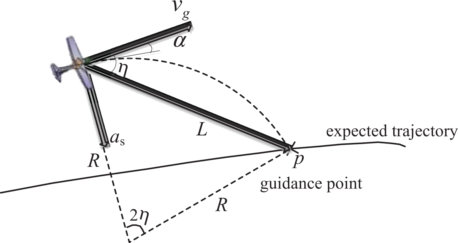
The basic principle of the nonlinear guidance law.

As shown in the figure, the lateral motion of the vehicle to follow the desired path is correlated to the lateral force and the corresponding acceleration a_s . To compute the required lateral acceleration, in a temporal guidance cycle, the motion of the UAV in the horizontal plane can be approximated as a circular trajectory.¹⁸ The radius can be computed from the geometry in Figure 3 as follows

R = \frac{L}{2 \times sin (η)}

And the lateral acceleration can be computed from Newton’s second law

a_{s} = \frac{v_{g}^{2}}{R}

So the expected lateral acceleration in equation (4) can be computed combining equations (2) and (3)

a_{s} = \frac{2 \times v_{g}^{2} \times sin (η)}{L}

As L is a constant parameter defined in advance, from the formula, the lateral acceleration is mainly determined by the ground speed v_g and the heading angle error η.

In another aspect, according to the balance requirement between weight and lift of the vehicle, the following formulas can be obtained as

{\begin{matrix} F_{L} \times cos (ϕ) = m g \\ F_{L} \times sin (ϕ) = m a_{s} \end{matrix}

where ϕ is the roll angle and F_L is the aerodynamic force perpendicular to the wing of the vehicle.

Consequently, combining equations (4) and (5), the roll angle command can be computed as follows

ϕ_{cmd} = arctan \frac{2 \times v_{g}^{2} \times sin (η)}{L g}

The generated command can be used in the inner loop. In another aspect, to make the vehicle fly flat in the plane, the coordinated turn is adopted, and the elevator should be used to compensate the fall of the vehicle during the rolling action.

The influence of the guidance distance

As the sole adjustable parameter in the nonlinear path following method (η is determined by L and the vehicle state), a significant relationship exists between L and the following result. So, in this section, a flight experiment will be provided firstly, to induce the impact of L, and the following research.

The experiment was carried out with the platform as shown in Figure 4. It is a commercial off-the-shelf model plane, and the length is about 1.6 m. The spin of the wing is about 2.4 m. The maximal takeoff weight is about 6.4 kg. For the experiment, the vehicle is equipped with an electric brushless motor and a propeller. The flight experiment is carried out based on an autopilot designed by the authors.

Figure 4.

The UAV for flight experiment. UAV: unmanned aerial vehicle.

During the experiment, the vehicle is required to follow a square trajectory, which is determined by the four waypoints marked 1234 in Figure 5. The expected flight speed (airspeed) is 15 m/s, and the southern wind is about 4 m/s during flight. The L is set 50 m at the first round and is increased 20 m once a loop, until 150 m. The flight trajectory is shown in Figure 5, and the cross-track error between waypoint 2 and waypoint 3 (considered as a stable following process) is shown in Figure 6.

Figure 5.

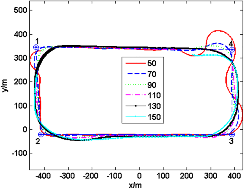
The flight results with different guidance distances during the experiment.

Figure 6.

The cross-track error during the stable flight process.

From Figures 5 and 6, during the stable following process, the precision is higher with a smaller L. However, during the turning process, oscillation may appear with a smaller L. This may be due to the fact that when L is very small, the vehicle starts to turn with very short distance to the current waypoint. In such case, the required turning radius may be smaller than the permitted value and may cause the vehicle to oscillate. However, if the vehicle starts to turn with a long distance to the current waypoint, the following precision may be worse than appropriate guidance distance, and the effect of executing special flight tasks may not be satisfied. This can be seen especially obvious from the results of the right-bottom corner (from waypoint 3 to waypoint 4) in Figure 5, where the vehicle is flying downwind, and the ground speed is larger (in such case, the permitted turning radius is bigger). So, how to determine an appropriate L and a suitable route switchover time (such as change the target waypoint from 3 to 4) automatically (according to the vehicle speed and attitude, etc.) is important for the vehicle to fly steadily and accurately. Based on the research below, the phenomenon of turning lead or lag is expected to be avoided.

The improved nonlinear path following method

Research of turning control during square trajectory with on-line transition trajectory generation method

Focusing on the problems above, an on-line transition trajectory generation method will be proposed in this section. The transition trajectory is expected to guarantee the vehicle choose appropriate route switchover time and fly steadily during intense maneuvers (such as the turning maneuver during square trajectory above, or the converging maneuver to expected trajectories with numerous errors at the initial state). Borrowing the ideas from the Dubins trajectory,¹⁹ the transition trajectory is mainly based on the circle with the minimal turning radius (corresponding to the vehicle speed), so to shorten the time needed for the transition process. To adapt to complicated circumstances, the transition trajectory should be generated on-line, rather than off-line. The main work of the on-line transition trajectory generation research includes:

the condition under which the transition trajectory exists;

the condition under which the vehicle should switch to/out the transition trajectory.

And the following discussion will be based on the typical situations, including the turning maneuver during the square trajectory and the converging maneuver to the expected circle trajectory with numerous errors at the initial state.

The typical situation of following a square trajectory can be seen in Figure 7. The vehicle is flying along the straight line AB and is to switch to the straight line BC. The temporal position of the vehicle is $O_{e} (x_{e}, y_{e})$ , and the heading is $ψ_{a}$ . v_g is the ground speed of the vehicle. The maximal allowed roll angle is $ϕ_{max}$ . According to the vehicle kinematics, the following formula (7) can be obtained as

R_{min} = \frac{v_{g}^{2}}{g \times tan (ϕ_{max})}

Figure 7.

Demonstration of generating the transition trajectory on-line.

From the geometric relationship in Figure 7, the constraint conditions for the transition trajectory can be summarized as follows

{\begin{array}{l} x_{0} = x_{e} + R_{min} \times sin (- \frac{π}{2} + ψ) \\ \begin{array}{l} y_{0} = y_{e} + R_{min} \times cos (- \frac{π}{2} + ψ) \\ \sqrt{{(x_{0} - x_{v})}^{2} + {(y_{0} - y_{v})}^{2}} \geq R_{min} \end{array} \end{array}

where $O (x_{0}, y_{0})$ is the center of the circle corresponding to the transition trajectory and $O_{v} (x_{v}, y_{v})$ is the projected point of $O (x_{0}, y_{0})$ on the straight line BC.

When the above formula is satisfied, the transition trajectory corresponding to a special turning radius exists, to realize the smooth switch from AB to BC. If the distance between $O (x_{0}, y_{0})$ and $O_{v} (x_{v}, y_{v})$ is just equal to $R_{min}$ , it just corresponds to $R_{min}$ .

So, with the object of shortening the time needed for the transition process, the condition for the vehicle to switch to the transition trajectory is that the distance between $O (x_{0}, y_{0})$ and the straight trajectory BC is $R_{min}$ . The condition for the vehicle to switch out the transition trajectory is that the vehicle reaches the $O_{v} (x_{v}, y_{v})$ position, or the vehicle rotates an angle at center of $2 β$ along the transition trajectory, where β is the angle between the vehicle heading at $O_{e} (x_{e}, y_{e})$ and the line of $O_{e} O_{v}$ .

Research of converging maneuver to expected circle trajectory with on-line transition trajectory generation method

The vehicle is required to follow a circle trajectory with the counterclockwise direction. The circle center is O, and the circle radius is R. The temporal position for the vehicle is $O_{e} (x_{e}, y_{e})$ , and the heading angle is $ψ_{a}$ . The cross-track error between the vehicle and the circle is $d_{cr}$ . To realize a smooth switch from the temporal state to the circle, the transition trajectory should be designed as follows:

The cross-track error $d_{cr} > 0$ , and the geometric relationship is shown in Figure 8.

Figure 8.

Demonstration of generating the transition trajectory for converging to the circle with circumcircle.

As shown in Figure 8, the center of the transition circle corresponding to the minimal turning radius can be obtained as

{\begin{array}{l} x^{'} = x_{e} + R_{min} \times sin (\frac{π}{2} + ψ) \\ y^{'} = y_{e} + R_{min} \times cos (\frac{π}{2} + ψ) \end{array}

The line from O to $O^{'}$ intersects with the transition circle at point O_v . The distance between O and $O^{'}$ is computed as follows

d^{'} = \sqrt{{(x_{0} - x^{'})}^{2} + {(y_{0} - y^{'})}^{2}}

When the following formula (11) is satisfied, the transition trajectory from the temporal state of the vehicle to the circle exists. When the equality is satisfied, it just corresponds to the critical state and is the condition for the vehicle to switch to the transition trajectory

d^{'} \geq R_{min} + R

(2) The cross-track error $d_{cr} < 0$ , and the geometric relationship is shown in Figure 9.

Figure 9.

Demonstration of generating the transition trajectory for converging to the circle trajectory with incircle.

The deduction is similar to the process above, and the condition for the vehicle to switch to the transition trajectory is as follows

d^{'} = R - R_{min}

Obviously, the solution only exists when $R \geq R_{min}$ .

Similar to the turning control during square trajectory, the condition for the vehicle to switch out the transition is that the vehicle reaches the point of tangency $O_{v} (x_{v}, y_{v})$ , or the vehicle rotates an angle of $2 β$ along the transition trajectory, where β is the angle between the vehicle heading at $O_{e} (x_{e}, y_{e})$ and the line of $O_{e} O_{v}$ .

The improved nonlinear guidance method with adaptive guidance distance

The discussion above is mainly focused on the on-line transition trajectory generation problem. The transition trajectory is designed to solve the route switchover opportunity problem and the smooth transition of intense maneuvers (such as the turning maneuver in Figure 5). How to guarantee the vehicle follow the designed trajectory, and fly steadily is important, especially when the flying circumstance is complicated. The nonlinear guidance algorithm can be applied to many situations.⁵ However, the guidance distance is crucial to the algorithm, and this can be seen from the results in Figure 6. When the VTP is too close to the vehicle, some oscillation may appear; when the VTP is too far away from the vehicle, the following precision may not be satisfied. So, the nonlinear guidance algorithm is to be improved with an adaptive guidance distance algorithm below. Through the adaptive guidance distance method, the vehicle is expected to fly accurately and steadily.

The approximate linear model of the nonlinear guidance algorithm is derived in the studies of Kothari et al.¹⁰ and Park et al.¹¹ as follows

a_{c} \approx 2 \frac{v}{L} ({\dot{d}}_{cr} + \frac{v}{L} d_{cr})

And it is similar to a linear PD controller. From the formula, the gain of the controller is mainly determined by the ratio between the vehicle speed v and the guidance distance L. From the theory of traditional control system, when the vehicle speed v is constant, a smaller L equals to a high control gain, and the controller would response to the cross-track error quickly and accurately (in appropriate scope). But if the L is too small, the gain of the controller may be oversize, and some overshoot or even oscillation may appear. So, to a special vehicle speed, the lower limit of L should exist.

From the study of Park et al.,^11,12 the nonlinear guidance algorithm is approximated to a second-order system, and the damping ratio is $ζ = \frac{1}{\sqrt{2}}$ , the natural frequency is $ω_{n} = \frac{\sqrt{2} v}{L}$ . So, the bandwidth of the nonlinear guidance algorithm is computed as follows

ω_{guidance} = \frac{\sqrt{2} V}{L}

As a whole system, the dynamic character of the guidance algorithm should be within the scope of the dynamic character of vehicles, so the vehicle is able to follow the guidance command. From Shannon’s theorems, the bandwidth of the guidance algorithm should be less than or equal to one half of the bandwidth of the vehicles (including the control system). So, formula (15) can be obtained as

ω_{guidance} < \frac{1}{2} ω_{UAV}

From equations (14) and (15), the lower limit of L can be obtained as

L_{min} = \frac{2 \sqrt{2} v}{ω_{UAV}}

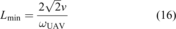
From equation (16), the lower limit of the guidance distance corresponding to a fixed vehicle speed is determined by the bandwidth of the vehicle $ω_{UAV}$ . To a special vehicle with a fixed speed, the appropriate lower limit can be determined in advance. When the circumstance is simple, the lower limit value can be used for path following directly. However, if the wind is disorderly, the vehicle may be blown away from the expected trajectory and the speed is varied. In such case, the lower limit value may result to small oscillation and affect the stability of the vehicle. So, the lower limit is not enough in such case. The appropriate value for L should be chosen in every control cycle, and an algorithm with adaptive guidance distance will be proposed below.

In another aspect, the real-time requirement is important for a control system of a vehicle. So, the upper limit of L is determined by the permitted optimization time automatically. Assuming the control period is T, and the permitted optimization time for L is about t_a . Based on $L_{min}$ , the guidance distance is increased by a fixed step $Δ L$ iteratively in T, and the optimal value is chosen based on a designed criterion. When the optimization time is over t_a , the process stops, and the upper limit is determined automatically. From the simulation results, for the researched low-speed vehicles up to now (15–30 m/s), the reasonable upper limit of L is about 80–150 m over the lower limit. When the L is out of the scope, the following accuracy may decline severely. In another aspect, the simulation results can be taken into consideration synthetically, to determine the scope of the guidance distance.

The detailed algorithm

With the scope of the guidance distance, a path following method with an adaptive guidance distance is designed, and the basic demonstration is shown in Figure 10.

Figure 10.

Demonstration of the guidance algorithm with an adaptive guidance distance.

Assuming the temporal position of the vehicle is O_e , and the ground speed is v_g . The heading of the vehicle is $ψ_{a}$ . The path following algorithm with adaptive guidance distance is mainly composed of the following steps:

From the lower limit of L, the guidance distance is increased by $Δ L$ every time and indexed as $L_{0}, L_{1}, L_{2}, ..., L_{n}$ (written as $L_{j}, j = 0, 1, 2, ..., n$ below). The corresponding VTPs are denoted as $O_{ref 0}, O_{ref 1}, O_{ref 2}, ..., O_{ref n}$ .

For every sampled guidance distance, a predicted trajectory is generated with the temporal vehicle position/heading and the VTP. As in the path following process, only the kinematic model is concerned, the predicted trajectory is approximated as an arc of a circle. As shown in Figure 10, the centers of the predicted trajectory are $P_{0}, P_{1}, P_{1}, ..., P_{n}$ and the radii are $R_{0}, R_{1}, R_{1}, ..., R_{n}$ .

Based on the predicted trajectories and the expected trajectory, a criterion is designed to evaluate the different guidance distances. The criterion is designed from the concepts of overshoot and converging rapidity in traditional control theory and would be given in detail below. The optimal guidance distance and the corresponding VTP are chosen to lead the vehicle follow the expected trajectory.

In every control cycle, the (1)–(3) steps above are executed to find the optimal guidance parameter for path following and to improve the following accuracy and stability.

The criterion for guidance distance evaluating

In the path following method with an adaptive guidance distance above, the criterion to evaluate the guidance distances is crucial. The following performance is affected directly by the criterion. Borrowing the ideas of overshoot and converging rapidity in traditional control theory, the criterion is designed as shown in Figure 11.

Figure 11.

Demonstration of the criterion for guidance distance evaluating.

When the guidance distance is L, the VTP is $O_{ref}$ . The radius of the predicted trajectory is R, and the angle at the center is $2 η$ . The projected point of the temporal position O_e on the expected trajectory is $O_{e}^{'}$ , and the length of $O_{e} O_{e}^{'}$ is the cross-track error.

In the triangle $Δ O_{e} O_{e}^{'} O_{ref}$ , $O_{e} O_{e}'$ is a denotation of the cross-track error, and $O_{e}^{'} O_{ref}$ denotes the length under which the vehicle should go through to converge to the expected trajectory. The product of $O_{e} O_{e}'$ and $O_{e}^{'} O_{ref}$ can be seen as a representation of the converge rapidity. So, in the article, the square of $Δ O_{e} O_{e}^{'} O_{ref}$ is defined as the criterion of the converge rapidity to the expected trajectory.

In another aspect, there is an angle error θ between the predicted trajectory and the expected trajectory at point $O_{ref}$ , as shown in Figure 11. The angle includes the information of the overshoot by the predicted trajectory. However, as the units of the angle and the cross-track error are different, the normalization of the two variables may be difficult. So, in the article, with the angle error θ, it is assumed that the vehicle is to eliminate the error with the minimal turning radius, as shown in Figure 11, the arc of a circle $O_{ref} O_{ref}^{'}$ . With the arc $O_{ref} O_{ref}^{'}$ , the generated cross-track error is $d_{cr}^{'}$ , and it is used as another representation of the overshoot corresponding to the guidance distance L. Detailed computation of $d_{cr}^{'}$ is given below.

The heading of the predicted trajectory at point $O_{ref}$ is as follows

θ_{1} = ψ + 2 η

Assuming the heading of the expected trajectory at point $O_{ref}$ is $θ_{2}$ , and it is determined by the expected trajectory. So, the angle error θ can be computed as follows

θ_{d} = | θ_{1} - θ_{2} |

And the cross-track error $d_{cr}^{'}$ is calculated as follows

d_{cr}^{'} = R_{min} (1 - c o s θ_{d})

With the terms of the square of $Δ O_{e} O_{e}^{'} O_{ref}$ and $d_{cr}^{'}$ above, the criterion is defined as follows

Q = w_{1} \times L \times d_{cr} + w_{2} \times R_{min} \times d_{cr}^{'}

where $L \times d_{cr}$ is an approximation of the square of $Δ O_{e} O_{e}^{'} O_{ref}$ , and $R_{min}$ is added in equation (20) to unify the two terms. w ₁ and w ₂ are the weights corresponding to converging rapidity and overshoot, and $w_{1} + w_{2} = 1$ . In the simulation results, w ₁ is designed as follows

ω_{1} = {\begin{array}{l} 0; & d_{cr} \geq L_{min} \\ (1 - \frac{d_{cr} - L_{min} / n_{0}}{L_{min} - L_{min} / n_{0}}) \times 0.8; & L_{min} > d_{cr} \geq L_{min} / n_{0} \\ 0.8; & d_{cr} \leq L_{min} / n_{0} \end{array}

where $n_{0} \approx 5 - 10$ . The best guidance distance is chosen as follows

{\begin{cases} P_{best} = min (P_{j}), j = 1, 2... n \\ J = {j | min (P_{j})} \\ L_{best} = L_{min} + J \times Δ L \end{cases}

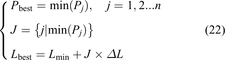
where P_j are the costs corresponding to different guidance distances, and $P_{best}$ is the best one. $Δ L$ is the variation of the guidance distance to every sampling cycle, and J is the sampling value of the optimal guidance distance.

One point to mention is that, when $R < R_{min}$ , the cost value is infinite.

Simulation results

The on-line transition trajectory generation and following

To verify the performance of the proposed method, some simulations were carried out. The simulation experiments were taken on the PC computer with Windows 10 System. The CPU of the computer is Intel(R) Core(TM) i7-8750H. The RAM of the computer is 8G. The Visual Studio 11 environment was used to model the vehicle and realize the control system. The simulation results of transition trajectory generation on-line and following are shown in Figure 12. The initial position of the vehicle is $(0, 0)$ and the heading is $\frac{π}{2}$ . The vehicle is flying along the line of $y = 0$ with a speed $v = 15 m/s$ . The expected trajectory is composed of a parallelogram ABCD and a circle with radius 90 m. The maximal roll angle is defined as 35°. The control period of the inner loop is 50 Hz.

Figure 12.

Simulation results with and without the transition trajectory.

From the parameters above, the minimal turning radius is $R_{min} \approx 70 m$ . The bandwidth of the vehicle is about $ω_{UAV} \approx 0.8$ through theory analysis and model identification. So, from equation (16), $L_{min} \approx 50 m$ . As the inner loop control period is 50 Hz, the permitted time for the guidance distance optimization should be less than 10 ms, $t_{a} = 0.01 s$ . So, the variation of the guidance distance $Δ L = 5 m$ and $n_{0} = 5$ . From the results in Figure 12, the condition to generate the transition trajectory is satisfied, and the following results with different methods are given.

Firstly, in Figure 12, the red line denotes the result based on transition trajectory generation and the path following method with guidance distance of lower limit. The blue line is without transition trajectory generation and based on the path following method with the guidance distance of lower limit. From the results, without the transition trajectory, the path following method can guide the vehicle fly steadily during turning with obtuse angles. But oscillation may appear during the turn. However, the generation of the transition trajectory can well solve the oscillation problem during intense maneuvers, such as turning with acute angles. The vehicle can converge to the circle trajectory smoothly, with the guidance distance of lower limit.

In another aspect, from the roll angles during the turning process in Figure 13, with the transition trajectory, the vehicle can keep a steadier roll angle than without the transition trajectory, as shown by the red line and the blue line. This can be seen obviously from the roll angle at about 35s, during the first turn. For the other turns, as the result without the transition trajectory is oscillating almost all the time, the advantage of the transition trajectory is remarkable. From the results of the red line and the green line, the roll angle by the path following method with an adaptive guidance distance is smoother. This is the result of the adaptation of the guidance distance, as shown in Figure 14. From Figure 14, most of the time, the guidance distances are similar between the path following method with an adaptive guidance distance and with fixed guidance distance. But at the end of the transition trajectory following process, the guidance distance is longer and improves the smooth of the roll angle. This can be seen more obviously from the simulation results below.

Figure 13.

The roll angle during the turning process.

Figure 14.

The guidance distance during the simulation.

Simulation results with adaptive guidance distance

In the simulation, the vehicle is to follow a circle with center at $(0, 0)$ and radius 200 m. The desired speed is 15 m/s. However, due to the disturbance of wind, the vehicle is blown away from the desired circle, as shown in Figure 15. The path following results with an adaptive guidance distance and a fixed guidance distance are also shown in the figure.

Figure 15.

Simulation results of the path following method with adaptive guidance distance and fixed guidance distance.

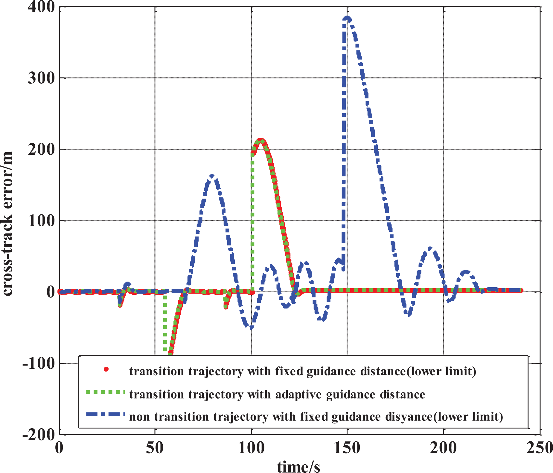
From the simulation results, when the vehicle is deviated from the expected trajectory, small oscillation may appear based on the path following method with a fixed guidance distance. This can be seen obviously from the cross-track error in Figure 16. From Figure 16, the time used for the vehicle to converge to the expected trajectory is about 31s, based on the fixed guidance distance. However, the time is shortened to 25s, based on the adaptive guidance distance. The maximal cross-track error based on the fixed guidance distance is larger than 3 m, while the error is smaller than 1 m with an adaptive guidance distance.

Figure 16.

The cross-track error during the simulation.

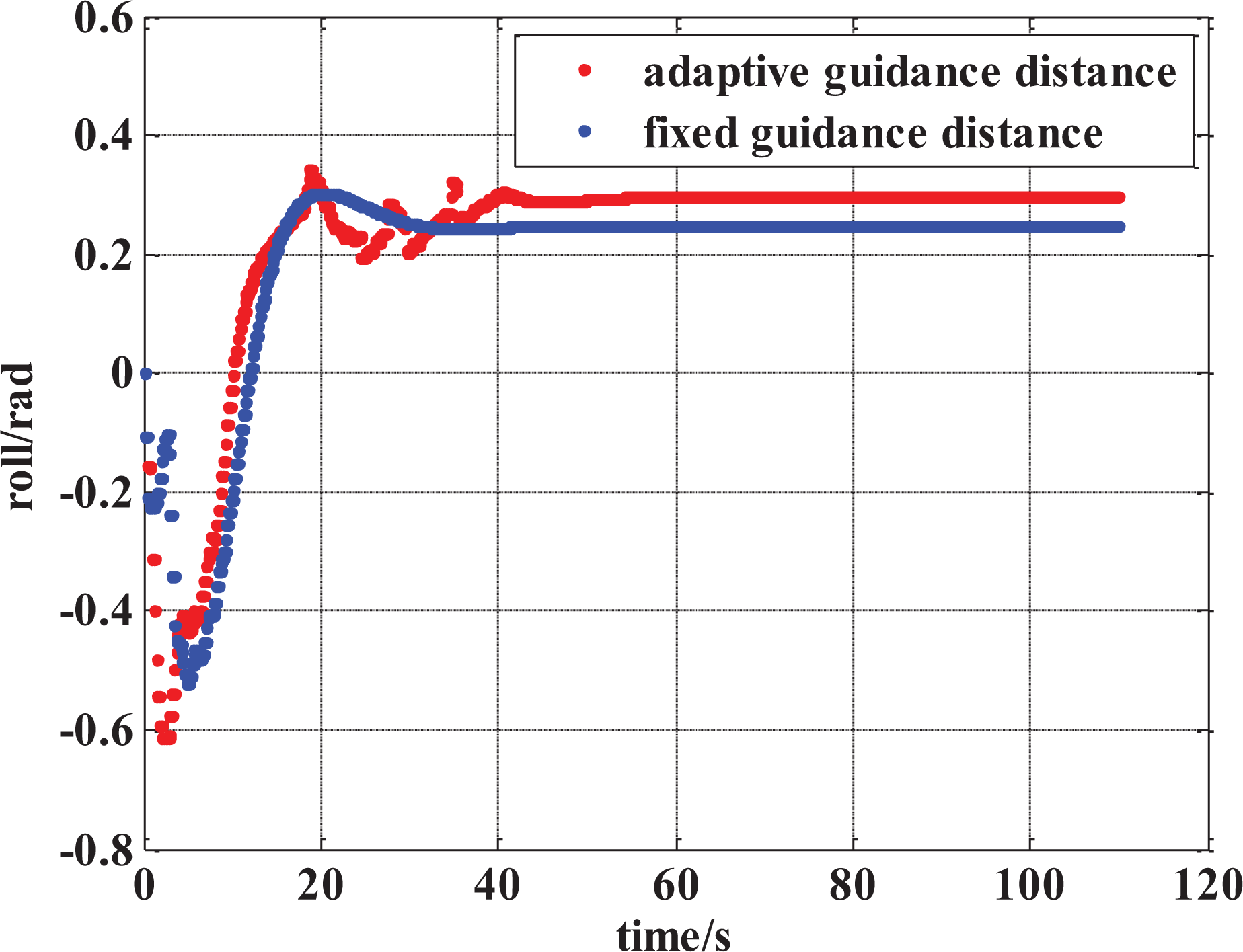
In another aspect, from the results in Figure 17, the roll angle based on the adaptive guidance distance method is smoother than that with a fixed guidance distance. With a fixed guidance distance, the roll angle may oscillate at the initial stage. From the guidance distance in Figure 18, during the converging process, the guidance distance is larger. This is consistent with the analysis above in formula (13): When the guidance distance is smaller, the control gain would be larger and some overshoot may appear. So, the adaptive guidance distance method is similar to a gain-scheduling method in the control theory and is important to guarantee the stability of the controller.

Figure 17.

The roll angle during the simulation.

Figure 18.

The guidance distance during the simulation.

So, based on the simulation results above, the on-line transition trajectory generation method can well solve the stability problem during intense maneuvers, such as acute turnings or converging to trajectories under numerous errors at the initial state (including the position and heading errors). The path following method with an adaptive guidance distance is effective to conquer small oscillation during converging to the desired trajectory with a limited error. The combination of the two methods can improve the performance of the nonlinear path following method significantly.

Flight experiments

To verify the effectiveness of the proposed method, flight experiments were carried out, based on a platform shown in Figure 19. The platform named FX-0501 is aimed to be an all-terrain multipurpose UAV. In order to adapt to the all-terrain requirement, the vehicle is designed to take off by the elastic rope catapult method and to automatic recovery by a net collision system. The elastic rope catapult takeoff system and the net recovery system can be seen in Figure 19 ²⁰. The length of the vehicle is about 2.0 m and the wing span is about 3.2 m. The vehicle is driven by a 3W 28i engine and is expected to fly about 10 h when the fuel tank is full. The flight time is enough to test the performance of the control method. As shown in Figure 20, in the automatic net recovery system, the width of the net is about 5.0 m, and the length is about 9.0 m. So, to realize a safe recovery of the UAV, the requirement of the path following accuracy is very strict.

Figure 19.

(a) The unmanned aerial vehicle during the flight experiments and (b) the takeoff and recovery method of the unmanned aerial vehicle.

Figure 20.

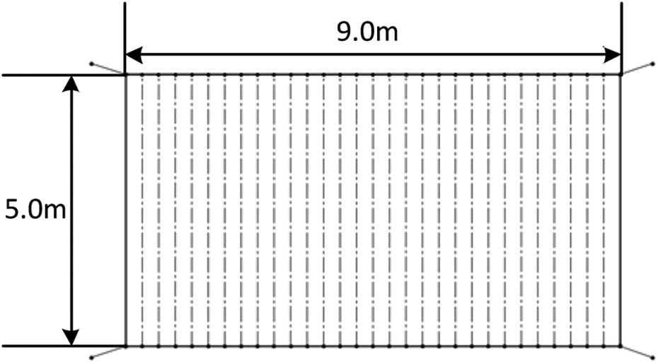
The size of the net.

To achieve an automatic recovery of the UAV reliably, the proposed method is adopted. The experiment is carried out repeatedly to verify the effectiveness and robustness of the proposed method. One of the experiment results can be seen in Figure 21. The detailed trajectory of the vehicle and the expected net position is shown in Figure 21(a), and the variation of the height of the vehicle to the ground is shown in Figure 21(b).

Figure 21.

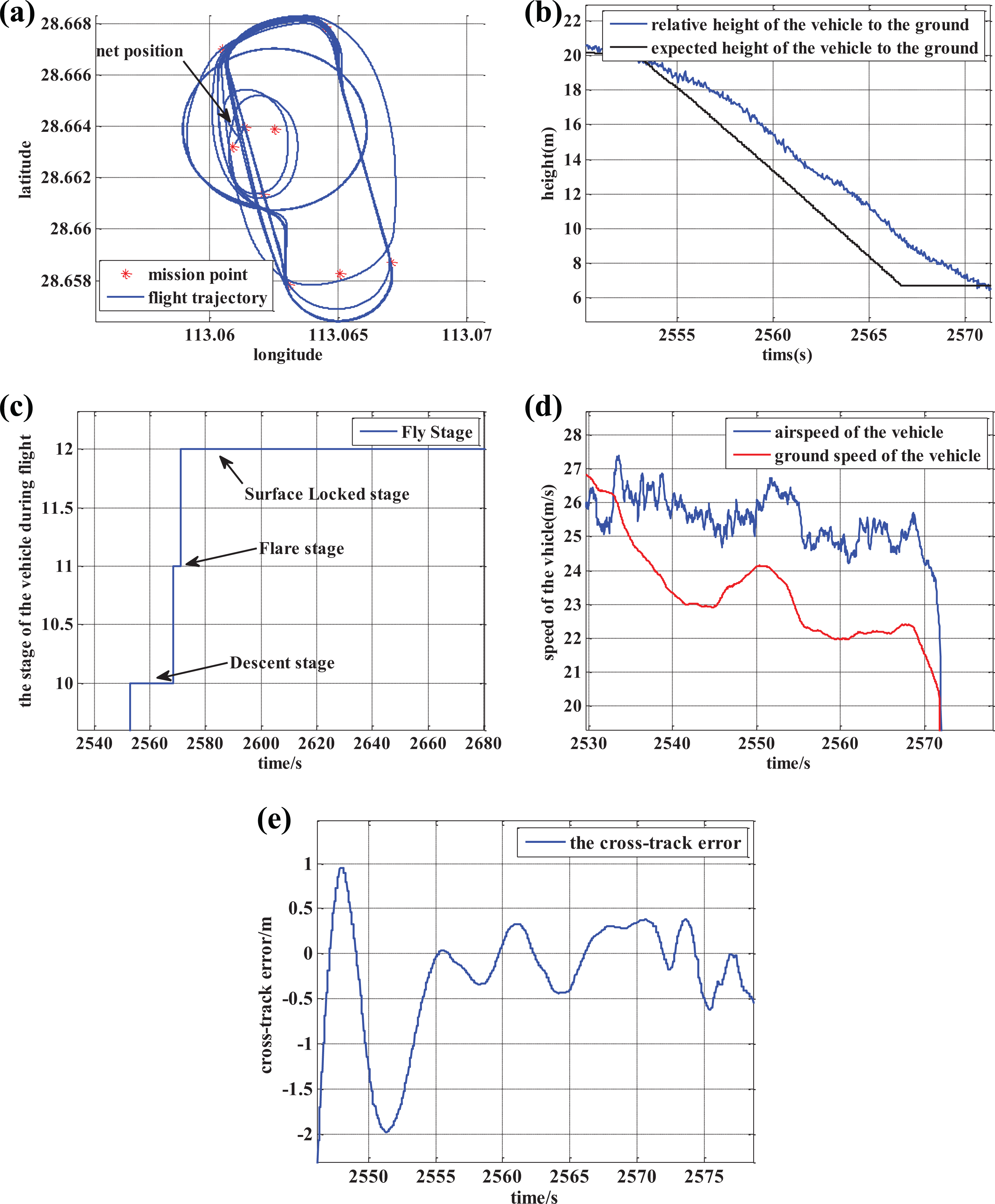
The experiment results during the net recovery process: (a) the flight trajectory of the vehicle, (b) the height of the vehicle relative to the ground, (c) the fly stage of the vehicle, (d) the speed of the vehicle, and (e) the cross-track error during the net recovery process.

From the experiment results, as shown in Figure 21(b), when the vehicle comes into the net recovery process, the expected height of the vehicle changes from about 20 m to the height of the net (about 6.8 m). From Figure 21(e), although the cross-track error is larger than 1.5 m when the vehicle starts to fly toward the net (at about 2552 s), it converges to the scope of ±0.5 m quickly (at about 2555 s). As the width of the net is 5 m, and the wing span is 3.2 m, the cross-track error is sufficient for the vehicle to collide safely with the net. One point to mention is that, from Figure 21(c), to realize the net recovery aim, the flight of the vehicle during the recovery process is divided into a descent stage, a flare stage, and a surface locked stage, which is easy for the design of the inner loop control algorithms. The detailed flight process of the vehicle can be seen in Figure 22.

Figure 22.

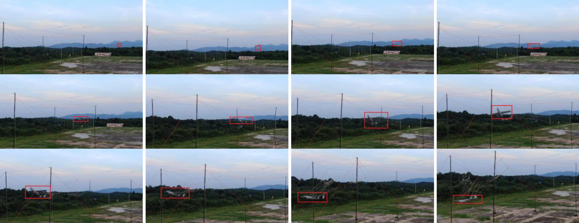
The detailed demonstration of the automatic net recovery process. The UAV flies along the expected trajectory and finally collides with the recovery net. The cross-track error is smaller than 1 m, which is sufficient to satisfy the requirement of the net recovery process. The detailed position of the vehicle in each frame is shown by the red square.

In another aspect, from Figure 21(d), the ground speed of the vehicle is smaller than the airspeed. So, the result in Figure 21 is an upwind case. The experiment results in downwind case can be seen in Figure 23. The ground speed of the vehicle is larger than the airspeed, as shown in Figure 23(d). The detailed trajectory of the vehicle and the expected net position are shown in Figure 23(a), and the variation of the height of the vehicle to the ground is shown in Figure 23(b). From Figure 23(e), the proposed method can adapt to different situations, which is important for the method to be used widely. The stages in Figure 23(c) are just similar to Figure 21(c).

Figure 23.

The experiment results during the net recovery process in downwind situation: (a) the flight trajectory of the vehicle, (b) the height of the vehicle relative to the ground, (c) the fly stage of the vehicle, (d) the speed of the vehicle, and (e) the cross-track error during the net recovery process.

Conclusions and future work

Based on the nonlinear path following method, research to improve the stability and accuracy was carried out and some achievements have been acquired:

The on-line transition trajectory generation method was proposed to solve the oscillation problem appeared during intense maneuvers. Firstly, from the results of the flight experiment, the importance of the route switchover time and the transition trajectory was deduced. Secondly, for typical maneuvers, such as acute turning control during square trajectories and converging maneuvers to an expected circle trajectory under numerous initial errors, the condition under which transition trajectory exists was analyzed, and the time to switch to/out the transition trajectory was determined automatically.

The path following method with an adaptive guidance distance was proposed, with a criterion incorporating the rapidity and overshoot concepts from the traditional control theory. The adaptive guidance distance method was designed to solve the oscillation problem during following process (the initial following error may be caused by disturbance such as wind) and improve the following stability and accuracy.

The proposed method was verified through simulations and flight experiments. From the simulation results, the transition trajectory can conquer the oscillation problem during turning with acute angles, and the vehicle can converge to the expected trajectory steadily, even with numerous initial errors. The maximal cross-track error based on a fixed guidance distance is larger than 3 m, while the error is smaller than 1 m with an adaptive guidance distance, when the vehicle is converged to the expected trajectory. When some following errors appear, the adaptive guidance distance method can improve the following stability and accuracy. This is important for the vehicle to fly safely. From the experiment results, the proposed method can guarantee the path following accuracy in different situations (such as in upwind or downwind cases). The path following error is smaller than 1.0 m when it is converged (in downwind or upwind situations), just as consistent with the simulation results. This is important to satisfy the strict requirement of automatic net recovery of UAVs.

Up to now, in the proposed path following method, the chosen of the guidance distance is mainly upon the predicted trajectory with a kinematic model and only one step prediction. To improve the accuracy, how to adopt the dynamical model and realization prediction with multisteps is to be researched in future.

Footnotes

Acknowledgments

The authors would like to thank the other person in the group to carry out the flight experiments. In another aspect, the authors would like to thank anonymous reviewers for their constructive comments and suggestions that improved the article.

Declaration of conflicting interests

The author(s) declared no potential conflicts of interest with respect to the research, authorship, and/or publication of this article.

Funding

The author(s) received no financial support for the research, authorship, and/or publication of this article.

ORCID iDs

Qingyang Chen

Yafei Lu

References

Jia-ming

Qing

Nong

, et al. Nonlinear path-following method for fixed-wing unmanned aerial vehicles. J Zhejiang Univ Sci C 2013; 14(2): 125–137.

Lekkas

Fossen

. Integral LOS path following for curved paths based on a monotone cubic Hermite spline parametrization. IEEE Trans Control Syst Technol 2014; 22(6): 2287–2301.

Conte

Duranti

Merz

. Dynamic 3D path following for an autonomous helicopter. In: Proceedings of the fifth IFAC symposium on intelligent autonomous vehicles, Oxford, UK, 2004, pp. 473–478.

Ambrosino

Ariola

Ciniglio

, et al. Path generation and tracking in 3-D for UAVs. IEEE Trans Control Syst Technol 2009; 17(4): 980–988.

Osborne

Rysdyk

Waypoint guidance for small UAVs in wind. In: Proceedings of the AIAA infotech aerospace, Arlington, VA, USA, 2005, pp. 459–470.

Fossen

Breivik

Skjetne

. Line-of-sight path following of underactuated marine craft. In: Proceedings of the sixth IFAC conference on manoeuvring control marine craft, Girona, Spain, 17–19 September 2003, pp. 244–249.

Papoulias

FA.

Stability considerations of guidance and control laws for autonomous underwater vehicles in the horizontal plane. In: Proceedings of the seventh international symposium on unmanned untethered vehicle technology, Durham, NH, USA, 1991, pp. 140–158.

Rysdyk

. UAV path following for constant line-of-sight. In: The second AIAA unmanned unlimited systems, technologies operations aerospace, land sea conference, San Diego, CA, USA, 15–18 September 2003.

Rysdyk

. Unmanned aerial vehicle path following for target observation in wind. J Guid Control Dyn 2006; 29(5): 1092–1100.

10.

Kothari

Postlethwaite

Da-Wei

. UAV path following in windy urban environments. J Intell Robot Syst 2014; 74: 1013–1028.

11.

Park

Deysty

Howz

. A new nonlinear guidance logic for trajectory tracking. In: AIAA guidance, navigation, and control conference and exhibit, Providence, RI, USA, 1984, pp. 941–956.

12.

Park

Deystt

Howz

. Performance and Lyapunov stability of a nonlinear path-following guidance method. J Guid Control Dyn 2007; 30(6): 1718–1728.

13.

Rhee

Park

Chang-Kyung

. A tight path following algorithm of an UAS based on PID control. In: SICE annual conference 2010, Taipei, Taiwan, 2010, pp. 1270–1273.

14.

Sujit

Saripall

Sousa

. Unmanned aerial vehicle path following: a survey and analysis of algorithms for fixed-wing unmanned aerial vehicles. IEEE Control Syst 2014; 34: 42–59.

15.

Zhao

Wang

Zhang

, et al. Model predictive control based integral line-of-sight curved path following for unmanned aerial vehicle. In: AIAA guidance, navigation, and control conference, Grapevine, TX, USA, 2017, pp. 1–13.

16.

Xavier

Natassya

BFS

Kalinka

RLJCB

. Path-following algorithms comparison using Software-in-the-Loop simulations for UAVs. In: 2019 Workshop on communications in critical embedded systems, Barcelona, Spain, 29 June–3 July 2019, pp. 1216–1221.

17.

Saurav

Sohil

Ghosh

. Variable L1 guidance strategy for path following of UAVs. In: 2020 International conference on unmanned aircraft systems (ICUAS), Athens, Greece, 1–4 September 2020, pp. 1518–1524.

18.

Chen

. UAVs formation flight control based on following of the guidance points. In: Proceedings of 2016 IEEE Chinese guidance, navigation and control conference, Nanjing, China, August 12-14, 2016, 2016, pp. 730–735.

19.

Dubins

. On plane curves with curvature. Pacific J Math 1961; 11(2): 471–481.

20.

Hanyi

Yafei

Zhongxi

, et al. 3D Dubins net-recovery path planning for fixed wing UAV. In: The 30th Chinese control and decision conference, Shenyang, China, 9–11 June 2018, 2018, pp. 604–610.

An improved nonlinear path following method with on-line transition trajectory generation for fixed-wing unmanned aerial vehicles

Abstract

Keywords

Introduction

The nonlinear path following method

Flight control system

UAV navigation model

The nonlinear path following method

The influence of the guidance distance

The improved nonlinear path following method

Research of turning control during square trajectory with on-line transition trajectory generation method

Research of converging maneuver to expected circle trajectory with on-line transition trajectory generation method

The improved nonlinear guidance method with adaptive guidance distance

The detailed algorithm

The criterion for guidance distance evaluating

Simulation results

The on-line transition trajectory generation and following

Simulation results with adaptive guidance distance

Flight experiments

Conclusions and future work

Footnotes

Acknowledgments

Declaration of conflicting interests

Funding

ORCID iDs

References