Sage Journals: Discover world-class research

Abstract

The inverse kinematics problem involves the study that the inverse kinematics solver needs to calculate the values of the joint variables given the desired pose of the end-effector of a robot. However, to apply to seven-degree-of-freedom robots with arbitrary configuration, analytical methods need to fix one joint and set an increment when the current value fails to solve the inverse kinematics problem. Although numerical methods based on inverse differential kinematics are efficient in solving the inverse kinematics problem of seven-degree-of-freedom robots with arbitrary geometric parameters, they are deficient in numerical stability and time-consuming for convergence to one solution governed by the initial guess. In order to reduce the execution time of an inverse kinematics solver, this article introduces a speedup method for analytical and numerical methods, which can improve their performance.

Keywords

Robot kinematics speedup method Newton–Raphson method Levenberg–Marquardt algorithm sequential quadratic programming inverse kinematics

Introduction

In order to place its end-effector exactly at a desired position and orientation in Cartesian space, a serial-chain robot needs to possess no less than six degrees of freedom (DOFs). A 7-DOF robot has one more redundant DOF than it requires for positioning the end-effector in Cartesian space. A 7-DOF robot has more practical significance in applications as it has some advantages. For example, it can provide greater flexibility and reliability when executing tasks and avoid obstacles in complex and unknown work environments. But unfortunately, it is arduous to find the solution of inverse kinematics (IK) for a redundant robot in real time. How to solve the inverse kinematics problem (IKP) of a redundant serial-chain robot has been and remains quite challenging in robotics research and applications.

Generally speaking, there exist analytical methods and numerical methods to solve the IKP of redundant robots.¹ Because the IK solver must be pre-built, an analytical IK solution method cannot be generalized to the cases where a robot configuration changes and a tool is mounted at the end. Numerical methods are widely used to solve the IKP of various configurations. However, due to the limitation of the number of iterations and the setting of convergence conditions, these IK solution methods are sometimes not feasible. Most numerical IK solution methods use the Newton–Raphson (NR) algorithm² or similar to iterate until they find a solution. Compared with analytical methods, numerical methods are reasonable in theory, and they take a long time to find one IK solution. Sometimes, the precision of the found solution is low, and even the phenomenon occurs that the IKP cannot be solved correctly. Scholars have developed many methods to accelerate the calculation of Jacobian and matrix inversion and optimize numerical methods to improve solution efficiency. Many methods are developed according to the Denavit–Hartenberg (D-H) parameters of robots, but there are methods based on screw transforms³ and exponential rotational matrices,⁴ which arise from the explicit physical interpretation of the mechanism with Euler wrist and can be easily realized. The IKP becomes more complicated when obstacles in the workspace impose collision avoidance constraints. Convex Iteration for Distance-Geometric Inverse Kinematics algorithm can solve the convex feasibility problem whose low-rank feasible points provide exact IK solutions for complex workspace constraints.⁵

For redundant robots, the analytical IK solution needs one joint fixed and then solves other joint rotation angles. Concerning the initial fixed joint angle value, the solution may fail. If it happens, an increment will add to the initial value until the solution succeeds within the time limit. Thus, more precisely to say, the fixed joint is free to change its value. For specific mechanisms, such as manipulators with Euler wrist, using dual quaternions can obtain a very compact formulation for closed-form solutions.⁶ As to the numerical IK solution, a set of initial joint angles is required to compute the first Jacobian or as a seed state to start an iterative search. Prior to finishing the solving process, the number of iterations cannot be determined. To reach a particular precision, this kind of approach is computationally expensive in many cases, which can be numerically unstable. Although state-of-the-art algorithms have reduced inverse solution computation time to milliseconds or even microseconds, the challenge of computational efficiency in real-time robot motion planning still exists, especially for complex robot configurations. In this article, we propose a speedup solution to the IKP of a 7-DOF redundant robot, which can reduce the computational time when applying analytical and numerical methods for the IKP and improve the success rate of the analytical method.

Methods

Solving the IKP of redundant robots is a problem of nonlinear mapping from robot operating space to joint space. It has to seek the numerical solution of nonlinear transcendental equations.⁷ At present, methods to solve the IKP of redundant DOF robots are mainly numerical, such as pseudo-inverse of Jacobian methods,⁸ extended Jacobian methods,⁹ task-space augmentation methods,¹⁰ gradient projection methods,¹¹ damped least square methods,¹² and weighted least-norm methods.¹³ Besides, there are analytical methods to solve the IKP of redundant robots with specific geometric properties, such as solution algorithms based on screw theory,¹⁴ geometric methods for robots with unique geometric features,^15,16 and the analytical approach by fixing a certain DOF.¹⁷

We denote the configuration space of an n-joint, serial-link articulated robot as Q, which consists of n-tuples element $\vec{q} = {(θ_{1}, θ_{2}, \dots, θ_{n})}^{T} \in ℝ^{n}$ , each $θ_{i}$ representing the ith joint value of the robot, and its operating space as X, which consists of 6-tuples $\vec{x} \in ℝ^{6}$ with three translation variables p_x , p_y , and p_z and three rotation angle variables α, $β$ , and $γ$ . Then, a forward kinematic equation of this robot is represented as

\vec{x} = FK (\vec{q}), \vec{x} \in X, \vec{q} \in Q

Function $FK : Q \to X$ is differentiable. For each $\vec{x}$ in operating space, according to the IK equation $IK (\vec{x}) = {\vec{q} | \vec{x} = FK (\vec{q})}$ , there exist infinite sets of joint values $\vec{q}$ corresponding to one same point $\vec{x}$ in operation space. In other words, the IK equation will have infinite solutions.

IKfast approach

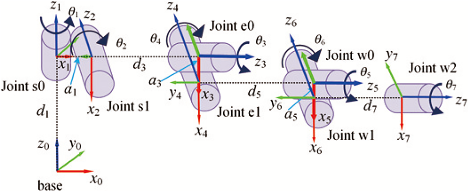
We can use the D-H convention, kinematic chains, or unified robot description format (URDF) to represent the geometry of a robotic mechanism. An articulated joint has a revolute joint variable and other constant parameters. Regardless of how to represent the geometry of a robot, the coordinate system of one of its joints relative to the reference frame can be defined as $A_{i} = T_{i} J_{i}$ , where T_i is a constant affine transformation computed by the invariant geometrical parameter and J_i is a transformation depending on variable $θ_{i}$ , which is a rotation angle around an arbitrary axis ${\vec{v}}_{i} (v_{i, x}, v_{i, y}, v_{i, z})$

J_{i} (θ_{i}) = I_{4 \times 4} + sin θ_{i} \hat{ω} + (1 - cos θ_{i}) {\hat{ω}}^{2}

In equation (2), $\hat{ω}$ is a $4 \times 4$ skew matrix defined by

\hat{ω} = [\begin{matrix} 0 & - v_{i, z} & v_{i, y} & 0 \\ v_{i, z} & 0 & - v_{i, x} & 0 \\ - v_{i, y} & v_{i, x} & 0 & 0 \\ 0 & 0 & 0 & 0 \end{matrix}]

Thus, the transformation of the end-effector can be formulated by continuous multiplication of the fundamental transformation: $T_{e e} = A_{1} A_{2} \dots A_{n}$ . With respect to the base, the position and orientation of the end-effector are represented as a $4 \times 4$ transformation matrix, $T_{e e}$ , and it is represented as

T_{e e} = [\begin{matrix} r_{1, 1} & r_{1, 2} & r_{1, 3} & p_{x} \\ r_{2, 1} & r_{2, 2} & r_{2, 3} & p_{y} \\ r_{3, 1} & r_{3, 2} & r_{3, 3} & p_{z} \\ 0 & 0 & 0 & 1 \end{matrix}]

As a result, the IKP corresponds to computing the unknown variables, $θ_{i}$ ‘s.

Diankov believed that there are four different analytical methods to solve the IK problem.¹⁸ The first method is the algebraic representation of computational formulas, where the main problem is how to solve higher-order univariate polynomials. Univariate higher-order equations are liable to become ill-conditioned when looking for their roots. The second method is to analyze and solve the structure of the solution set of the polynomial system, but there is a numerical ill-conditioning. The third method is to apply linear algebra and formulate the solution process as an eigendecomposition.¹⁹ Although the eigendecomposition method is the fastest of all the proposed methods, the eigendecomposition of the $48 \times 48$ matrix still suffers from numerical instability. The fourth method we choose in this article, IKfast, is a solver plug-in developed by Diankov.¹⁸ The IKfast method emphasizes the numerical stability of the solution process rather than the general applicability of the IK solution. The IKfast method can find the most robust closed-form solution for 6-DOF robots. For a robot with one DOF redundancy, a joint is taken as the free joint, and it is discretized between its upper and lower limit so that a similar closed-form solution can be obtained.

The IKfast method fundamentally changes the way researchers solve the IKP when doing kinematic planning for serial-chain manipulators. All researchers can easily and safely integrate analytical algorithms into their motion planners to obtain multiple inverse solutions, rather than relying on the gradient-based methods, which are plagued by initial values, numerical errors, and slow computing time, and even worse, by which only one approximate solution can be obtained. The IKfast method analyzes the structure of the whole equations derived from the forward kinematics and divides the functional relationship into four cases. Each entry of the matrix in the left side equations is constructed by the sine and cosine functions of the joint variables.

In equation (4), it is easy to see that there are 12 equations and they have scalar components on the right side. In the matrix, the rotation part is equivalent to the product of three elementary rotation matrices generated from a set of Euler angles or fixed angles, which represents the orientation of the end-effector. And the first three rows and three columns of $T_{e e}$ are orthonormal, plus three-position equations, only six equations are independent. Thus, for a robot with n joints, the IKP corresponds to solving six equations with n unknowns. Usually, solving these equations involves complicated trigonometry and generally does not yield a simple solution. When joints number $n 6$ , the number of independent equations is less than the DOF, thus it is called underconstrained problem.

When considering $sin θ_{i}$ and $cos θ_{i}$ as unknown variables, combined with trigonometric constraints ${sin}^{2} θ_{i} + {cos}^{2} θ_{i} = 1$ for all joint rotation angles, we can obtain a set of equations with up to $2 n$ unknowns. In order to build a stable IK solver, our first task is to take advantage of as many simple structures as possible, starting with all variables that can be solved with low-degree polynomials. The solving process becomes more complicated when coupled pairs of joint variables exist. In this case, joint variables can be solved by finding the intersection of the quadratics. If there are more joint variable couplings, we seek a fast and robust algorithm for the IK of a manipulator with n joints. The solutions of polynomial equations will be roughly divided into the following four types:

(1) The angle $θ$ can be solved from two simple linearly independent equations with the functions of sine and cosine. The equation $sin θ = a$ has two solutions $θ = A t a n 2 (\sqrt{1 - a^{2}}, a)$ and $θ = - A t a n 2 (\sqrt{1 - a^{2}}, a)$ . Likewise, as to the equation $cos θ = b$ , it has two solutions $θ = A t a n 2 (b, \sqrt{1 - b^{2}})$ and $θ = - A t a n 2 (b, - \sqrt{1 - b^{2}})$ . For the combination $sin θ = a$ and $cos θ = b$ , we have the only solution $θ = A t a n 2 (a, b)$ .

(2) The little more complicated equation, such as the transcendental equation $a cos θ + b sin θ = 0$ , has two solutions $θ = A t a n 2 (- a, b)$ and $θ = A t a n 2 (a, - b)$ . When the right hand is a nonzero constant, the equation becomes $a cos θ + b sin θ = c$ , and it can be solved by $θ = A t a n 2 (b, a) \pm A t a n 2 (\sqrt{a^{2} + b^{2} - c^{2}}, c)$ . A final solution can be solved within $π$ radians. The set of equations

{\begin{matrix} a cos θ + b sin θ = c \\ e cos θ + f sin θ = d \end{matrix}

is solved by $θ = A t a n 2 ((a d - c e) / (a f - b e), (c f - b d) / (a f - b e))$ .

(3) Also resolve to equations of the form ${cos}^{2} θ = a$ , which can have up to four solutions: $θ = \pm arccos (\pm \sqrt{a})$ .

(4) The most complex condition is to resolve into a high-degree multivariate polynomial. In this case, we have to solve the determinant $A x^{2} + B x + C = 0$ problem. Choosing one joint as the free joint and assigning a value by increment, the method developed by Manocha and Canny²⁰ can solve the solution to the IKP for the 7R serial manipulator of general geometry.

Failure may happen when the IKfast solver runs at the initial guess for the free joint. In this case, the value of the free joint can be set according to Algorithm 1. In this way, the success rate will improve markedly.

Algorithm 1.

To generate a new guess for the free joint.

Require:

q_{ini}

, the initial guess for the free joint

q_{upper}

, the upper limit of the free joint

q_{lower}

, the lower limit of the free joint

Δ q

, the search discretization increment
Ensure:

q_{new}

, a new guess;
1: Initializing:

q_{new} \leftarrow 0

counter \leftarrow 0

n_{pos} \leftarrow FLOOR ((q_{upper} - q_{ini}) / Δ q)

, getting the step number from the initial guess to the upper limit
3:

n_{neg} \leftarrow CEIL ((q_{lower} - q_{ini}) / Δ q)

, getting the step number from the lower limit to the initial guess
4:

counter \leftarrow GET_COUNT (n_{pos}, n_{neg}, counter)

, to generate a new counter between

n_{pos}

and

n_{neg}

q_{new} \leftarrow q_{ini} + counter * Δ q

, to generate a new guess for the free joint
6: return

q_{new}

Newton–Raphson method

The NR method is a root-finding algorithm that produces successively better approximations to the true root for real-valued functions. In robotics, the NR method can solve the IKP of robots as a numerical method, and it needs to compute the Jacobian matrix and its pseudo-inverse. In the NR method, the forward kinematics of the initial configuration $q_{temp}$ is computed, and the result is expressed as a twist $T_{temp}$ . Given the desired pose, its corresponding twist is expressed as T_d . Thus, we have the difference of the two twists: $Δ T = T_{d} - T_{temp}$ . Applying the eigendecomposition and the Moore–Penrose pseudo-inverse, we can compute joint increment $Δ q$ . For the new joint configuration $q_{temp} = q_{temp} + Δ q$ , an iteration process is executed until $Δ T \to 0$ . However, there are two necessary conditions for the success of the NR method: one is that the joints of the robot do not pass through singularities during the movement from the initial configuration to the final configuration; the other is that the desired end-effector position is located in the working space of the robot. Due to these limitations, the NR method largely depends on the initial value and does not guarantee global convergence.

Levenberg–Marquardt algorithm

The Levenberg–Marquardt algorithm²¹ (LMA) can solve nonlinear least-squares problems. The LMA, also known as the damped least-squares method, generally converges faster than first-order backpropagation methods.²² In the LMA, the damping factor adopts the square norm of the residual of the original equation with a bit of deviation, which helps to prevent the algorithm from escaping local minima. By choosing an appropriate damping factor, the LMA becomes more robust. It can overcome both problems: singularity and solvability. As an alternative numerical method to solve the IKP, the LMA significantly improves the numerical stability and convergence performance.

For an n-DOF robot, all its joint variables form a vector $\vec{q}$ . Then, the kinematics of the robot is mathematically represented by the constraint relationship between a pose $(\vec{p}, R)$ and $\vec{q}$ . Then, the positional constraint on the end-effector is represented as $f_{p} (\vec{q}) = \vec{p}$ , where $f_{p} (\vec{q}) \in ℝ^{3}$ is the current position of the end-effector. Meanwhile, an orientational constraint on the end-effector is represented as $f_{R} (\vec{q}) = R$ , where $f_{R} (\vec{q}) \in S O (3)$ is the rotation matrix of the current orientation of the end-effector. The desired pose of the end-effector in the operating space is expressed as ${\vec{p}}_{d} \in ℝ^{3}$ and $R_{d} \in S O (3)$ . In general, the residual $\vec{e} (\vec{q})$ can be expressed as

\vec{e} (\vec{q}) \equiv {\begin{matrix} {\vec{p}}_{d} - f_{p} (\vec{q}) \\ v (R_{d} f_{R} {(\vec{q})}^{T}) \end{matrix}

where $v (R) \in ℝ^{3}$ , proposed by Luh et al.²³ to evaluate the orientational error, then modified by Sugihara.²¹ For an arbitrary $R \in S O (3)$ , $v (R)$ is equivalent to an angle-axis vector. Furthermore, the whole residual vector $\vec{e} (\vec{q}) \in ℝ^{m}$ is defined as

\vec{e} (\vec{q}) \equiv [\begin{matrix} e_{1} (\vec{q}) \\ e_{2} (\vec{q}) \\ ⋮ \\ e_{m} (\vec{q}) \end{matrix}]

where m is the total amount of constraints. The LMA focuses on the following minimization objective

E (\vec{q}) \equiv \frac{1}{2} {\vec{e}}^{T} W_{e} \vec{e} \to min

where $W_{e} = diag {w_{e, i}} (w_{e, i} 0 for \forall i = 1 \sim m)$ is a weighting matrix on the whole residual. NR is available to solve the above objective function and accepts minimization numerical results as approximate solutions. From the evaluation function $E (\vec{q})$ , the following equations are acquired

\nabla E = {\vec{e}}^{T} W_{e} \nabla \vec{e}

\nabla^{2} E = \nabla {\vec{e}}^{T} W_{e} \nabla \vec{e} + \sum_{i = 1}^{m} \frac{\partial \nabla \vec{e}}{\partial q_{i}} W_{e} \vec{e}

where $\frac{\partial \nabla \vec{e}}{\partial q_{i}} ≃ - \frac{\partial J}{\partial q_{i}}$ is related to the Hessian matrix of the robot. Then, for this minimization objective, NR operates according to the following update convention

q_{k + 1} = q_{k} - {(\nabla^{2} E)}^{- 1} {(\nabla E)}^{T}

However, the objective in IK solution is to find a descent direction of the evaluation function $E (\vec{q})$ rather than to obtain its exact curvature. In order to simplify the computation, it is preferable to generate a positive-definite matrix to substitute $\nabla^{2} E$ in equation (10). If the $Σ$ summation term of equation (9) is omitted, it becomes the same as the Gauss–Newton method, and equation (10) turns to

q_{k + 1} = q_{k} + {(J_{k}^{T} W_{e} J_{k})}^{- 1} (J_{k}^{T} W_{e} e_{k})

where $J_{k} \equiv J (q_{k})$ , $e_{k} \equiv e (q_{k})$ . The iteration can continue in equation (11), as long as J_k is non-singular. But, if J_k is singular, the whole method becomes numerically ill-posed. However, the LMA can fix this problem by adding a damping factor and turning equation (11) to

q_{k + 1} = q_{k} + H_{k}^{- 1} (J_{k}^{T} W_{e} e_{k})

H_{k} \equiv J_{k}^{T} W_{e} J_{k} + W_{n}

where W_n is the damping factor, and $W_{n} = diag {w_{n, i}} (w_{n, i} 0 for \forall i = 1 \sim m)$ . In equation (13), H_k must be guaranteed to be proper and positive-definite. Under this circumstance, the incremental term necessarily varies toward a descent direction. As Nakamura and Hanafusa²⁴ pointed out, the iteration in equation (12) is also equivalent to solving the mixed minimization problem as shown as below

\frac{1}{2} r_{k}^{T} W_{e} r_{k} + \frac{1}{2} Δ q_{k}^{T} W_{n} Δ q_{k} \to min

where $Δ q_{k} \equiv q_{k + 1} - q_{k}$ and $r_{k} \equiv e_{k} - J_{k} Δ q_{k}$ . At last, after a number of iterations, equation (14) converges to a certain configuration that has the minimum joint distance from the initial one.

Sequential quadratic programming method

If the initial guess is close to the right solution, the LMA optimization method can make the solution algorithm converge faster. However, it does not handle arbitrary initial guesses well. The third numerical method for IK solving is the sequential quadratic programming (SQP) method,²⁵ which uses the quasi-Newton method and the Broyden–Fletcher–Goldfarb–Shanno (BFGS)²⁶ gradient projection algorithm to find the IK solution. As an iterative algorithm for nonlinear optimization, the SQP method is adequate for solving the problems when the objective function with constraints is twice consecutively differentiable. The SQP uses the BFGS algorithm as its iterative search method. The BFGS is a Newtonian approximation method and has performed well even for non-smooth optimizations. Compared to the conjugate gradient method, this algorithm requires more computation and storage space per iteration, but it usually converges in fewer iterations. Although the BFGS improves the performance of non-smooth optimization to a limited extent, it can still get stuck in local minima. Concerning the above facts, in specific applications, measures such as local minimum detection and random restarts are employed to avoid the algorithm getting stuck.

In the SQP method, the Euclidean distance error between the Cartesian pose of the current configuration and desired Cartesian pose is computed. Moreover, its square is taken as the optimization objective function, subject to some bounding constraints. The 6-element twist vector $T_{err}$ is used as the metric to measure the distance error and angular error in Cartesian space, and the sum of squares of each element in $T_{err}$ is minimized in the SQP method. The objective function is minimized as

arg
 
min {(T_{cur} - T_{d})}^{T} (T_{cur} - T_{d})

where $T_{cur} = FK (q_{cur}), s . t . b_{l} \leq q_{c} u r \leq b_{u}$ , b_l is the lower joint displacement limit, and b_u is the upper joint displacement limit. For the optimization process, the SQP method uses a BFGS update of the B-matrix and an L1-test function in the step-length to iteratively search the IK solution.²⁷

The SQP method is more robust than the LMA in finding IK solutions and is more effective when the configurations are close to joint limits or when the initial guess is far from the solution. It utilizes the gradient of the cost function from previous iterations to compute approximate second-derivative values. This value determines the steps to take in the current iteration. The gradient projection method is used to deal with the boundary constraints of the cost function constructed from the upper and lower joint limits of the robot model. By constantly correcting the calculated direction, the search direction is always valid. If the initial guess is close to the solution, the SQP method can quickly find the IK solution.

Speedup method based on sampled data

For 7-DOF redundant robots, the IKfast approach needs one joint fixed and to be free to change value according to Algorithm 1 when failure happens, then to solve the displacements of the other joints. With respect to the initial joint value of the fixed joint, the IKfast approach may fail. If it happens, an increment will add to the initial value until the IK solution succeeds in the running time limit. As to the three numerical IK solutions, a set of initial joint values, such as current or nominal joint values, is taken as a seed state to compute Jacobian or the pose error. IK solvers require several iterations before they find the IK solution or fail because of singular configurations or the arrival of end conditions. To reach a particular precision, this kind of approach is computationally expensive in many cases, which can be numerically unstable. In view of the situation mentioned above, we propose a method to speed up solving the IKP based on sampled data which are computed using the forward kinematics equation under certain conditions.

After computing by the forward kinematics formula, the end-effector has a unique position and orientation corresponding to a given robot configuration. By a kind of random number generation method, a large number of random joint coordinates can be generated in the joint space of the robot. After mapping them to the operating space, each group of joint values and the corresponding pose of the end-effector are recorded according to a specific filtering mechanism. In this way, we can obtain a large amount of sampled data. Choosing data among them as a seed state can improve the analytical method or numerical methods for IK solutions. These sampled data can be obtained by following the steps below.

To set several parameters: Maximum of samples—it will have an effect on the performance of this proposed method. Minimum distance of configuration—it decides the sampling density; if a newly generated random configuration is very close to the one already existing in the sample data, it will be discarded. Minimum distance of pose—it also decides the sampling density; if the distance between the computed pose of the end-effector and each one in the sample data is less than the parameter, it will be discarded.

Generating a random joint configuration, if it is self-collision-free and satisfies the conditions in step (1), its corresponding pose will be computed. If the result satisfies the conditions in step (1), the joint configuration and its corresponding pose will be recorded as an entry.

Repeating step (2) until the number of sampled data gets to the limit.

After obtaining enough sample data, the next move is how to employ them. No matter which IK solver is used, these sampled data are read at first. Then, according to the desired task pose, the speedup method searches for the nearest pose in the sampled data. When the nearest entry is found, the IK solver carries on using the joint values in the searched entry as the seed state. As a result, the IK solver can perform better than the conventional way. An example of employing the speedup method for a random joint state is shown in Appendix 1.

In rare cases, our speedup method would fail to solve the IKP. If it happens, one measure is to randomly generate a set of angle values within the range of all joints. Then taking them as a new initial guess for the four original methods, the IK solvers start a new iteration.

Results and discussion

In order to evaluate the performance of our IK solution speedup method, a simulation test is designed to solve the IKP for the Baxter robot, which has two 7-DOF manipulators. The test is executed on an Ubuntu Linux PC with Intel® Core^TM i7-4712MQ@2.3GHz and 16G memory.

After analyzing the URDF files in the robot’s control system, the D-H parameters are worked out. When taking the upper shoulder link as the base link, the left arm and right arm of the robot have the same D-H parameters, and their installation positions have the same coordinate transformation, $t r a n s l (0.055695, 0, 0.011038) r o t z (0) r o t y (0) r o t x (0)$ . In this test, the SI unit of angle is rad and the SI unit of length is m. The left arm is taken as the test object, and its D-H parameters by Craig’s D-H parameter convention²⁸ are listed in Table 1, and Figure 1 shows its corresponding D-H parameter motion model.

Table 1.

D-H parameters of Baxter kinematics model.

Link i	$α_{i - 1}$ (rad)	$a_{i - 1}$ (m)	$θ_{i}$ (rad)	d_i (m)	Offset (rad)
1	0	0	$θ_{1}$	0.27035	0
2	$- π / 2$	0.069	$θ_{2}$	0	$π / 2$
3	$π / 2$	0	$θ_{3}$	0.36442	0
4	$- π / 2$	0.069	$θ_{4}$	0	0
5	$π / 2$	0	$θ_{5}$	0.37429	0
6	$- π / 2$	0.01	$θ_{6}$	0	0
7	$π / 2$	0	$θ_{7}$	0.115975	0

D-H: Denavit–Hartenberg.

Figure 1.

Kinematics model of Baxter’s left arm.

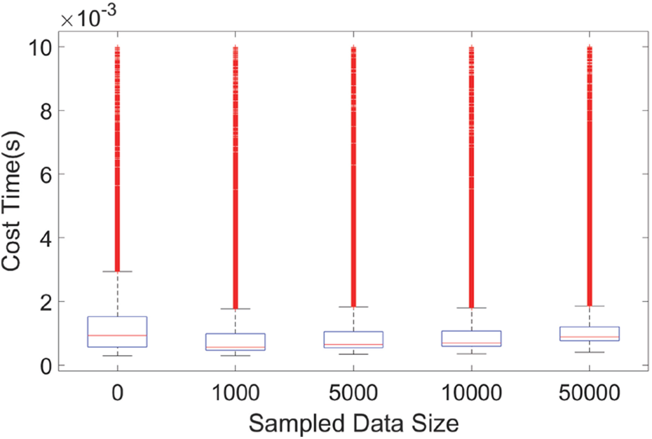
The primitive analytical and numerical IK solvers are IKfast, NR, LMA, and SQP. The speedup versions are IKfast-SP, NR-SP, LMA-SP, and SQP-SP. Between the joint limit ranges, 100,000 random configurations of the left arm are generated, and their corresponding poses are computed by forward kinematics. These IK solvers search the IK solution for the 100,000 poses. In the IKfast solver, the free joint is the sixth joint, and the initial value is zero. The initial value is zero for all joints in the three numerical solvers: NR, LMA, and SQP. The sampled data size used for the speedup method is 1000, 5000, 10,000, and 50,000 in the four speedup IK solvers: IKfast-SP, NR-SP, LMA-SP, and SQP-SP. The value of timeout is 0.01s for each IK solver. Average cost time and success rate per IK solver call are measured, and the results are shown in Tables 2 and 3. We visualize the summary statistics of the running time with a box plot, as shown in Figures 2 to 5. In Figures 2 to 5, when the sampled data size is zero, it means that the IK solvers use the zero configuration or a random joint state as the initial guess.

Table 2.

Average cost time per IK solver call (ms).

	IK solvers
Data size	IKfast-SP	NR-SP	LMA-SP	SQP-SP
1000	2.3028	0.8537	0.8238	0.9989
5000	2.2739	0.8316	0.8412	1.0888
10,000	2.0946	0.8196	0.8370	1.1192
50,000	2.5508	0.8979	0.9082	1.2912
	IKfast	NR	LMA	SQP
	14.1271	1.5437	1.1671	1.2721

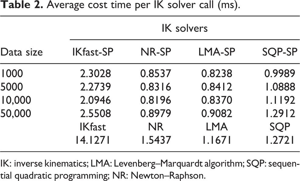
IK: inverse kinematics; LMA: Levenberg–Marquardt algorithm; SQP: sequential quadratic programming; NR: Newton–Raphson.

Table 3.

Success rate per IK solver call (%).

	IK solvers
Data size	IKfast-SP	NR-SP	LMA-SP	SQP-SP
1000	91.77	99.10	99.39	98.84
5000	92.72	99.19	99.32	98.73
10,000	94.92	99.20	99.42	98.79
50,000	94.43	99.23	99.40	98.56
	IKfast	NR	LMA	SQP
	74.53	98.92	99.28	98.96

IK: inverse kinematics; LMA: Levenberg–Marquardt algorithm; SQP: sequential quadratic programming; NR: Newton–Raphson.

Figure 2.

Running time summary of IKfast-SP. IK: inverse kinematics.

Figure 3.

Running time summary of NR-SP. NR: Newton–Raphson.

Figure 4.

Running time summary of LMA-SP. LMA: Levenberg–Marquardt algorithm.

Figure 5.

Running time summary of SQP-SP. SQP: sequential quadratic programming.

In Tables 2 and 3, the data size is the number of candidate seed states for the IK solvers. The last line is the average cost time of the primitive IK solvers in Table 2. The IKfast solver has the longest running time, up to $14.1271 ms$ . When the sampled data size is 10,000, the IKfast-SP, NR-SP, and LMA-SP solvers have the best performance. However, for the SQP-SP solver, the average cost time is the smallest when the sampled data size is 1000. In terms of the success rate, there is no significant change in the NR-SP, LMA-SP, and SQP-SP and their primitive versions. However, the IKfast-SP solver promotes the percentage compared to the IKfast.

The zero configuration is taken as the seed state for the four primitive IK solvers in the simulation. If the joint distance is far from the desired configuration for a random robot configuration, the numerical IK solvers will execute more iterations before they find the IK solutions. In addition, using the default initial guess, the NR and LMA solvers may fail, and in this case, a new joint state will be generated at random and taken as the seed state. However, the speedup method provides a closer configuration as the seed state and results in fewer iterations, as shown in Table 4. As for the IKfast solver, the initial value assigned to the free joint is not possibly suitable or is far from the theoretical value. The IKfast solver spends more time with several iterations to change the value of the free joint before solving the IKP, but in most cases, the speedup method chooses a better initial value. Due to the timeout being set to a short time, for example, $0.01 s$ , the primitive IK solvers will fail before the convergence. In Tables 2 and 4, it is obvious that the IKfast-SP, NR-SP, LMA-SP, and SQP-SP solvers are more efficient in solving the IKP than the primitive ones.

Table 4.

An IK example for performance comparison.

IK solvers	Iteration	Time (ms)	Error	J0	J1	J2	J3	J4	J5	J6
IKfast	9	3.378	7.74E−06	0.014934	−0.110798	−2.138208	2.023885	−0.120769	−0.120000	−0.209480
IKfast-SP	1	0.496	7.74E−06	−0.576637	0.490358	−2.723317	2.116051	−1.088432	−0.767574	1.357421
LMA	5	3.181	2.51E−05	0.197011	−0.502955	−1.991701	2.003437	1.043405	−0.352746	−1.699305
LMA-SP	1	0.769	3.44E−05	0.262207	−0.671714	−1.935135	1.991724	1.085539	−0.492178	−1.879615
NR	2	17.100	7.26E−07	−0.968328	−1.776231	0.044129	2.159070	−2.203004	1.342319	0.573050
NR-SP	1	2.732	1.76E−06	0.262249	−0.671822	−1.935098	1.991708	1.085634	−0.492262	−1.879798
SQP	1	3.283	1.82E−06	0.035950	−0.149763	−2.124205	2.020219	0.132647	−0.119594	−0.497306
SQP-SP	1	0.593	6.86E−07	0.263031	−0.673925	−1.934434	1.991556	1.085758	−0.493992	−1.881667

IK: inverse kinematics; LMA: Levenberg–Marquardt algorithm; SQP: sequential quadratic programming; NR: Newton–Raphson.

Conclusion

To improve analytical and numerical IK solutions, we propose a speedup method. The speedup method performs random sampling many times in the configuration space, saves those configurations that satisfy the given constraints and their corresponding pose data, and generates a database file with a designed data structure. For a desired end-effector pose, the method searches the pose data loaded into memory according to the proximity principle until the nearest pose is found. Then, it uses the corresponding joint values of the nearest pose as the initial guess.

We have three conclusions: (1) if the original IK solver is slow, significant improvements can be obtained with the speedup method; (2) if the original IK solver is fast, then the speedup method does not improve performance much and can make it worse; and (3) for the analytical method, IKfast, the speedup method can acquire better success rate. In addition, performance can potentially be improved by tuning sampled data sizes. The result in the third section verifies that the proposed method promotes the performance of the primitive IK solvers.

Our speedup method is to choose a better initial guess for four IK methods to solve the IKP of 7-DOF robots, and we do not consider the singular problem for the time being. Of course, the speedup method is applicable to modify the numerical approach²⁹ for 6-DOF robots, but research on whether it has the advantage over the closed-form methods³⁰ needs to be done in the future. In addition, we do not test whether the speedup method can be applied to parallel³¹ and hybrid robots.^32,33 Much more work should be done before the method can solve the IKP of parallel and hybrid robots.

Footnotes

Appendix 1 Declaration of conflicting interests

The author(s) declared no potential conflicts of interest with respect to the research, authorship, and/or publication of this article.

Funding

The author(s) disclosed receipt of the following financial support for the research, authorship, and/or publication of this article: This work was supported in part by the National Key Research and Development Program of China under Grant 2019YFB1310201.

ORCID iD

Shuxin Xie

References

Beeson

Ames

. TRAC-IK: an open-source library for improved solving of generic inverse kinematics. In: Proceedings of the IEEE RAS humanoids conference, Seoul, South Korea, 3–5 November 2015, pp. 928–935. DOI: 10.1109/HUMANOIDS.2015.7363472.

Mokhtari

Eisen

Ribeiro

An incremental quasi-Newton method with a local superlinear convergence rate. In: 2017 IEEE international conference on acoustics, speech and signal processing (ICASSP), New Orleans, LA, USA, 5–9 March 2017, pp. 4039–4043. DOI: 10.1109/ICASSP.2017.7952915.

Funda

Paul

. A computational analysis of screw transformations in robotics. IEEE Trans Robot Autom 1990; 6(3): 348–356.

Ayiz

Kucuk

. The kinematics of industrial robot manipulators based on the exponential rotational matrices. In: 2009 IEEE international symposium on industrial electronics, Seoul, South Korea, 5–8 July 2009, pp. 977–982. IEEE.

Giamou

Maric

Rosen

, et al. Convex iteration for distance-geometric inverse kinematics. IEEE Robot Autom Lett 2022; 7(2): 1952–1959.

Aydin

Kucuk

. Quaternion based inverse kinematics for industrial robot manipulators with Euler wrist. In: 2006 IEEE international conference on mechatronics, Budapest, Hungary, 3–5 July 2006, pp. 581–586. IEEE.

Huang

Tan

Inverse kinematics of compliant manipulator based on the immune genetic algorithm. In: 2008 fourth international conference on natural computation, volume 4, Jinan, China, 18–20 October 2008, pp. 390–394. DOI: 10.1109/ICNC.2008.631.

Dulęba

Opałka

. A comparison of Jacobian-based methods of inverse kinematics for serial robot manipulators. Int J Appl Math Comput Sci 2013; 23(2): 373–382.

Ratajczak

. Design of inverse kinematics algorithms: extended Jacobian approximation of the dynamically consistent Jacobian inverse. Arch Contr Sci 2015; 25(1): 35–50.

10.

Chiacchio

Chiaverini

Sciavicco

, et al. Closed-loop inverse kinematics schemes for constrained redundant manipulators with task space augmentation and task priority strategy. Int J Robot Res 1991; 10(4): 410–425.

11.

Zghal

Dubey

Euler

Efficient gradient projection optimization for manipulators with multiple degrees of redundancy. In: Proceedings, IEEE international conference on robotics and automation, volume 2, Cincinnati, OH, USA, 13–18 May 1990, pp. 1006–1011. DOI: 10.1109/ROBOT.1990.126123.

12.

Buss

. Introduction to inverse kinematics with Jacobian transpose, pseudoinverse and damped least squares methods. IEEE J Robot Automat 2004; 17(1–19): 16.

13.

Chan

Dubey

. A weighted least-norm solution based scheme for avoiding joint limits for redundant joint manipulators. IEEE Trans Robot Automat 1995; 11(2): 286–292.

14.

Dimovski

Trompeska

Samak

, et al. Algorithmic approach to geometric solution of generalized Paden–Kahan subproblem and its extension. Int J Adv Robot Syst 2018; 15(1): 1729881418755157.

15.

Bae

JH.

Analytic inverse kinematics considering the joint constraints and self-collision for redundant 7DOF manipulator. In: 2017 first IEEE international conference on robotic computing (IRC), Taichung, Taiwan, 10–12 April 2017, pp. 123–128. DOI: 10.1109/IRC.2017.46.

16.

Gong

Zhang

. Analytical inverse kinematics and self-motion application for 7-DOF redundant manipulator. IEEE Access 2019; 7: 18662–18674.

17.

Hemami

. A more general closed-form solution to the inverse kinematics of mechanical arms. Adv Robot 1987; 2(4): 315–325.

18.

Diankov

. Automated construction of robotic manipulation programs. PhD Thesis, Carnegie Mellon University, 2010.

19.

Manocha

Zhu

. A fast algorithm and system for the inverse kinematics of general serial manipulators. In: Proceedings of the 1994 IEEE international conference on robotics and automation, San Diego, CA, USA, 8–13 May 1994, pp. 3348–3353. IEEE.

20.

Manocha

Canny

JF.

Real time inverse kinematics for general 6R manipulators. In: Proceedings 1992 IEEE international conference on robotics and automation, volume 1, Nice, France, 12–14 May 1992, pp. 383–389. DOI: 10.1109/ROBOT.1992.220309.

21.

Sugihara

. Solvability-unconcerned inverse kinematics based on Levenberg-Marquardt method with robust damping. In: 2009 9th IEEE-RAS international conference on humanoid robots, Paris, France, 7–10 December 2009, pp. 555–560. IEEE.

22.

Wilamowski

. Improved computation for Levenberg–Marquardt training. IEEE Trans Neural Networks 2010; 21(6): 930–937.

23.

Luh

Walker

Paul

. Resolved-acceleration control of mechanical manipulators. IEEE Trans Autom Control 1980; 25(3): 468–474.

24.

Nakamura

Hanafusa

. Inverse kinematic solutions with singularity robustness for robot manipulator control. J Dyn Syst Meas Contr 1986; 108(3): 163–171.

25.

Badreddine

Vandewalle

Meyers

. Sequential quadratic programming (SQP) for optimal control in direct numerical simulation of turbulent flow. J Comput Phys 2014; 256: 1–16.

26.

Kou

Dai

. A modified self-scaling memoryless Broyden–Fletcher–Goldfarb–Shanno method for unconstrained optimization. J Optim Theory Appl 2015; 165(1): 209–224.

27.

Kraft

. A software package for sequential quadratic programming. Technical Report 88-28, Institutfür Dynamik der Flugsysteme, Obersfaffeuhofen, Germany, 1988.

28.

Craig

. Introduction to robotics: mechanics and control. Upper Saddle River, NJ: Pearson Prentice Hall, 2005.

29.

Hayat

Sadanand

ROM

Saha

. Robot manipulation through inverse kinematics. In: Proceedings of the 2015 conference on advances in robotics, Goa, India, July 2015, pp.1–6. DOI: 10.1145/2783449.2783497.

30.

Tian

Zhan

. An analytical inverse kinematics solution with joint limits avoidance of 7-DOF anthropomorphic manipulators without offset. J Franklin Inst 2021; 358(2): 1252–1272.

31.

Kucuk

. Simulation and design tool for performance analysis of planar parallel manipulators. Simulation 2012; 88(5): 542–556.

32.

Tanev

. Kinematics of a hybrid (parallel–serial) robot manipulator. Mech Mach Theory 2000; 35(9): 1183–1196.

33.

Kucuk

Gungor

. Inverse kinematics solution of a new hybrid robot manipulator proposed for medical purposes. In: 2016 medical technologies national congress (TIPTEKNO), Antalya, Turkey, 27–29 October 2016, pp. 1–4. IEEE.

A speedup method for solving the inverse kinematics problem of robotic manipulators

Abstract

Keywords

Introduction

Methods

IKfast approach

Newton–Raphson method

Levenberg–Marquardt algorithm

Sequential quadratic programming method

Speedup method based on sampled data

Results and discussion

Conclusion

Footnotes

Appendix 1

Declaration of conflicting interests

Funding

ORCID iD

References