Research on cooperative optimization of multiphase pump impeller and diffuser based on adaptive refined response surface method

Abstract

Multiphase pumps play an important role in the exploitation of natural gas hydrate. Compared with ordinary pumps, they can handle fluids with higher gas volume fraction (GVF). Therefore, it is important to improve the performance of the pump under high GVF. A model pump is designed based on the design theory of axial flow pump and centrifugal pump inducer. The hydraulic performance of the model pump is verified by numerical simulation and experiment. The Sparse Grid method is applied to the design of experiment (DOE), and three different adaptive refined response surface methods (RSM) are applied to the build the approximate model. Refinement points and verification points are used to improve and verify the precision of the response surface, respectively. The model with high precision and high computational efficiency is obtained through comparison and analysis. The multi-objective optimization of the optimal response surface model is carried out by MOGA (Multi-Objective Genetic Algorithm) method. The pressure increment of the optimized model is increased by 38 kPa. The efficiency is significantly improved under large mass flow conditions. The hydraulic performance of the optimized model is compared with that of the basic model. And the reasons that affect the performance of the multiphase pump are analyzed.

Introduction

Natural gas hydrate is a new energy with high combustion value and low pollution formed by water and natural gas under specific temperature and pressure conditions. There is abundant natural gas hydrate resource all over the world. Natural gas hydrate is considered as another high-efficiency alternative energy with mining potential after shale gas, tight gas, and coalbed methane. A turbine pump device for exploiting natural gas hydrate is proposed in Figure 1. The fluid impacts the turbine to provide power and drive the main shaft to rotate. The axial flow pump, connected with the turbine through the coupling, drives the impeller of the pump to rotate to achieve the purpose of pumping natural gas hydrate. Due to the particularity of the medium, the traditional axial flow pump cannot achieve the purpose of gas-liquid mixed transportation.

Figure 1.

Turbine pumping device.

Multiphase pump technology was first proposed by Dal Porto. ¹ Years of field application have proved that this technology can transport gas-liquid mixed fluid well. Therefore, a turbine pump device with a multistage turbine and multistage multiphase pump as the main power part can achieve the purpose of exploiting natural gas hydrate.

The impeller and diffuser are the most important parts of the multiphase pump. To improve the performance of the multiphase pump, some scholars have studied the design method of the impeller. Controllable blade angle method, ² numerical solution of meridian flow net method, ³ and inverse design method ⁴ are proposed for the design of multiphase pumps. Liu et al., ⁵ Suh et al., ⁶ and Zhang et al. ⁷ studied the interphase force in the fluid of the multiphase pump, improved the precision of numerical simulation, and the results were closer to the experimental. Shi et al. ⁸ analyzed the energy conversion characteristics of multiphase pump blades, and the influence law of the change of blade wrap angle on the energy transfer performance of multiphase pump was obtained. The influences of viscosity, flow rate, and blade height on the distribution of turbulence kinetic energy are analyzed by Liu et al. ⁹ Characteristics of partial differential equations are employed to reveal the influence of viscosity, and a theoretical model has been established to predict the influence of flow rate. Sano et al. ¹⁰ conducted an experimental study on the flow characteristics inside the multiphase pump, obtained the pressure distribution, and blade load distribution of the impeller under different GVF. Unstable flow phenomenon was found under the condition of small flow. Shi ¹¹ used numerical simulation and experimental research to reveal the influence of inlet GVF on tip clearance flow characteristics, and the results showed that the gas was mainly distributed near impeller inlet pressure side, tip clearance, and suction side. Shi and Zhu ¹² puts forward a stage-by-stage design method to improve the pressure increment of multiphase pump, and the pressure increment of the pump is improved.

In the aspect of optimization, Han et al. ¹³ analyzed the influence of different thickening ratio coefficients on the transport characteristics of the multiphase pump and obtained the airfoil thickening model with low gas aggregation. The improved pump head coefficient was 5.8% higher than the basic pump, and the efficiency increased by 3.1%. Shi et al. ¹⁴ proposed a blade structure with cracks, which effectively improved the performance of a multiphase pump with high GVF. Shi et al. ¹⁵ used orthogonal test and CFD technology to optimize the model pump. After optimization, the pump head and efficiency were increased by 2.81m and 5.6% respectively. Liu et al. ¹⁶ proposed a new method to predict and optimize the performance of a multiphase pump based on Oseen vortex theory. The established theoretical model could predict the velocity moment of the downstream flow field of a diffuser, and apply it to angle optimization of the inlet blade of the impeller of the next stage. Kim et al., ¹⁷ Hao et al., ¹⁸ and Zhang et al. ¹⁹ optimized the impeller of the multiphase pump and obtained a better impeller model with improved head and efficiency. Suh et al. ²⁰ optimized the angle of impeller and diffuser of a multiphase pump with a single objective respectively. The hydraulic performance of the pump has been significantly improved. A design method of controllable velocity moment in combination of singularity method is proposed for multiphase pump by Xiao and Tan, ²¹ the pressurization and efficiency of the pump have been improved. According to the direct search optimization technology and complex method, Yang et al. ²² developed a design optimization program coupled with the mathematical model to optimize the design of multiphase pump. The efficiency of the pump is improved, and the relationship between GVF and cylinder structure is obtained. Kim et al. ²³ designed the multi-phase pump using multi-objective optimization design technology, established the optimization model by response surface method, and analyzed the influence of GVF on the multi-phase flow performance of the optimization model.

On the one hand, some scholars have optimized the impeller of the multiphase pump, and some have optimized the impeller and diffuser separately. However, the performance of the impeller and diffuser in a multiphase pump is mutually affected. Optimizing one alone may not achieve the expected result. On the other hand, most scholars directly use the data generated by experimental design to construct response surfaces. The accuracy of the response surface is closely related to the number of sampling points. This paper uses the fewest points to design the experiment and build the initial response surface model. Then use different adaptive refined methods to improve the precision of the response surface. Based on this method, the impeller and diffuser of the multiphase pump are co-optimized. Finally, the performance of the multi-phase pump before and after optimization is compared and analyzed, which proves that the method is effective.

The chapters of this paper are arranged as follows. In chapter 2, the optimization theory is introduced briefly. In Chapter 3, a model pump was designed and the performance curves under different working conditions are obtained by numerical simulation. The results are verified by experiment. In Chapter 4, we introduce the whole optimization process and verify the optimization results. The flow field characteristics before and after optimization are compared and analyzed, and the reasons for the performance change of the multiphase pump are obtained in Chapter 5. Finally, we summarize the work of this paper.

Methods and theories

Sparse grid model

Sparse Grid theory was first used to solve high-dimensional partial differential equations, now it is also widely used in approximate model construction and other fields.^24–26 The biggest advantage is that it can alleviate the exponential dependence of the number of sample points on the dimension. The number of sample points is greatly reduced, and the precision of the model can be guaranteed when dealing with high-dimensional models. When solving the d-dimensional problem, N points need to be collected in each dimension, a total of $M(N^d)$ points need to be collected. The Sparse Grid method only needs to collect $M(N(\log N{)}^{d-1})$ points to meet the precision requirements.

Sample space

According to the L1-norm principle, the sample point space with precision level n is defined as follows.

$${\mathit{V}}_{\mathit{n}}^{(1)}:=\sum _{{\mathit{l}}_1=1}^{\mathit{n}}\dots \sum _{{\mathit{l}}_{\mathit{d}}=1}^{\mathit{n}}{\mathit{W}}_{({\mathbf{l}}_1,{\mathbf{l}}_2,\dots ,l_{\mathbf{d}})}\mathbf{=}\underset{{\left|\underset{-}{\mathit{l}}\right|}_1\le \mathit{n}+\mathit{d}-1}{\oplus }{\mathit{W}}_{\underset{-}{\mathit{l}}}$$

(1)

The number of degrees of freedom reduction in the sample point space is as follows.

$$\left|{\hat{\mathit{V}}}_{\mathit{n}}\right|=\sum _{\mathit{i}=0}^{\mathit{n}-1}{2}^{\mathit{i}}\left(\begin{array}{c}\mathit{d}-1+\mathit{i}\hfill \\ \multicolumn{1}{c}{\mathit{d}-1}\end{array}\right)=\mathit{O}({\mathit{h}}_{\mathit{n}}^{-1}{\left|\mathbf{lo}{\mathbf{g}}_2{\mathit{h}}_{\mathit{n}}\right|}^{\mathit{d}-1})$$

(2)

According to equations (1) and (2), each subspace and sample point space of the two-dimensional problem is shown in Figure 2. ²⁴

Figure 2.

Subspace and combined sample point space of Sparse Grids.

Approximate model based on Sparse Grid theory

The solution formula U(f) for solving a one-dimensional problem with the Sparse Grid model is:

$$\mathit{U}(\mathit{f})=\sum _{\mathit{j}=1}^{{\mathit{m}}_{\mathit{i}}}{\mathit{a}}_{\mathit{j}}^{\mathit{i}}\mathit{f}({\mathit{x}}_{\mathit{j}}^{\mathit{i}})$$

(3)

Where: i is the precision level of the model, i∈n; j is the sample point, j  = 1, 2, …, m_i , m_i is the number of sample points; Basis function ${\mathit{a}}_{\mathit{j}}^{\mathit{i}}\in \mathit{C}\mathbf{(}\mathbf{[}-1,1\mathbf{]}\mathbf{)}$ ; Sampling point ${\mathit{x}}_{\mathit{j}}^{\mathit{i}}\in [-1,1]$ .

The design variable x is normalized by segments. When solving multidimensional problems, the Smlolyak algorithm ²⁷ and tensor product formula are used to transform the solution formula of the model. The approximate model solution formula is transformed into:

$$\begin{array}{c}({\mathit{U}}^{{\mathit{i}}_1}\otimes \dots \otimes {\mathit{U}}^{{\mathit{i}}_{\mathit{d}}})\left(\mathit{f}\right)\hfill \\ =\sum _{{\mathit{j}}_1}^{{\mathit{m}}_{{\mathit{i}}_1}}\sum _{{\mathit{j}}_{\mathit{d}}=1}^{{\mathit{m}}_{{\mathit{i}}_{\mathit{d}}}}\mathit{f}({\mathit{x}}_{{\mathit{j}}_1}^{{\mathit{i}}_1},\dots ,{\mathit{x}}_{\mathit{jd}}^{\mathit{id}})•({\mathit{a}}_{{\mathit{j}}_1}^{{\mathit{i}}_1}\otimes \dots \otimes {\mathit{a}}_{{\mathit{j}}_{\mathit{d}}}^{{\mathit{i}}_{\mathit{d}}})\hfill \end{array}$$

(4)

Where d is the dimension of the model, i₁, i₂,…, i_d is the precision level of each dimension of the model. j_d is the sample point of each dimension, m_i1, m_i2,…, m_id are the sample points of each dimension.

Another advantage of using the Sparse Grid method to solve the approximate model is the priority fitting precision brought by its hierarchical basis function. The current fitting precision is:

$${\mathit{w}}_{\mathit{j}}^{\mathit{i}}={\mathit{f}(x}_{\mathit{j}}^{\mathit{i}})-{\mathit{U}}^{\mathit{i}-1}{(\mathit{f})(x}_{\mathit{j}}^{\mathit{i}})$$

(5)

When the precision ${\mathit{w}}_{\mathit{j}}^{\mathit{i}}$ reaches the standard, the generation of sample points and approximate models in the sample space will stop automatically.

Kriging model

The Kriging method is widely used in optimization research.^28,29 It is a multi-dimensional interpolation technology, considering both global and local common influencing factors. Kriging response surface passes through all design points, so it is suitable for highly nonlinear complex engineering optimization problems. It can solve both isotropic and anisotropic problems, and avoid the problems of poor fitting degree and local optimization of primary response surface and secondary response surface.

Based on the Kriging method, its output parameters are equal to the global design space plus partial deviation. Its expression is:

$$\mathit{y}(x)=\mathbf{F}(\beta ,\mathit{x})+\mathbf{z}(\mathbf{x})={\mathit{f}}^{\mathit{T}}(\mathbf{x})\beta +\mathit{z}(\mathbf{x})$$

(6)

Where β is the regression coefficient of the basis function. f(x) is the polynomial function of variable x, representing the global model of design space. z(x) is a Gaussian random function with a mean of 0 and a variance of ${\sigma }^2$ .The expectation and covariance are E(Z(x)) = 0.

$$\mathit{Cov}[\mathit{Z}(x),Z(u)]={\sigma }^2\mathit{R}\mathbf{(}\mathbf{x}\mathbf{,}\mathbf{u}\mathbf{,}\theta \mathbf{)}$$

(7)

Where ${\sigma }^2$ is the variance. θ is the parameter of the correlation function, which is used to measure the attenuation degree of the correlation between sample point t and sample point u with the increase of the distance between two points. The smaller the correlation is, the smoother the generated response surface is.

R(x, u, θ) is the variogram between points t and u, and its general form is:

$$\mathit{R}(\mathbf{x}\mathbf{,}\mathbf{u}\mathbf{,}\theta )=\underset{\mathit{i}}{\overset{\mathit{n}}{\Pi }}{\mathit{R}}_{\mathit{j}}\mathbf{(}{\mathbf{d}}_{\mathit{j}}\mathbf{)}$$

(8)

Where R_j(d_j) is the kernel function of the variogram, usually in the form of a Gaussian function. n is the dimension of the variogram, θ is the parameter of the correlation function, and d is the distance between data points.

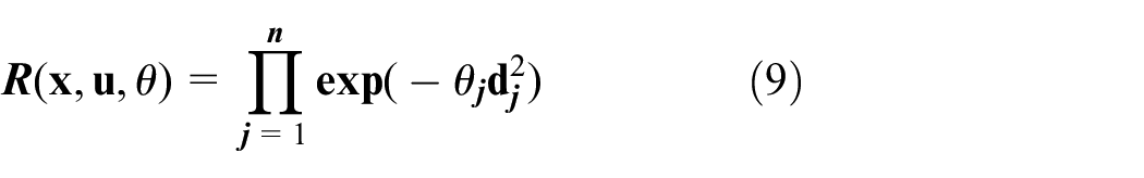
The form of the variogram is as follows.

$$\mathit{R}\mathbf{(}\mathbf{x}\mathbf{,}\mathbf{u}\mathbf{,}\theta \mathbf{)}=\underset{\mathit{j}=1}{\overset{\mathit{n}}{\Pi }}\mathbf{exp}\mathbf{(}-{\theta }_{\mathit{j}}{\mathbf{d}}_{\mathit{j}}^2\mathbf{)}$$

(9)

The design points of DOE are used to form a correlation matrix.

$$\left(\begin{array}{ccc}\mathit{R}\mathbf{(}{\mathbf{x}}_1,{\mathbf{x}}_1\mathbf{)}\hfill & \dots \hfill & \mathit{R}\mathbf{(}{\mathbf{x}}_1,{\mathbf{x}}_{\mathit{w}}\mathbf{)}\hfill \\ \multicolumn{1}{c}{⋮}& \ddots \hfill & ⋮\hfill \\ \multicolumn{1}{c}{\mathit{R}\mathbf{(}{\mathbf{x}}_{\mathit{w}},{\mathbf{x}}_1\mathbf{)}}& \cdots \hfill & \mathit{R}\mathbf{(}{\mathit{x}}_{\mathbf{w}},{\mathit{x}}_{\mathit{w}}\mathbf{)}\hfill \end{array}\right)$$

(10)

Where w is the total number of data points, and the polynomial parameters of the Kriging model are obtained by using the weighted least square method:

$${\beta }^{\wedge }=\mathbf{(}{\mathbf{x}}^{\mathit{T}}{\mathbf{R}}^{-1}{\mathbf{x}\mathbf{)}}^{-1}{\mathit{x}}^{\mathit{T}}{\mathit{R}}^{-1}\mathit{Y}$$

(11)

Where x is the coefficient matrix composed of experimental design points; Y is the response value corresponding to the design point in the experimental design. Similarly, the estimate of variance is:

$${\sigma }^2=\mathbf{(}\mathbf{Y}\mathbf{-}\mathbf{x}\beta {\mathbf{)}}^{\mathit{T}}{\mathit{R}}^{-1}\mathbf{(}\mathbf{Y}-\mathbf{x}\beta \mathbf{)}$$

(12)

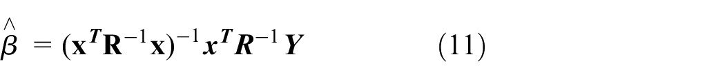
Finally, the basis function coefficients β and Gaussian random variance are determined by the sample points and correlation functions designed in the experiment.

$$\hat{\mathit{y}}(\mathit{x})=\stackrel{\wedge }{{\beta }^{\mathit{T}}}\mathit{f}:\mathbf{(}\mathbf{x}\mathbf{)}+\mathbf{r}\mathbf{(}\mathbf{x}\mathbf{)}{\mathbf{R}}^{-1}\mathbf{(}\mathbf{y}-\mathbf{F}{\beta }^{\wedge })$$

(13)

The Kriging response surface is generated to predict the value of any design point.

$$\hat{\mathit{y}}(\mathit{x})=\stackrel{\wedge }{{\beta }^{\mathit{T}}}\mathit{f}\mathbf{(}\mathbf{x}\mathbf{)}+{\mathbf{r}}^{\mathit{T}}\mathbf{(}\mathbf{x}\mathbf{)}{\mathbf{R}}^{-1}\mathbf{(}\mathbf{y}-\mathbf{F}{\beta }^{\wedge })$$

(14)

R is the correlation matrix, and r^T(x) is the vector of the relationship between the unknown and the known point.

Neural network model

A neural network^30,31 is a mathematical technique based on the natural neural network in the human brain. To interpolate a function, a network with three levels (input, hidden, and output) is built and the connections between them are weighted, as shown in Figure 3. Each arrow is associated with a weight.

Figure 3.

Structure diagram of neural network.

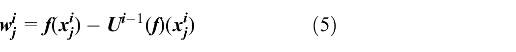
Each ring is called a cell (like a neuron). If the inputs are x_i, the hidden level contains function g_j(x_i). The output solution is:

$${\mathit{f}}_{\mathit{k}}\mathbf{(}{\mathbf{x}}_{\mathit{i}}\mathbf{)}=\mathbf{K}[\sum {\mathit{w}}_{\mathit{jk}}{\mathit{g}}_{\mathit{j}}\mathbf{(}{\mathbf{x}}_{\mathit{i}}\mathbf{)}]$$

(15)

Where K is a predefined function, such as the hyperbolic tangent or an exponential based function, to obtain something similar to the binary behavior of the electrical brain signal (like a step function). The function is continuous and differentiable.

The weight functions w _jk are issued from an algorithm that minimizes (as the least squares method) the distance between the interpolation and the known values (design points). This is called learning. The error is checked at each iteration with the design points that are not used for learning. Learning design points need to be separated from error-checking design points. The error decreases and then increases when the interpolation order is too high. The minimization algorithm is stopped when the error is the lowest.

Base model and numerical simulation

Base model design

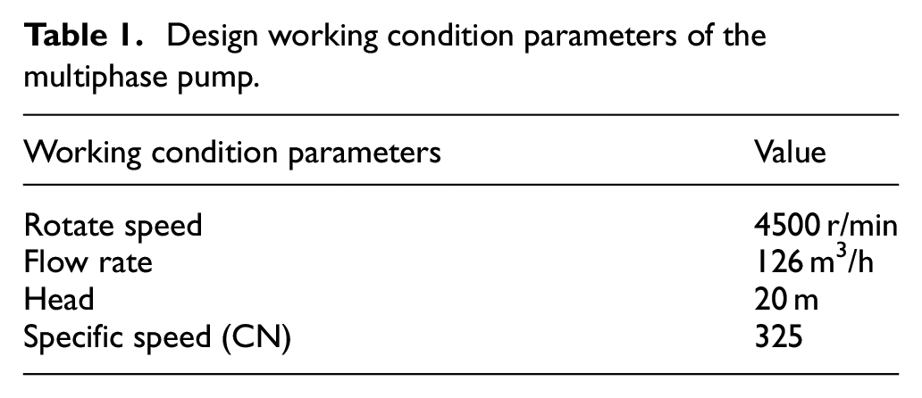
In this paper, a model pump is designed according to the working condition parameters in Table 1. Firstly, the head coefficient and the parameters such as impeller shroud diameter are determined based on the working condition. The structural parameters of the impeller are calculated according to the design theory of axial flow pump and guide vane of centrifugal pump diffuser. The inlet shroud flow angle is determined according to the inlet speed and the circumferential speed of the shroud. Inlet and outlet angles of the blade at the shroud and hub are obtained by the principle of equal radial lead of the blade, as shown in formula (16).

Table 1.

Design working condition parameters of the multiphase pump.

Working condition parameters	Value
Rotate speed	4500 r/min
Flow rate	126 m 3 /h
Head	20 m
Specific speed (CN)	325

$$\mathit{Const}=\mathit{rtan}\alpha$$

(16)

Where r is the radius of the blade, α means the flow angle.

791 special-shaped thickening is used for blade profile. The design method of the diffuser is similar to that of the impeller. The basic parameters of the designed model pump are shown in Table 2, and the final model pump and details are shown in Figure 4.

Table 2.

Blade profile parameters of the multiphase pump.

	Shape parameters	Value	Unit
Impeller	Shroud diameter (a1)	137	mm
	Hub inlet diameter (a2)	96	mm
	Hub outlet diameter (a3)	108	mm
	Hub length (a4)	58	mm
	Number of impellers (a5)	3
	Hub inlet flow angle (a6)	16.1	°
	Hub outlet flow angle (a7)	18	°
	Wrap angle (a8)	173	°
	Tip clearance (a9)	0.5	mm
Diffuser	Hub inlet flow angle (b1)	41.7	°
	Hub outlet flow angle (b2)	90	°
	Hub length (b3)	58	mm
	Number of diffusers (b4)	11
	Wrap angle (b5)	32.7	°
	Clearance between impeller and diffuser (c1)	2	mm

Figure 4.

Model diagram of single-stage multiphase pump: (a) 3D model diagram, (b) dimensions of impeller and diffuser, (c) hub inlet and outlet flow angle of impeller and diffuser, and (d) wrap angle of impeller and diffuser.

Numerical simulation

Boundary conditions

Speed condition is used at the inlet. Opening condition is used at the outlet. In actual working conditions, there will be backflow at the outlet of the pump, and the backflow will be more obvious especially in the case of a small flow rate. So we choose the opening outlet to represent the generation of backflow, which follows the flow law. The boundary conditions are shown in Table 3. The Euler-Euler model is used to simulate two-phase flow. Bubbles with a diameter of 0.1 mm are used in the gas phase, and water is used in the liquid phase. The gas phase is simulated by the zero equation model, and the liquid phase is simulated by SST (Shear Stress Transfer) model. The frozen rotor technology is used to simulate the dynamic and static interface.^8,20 Due to the existence of the gap at the top of the impeller, the boundary of the counter-rotating wall is used to simulate the outer shroud of the impeller. The convection term and turbulence term are solved by high-resolution, and the convergence precision is set to 10-5. The changes of inlet and outlet flow balance, efficiency, and pressure increment are monitored during the calculation. When the flow balance is less than 0.1%, the calculation is considered to meet the convergence precision requirements.

Table 3.

Settings of boundaries.

Boundaries	Settings and value
Reference pressure	All zone	1 atm
Inlet	Normal speed	4.53 m/s
Outlet	Opening (relative pressure)	1 atm
Impeller rotating speed	4500 rpm/min
Rotor wall (impeller shroud)	Counter rotating wall
Other wall	No-slip wall
Rotor-stator interface	Frozen-rotor

Grid independence verification

The grid independence analysis of the base model is carried out under the water condition. The grid adopts an adaptive structured grid and near-wall grid encryption, which can accurately simulate the actual working conditions of the pump. Literature ³² pointed out that if the y+ value is less than 100, the thickness of the first layer of mesh can meet the requirements of the wall function. Therefore, we choose the grid y+ value to be 10, which can better meet the calculation requirements.

Grid independence verification is shown in Table 4. With the increase in the number of grids, the pressure increment of the multiphase pump does not change significantly. When the total number of grids reached 1.96 and 2.53 million, the efficiency change was only 0.011%. Therefore, the subsequent simulations in this paper use 1.96 million grids. Figure 5 shows the final grid diagram used for the following calculation.

Table 4.

Grid independence verification.

Total number of grids cells	Inlet	Impeller	Diffuser	Outlet	Pressure increment (MPa)	Efficiency (%)
642,923	99,268	363,111	146,328	34,216	0.16923	67.356
873,988	117,312	452,256	255,812	48,608	0.16965	67.681
1,499,180	200,880	835,124	397,656	65,520	0.17001	67.699
1,960,997	232,050	1,016,627	619,080	93,240	0.17094	68.012
2,536,632	265,200	1,236,168	914,304	120,960	0.17006	68.023

Figure 5.

Grid diagram of multiphase pump.

Base model numerical simulation

Figure 6 shows the pressure increment and efficiency of the model pump with Q (mass flow rate at design point). The pressure increment curve presents an obvious hump trend, and the efficiency curve first increases and then decreases, which meets the design standard of the axial flow pump. The curve shows that the pressure increment of the model pump at the design point under the water condition is 164 kPa, and the efficiency is 68.02%.

Figure 6.

Model pump performance curve under the water condition.

Figure 7 shows the performance curve of the model pump with GVF ranging from 10% to 30%. As the GVF increases, the pressure increment and efficiency gradually decrease. When the GVF is 30%, the pressure increment at the design point is 114 kPa. There is a big difference from the corresponding pressure increment required in the actual working condition, which cannot meet the engineering demand. Therefore, the blade structure needs to be optimized to improve the pressure increment. The change of blade structure will cause the change of efficiency at the same time, which is also a performance we need to pay special attention to. Therefore, this paper chooses to optimize both pressurization and efficiency.

Figure 7.

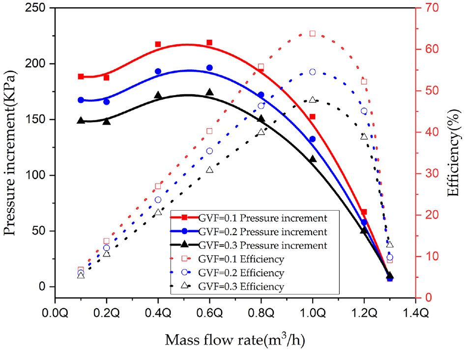
Model pump performance curve under the multiphase condition.

Validation of numerical analysis for base model

In order to verify the accuracy of numerical simulation, we carried out experimental research on turbine pumping device. Figure 8(a) shows the layout of the experiment, Figure 8(b) is the structural diagram, and Figure 8(c) is the diagram of the experiment site layout. The turbine inlet provides constant power to ensure constant shaft speed. The performance curve of the pump is obtained by adjusting the opening of the pump outlet valve. Different from the numerical simulation, the experiment is the overall test of the tool, rather than the test of a single stage of blades. The overall test included three stages of impellers of pumps used in series. The numerical simulation does not consider the use of three stages in series, but only one stage of blade.

Figure 8.

(a) Layout of the experiment. (b) Structural diagram of turbine pumping device. (1) Compression joint. (2) Fastening nut. (3) Multiphase pump. (4) Outer pipe. (5) Bearing. (6) Bridge type channel, connecting shaft and seal assembly. (7) turbine. (8) Bearing. (9) Load transfer unit. (c). Diagram of the experiment site layout. (1) Power fluid outlet. (2) Pump inlet. (3) Turbine pumping device. (4) Pressure gauge. (5) Power fluid inlet. (6) Control panel. (7) Power fluid outlet pipe. (8) Pump suction pipe. (9) Pump outlet pipe. (10) Flow meter. (11) valve. (d) Model pump performance curve of CFD and Experiment.

Figure 8(d) shows the comparison of numerical simulation and experiment data under different flow rates. Under the condition of design flow Q, the pressure increment obtained from the experiment is 402 kPa, while the numerical simulation result is 164 kPa. The numerical simulation uses a single stage blade and does not consider the energy loss caused by channel change and gap leakage in the whole machine experiment. Therefore, the results obtained in the whole machine experiment with three stages of blades will be smaller than expected. Figure 8(d) also shows that the change trend of the performance curve obtained from the experiment is similar to that of the numerical simulation. Therefore, we can consider the accuracy of numerical simulation.

Optimization

There are many kinds of optimization methods, which are generally divided into direct optimization and optimization based on approximate models. Among them, response surface model optimization is convenient and fast, and it has become the first choice of most engineering problems. Compared with the traditional response surface method, the adaptive response surface method will adaptively generate the refinement points of the response surface according to the calculation model and it has a higher level of precision. The Sparse Grid method is used to construct the experimental design in this chapter. Three different adaptive refined response surface methods, including the Sparse Grid, Kriging, and Neural Network, are used to build the approximate model. The advantages and disadvantages of the three methods are evaluated in terms of calculation efficiency, calculation precision, and goodness of fit. Finally, the optimal response surface model is optimized by the MOGA method, and the optimization results are verified by the numerical method.

Design of experiment (DOE)

Parameter selection

In the structural parameters of the impeller and diffuser, the outer diameter and axial length of the impeller are fixed due to the requirement of engineering application. In the screening of optimal parameters of multiphase pump, Kim et al. ¹⁷ used the 2K factorial design method to screen the impeller parameters, and finally concluded that the hub inlet angle and shroud outlet angle had a great impact on the performance. Zhang et al. ¹⁹ briefly introduces the relationship between the structural parameters of impeller, and takes the blade inlet angle, outlet angle and wrap angle as the optimization objectives. Suh ²⁰ introduces the interaction relationship between blade geometric parameters, and finally determines that the installation angles of impeller shroud inlet and outlet angle, and the shroud and hub inlet angle of diffuser are taken as the optimization objectives. According to the principle of equal radial lead of the blade, when we know one of the shroud or hub inlet angles, we can find the other. So is the outlet angle of the impeller. Literature ³³ proposed that the change of impeller wrap angle has a large influence on the performance of the pump. Considering that the outlet flow angle of the diffuser is 90°, which is a convention in the diffuser design process, the inlet flow angle of the shroud is selected as the design variable of the diffuser design parameters. So we finally determined four design variables, Shroud inlet angle (P1), Shroud outlet angle (P2), Wrap angle of impeller (P3), and Shroud inlet angle of diffuser (P4). The value range of each parameter of the multiphase pump is shown in Table 5.

Table 5.

Value range of experimental design variables.

	Shape parameters	Expression	Lower Bound	Upper Bound	Unit
Impeller	Shroud inlet angle	P1 $\left(\mathbf{arctan}\left(\frac{{\mathit{a}}_2\mathbf{tan}{\mathbf{a}}_6}{{\mathit{a}}_1}\right)\right)$	13	19	°
	Shroud outlet angle	P2 $\left(\mathbf{arctan}\left(\frac{{\mathit{a}}_3\mathbf{tan}{\mathit{a}}_7}{{\mathit{a}}_1}\right)\right)$	15	21
	Wrap angle	P3 (a8)	155	195
Diffuser	Shroud inlet angle	P4 $\left(\mathbf{arctan}\left(\frac{{\mathit{a}}_3\mathbf{tan}{\mathit{b}}_1}{{\mathit{a}}_1}\right)\right)$	39	45

Implementation of DOE

The Sparse Grid method is an adaptive algorithm based on a hierarchy of grids. The DOE type Sparse Grid Initialization generates a DOE matrix containing all the design points for the smallest required grid: the level 0 (the point at the current values) plus the level 1 (two points per input parameters). Sparse grid experimental design can realize the construction of experimental design with fewer points under the premise of ensuring that the test points are distributed as evenly as possible in the design space. Compared with CCD (central composite design) method and the Latin Hypercube method, the calculation is less and the efficiency is high.

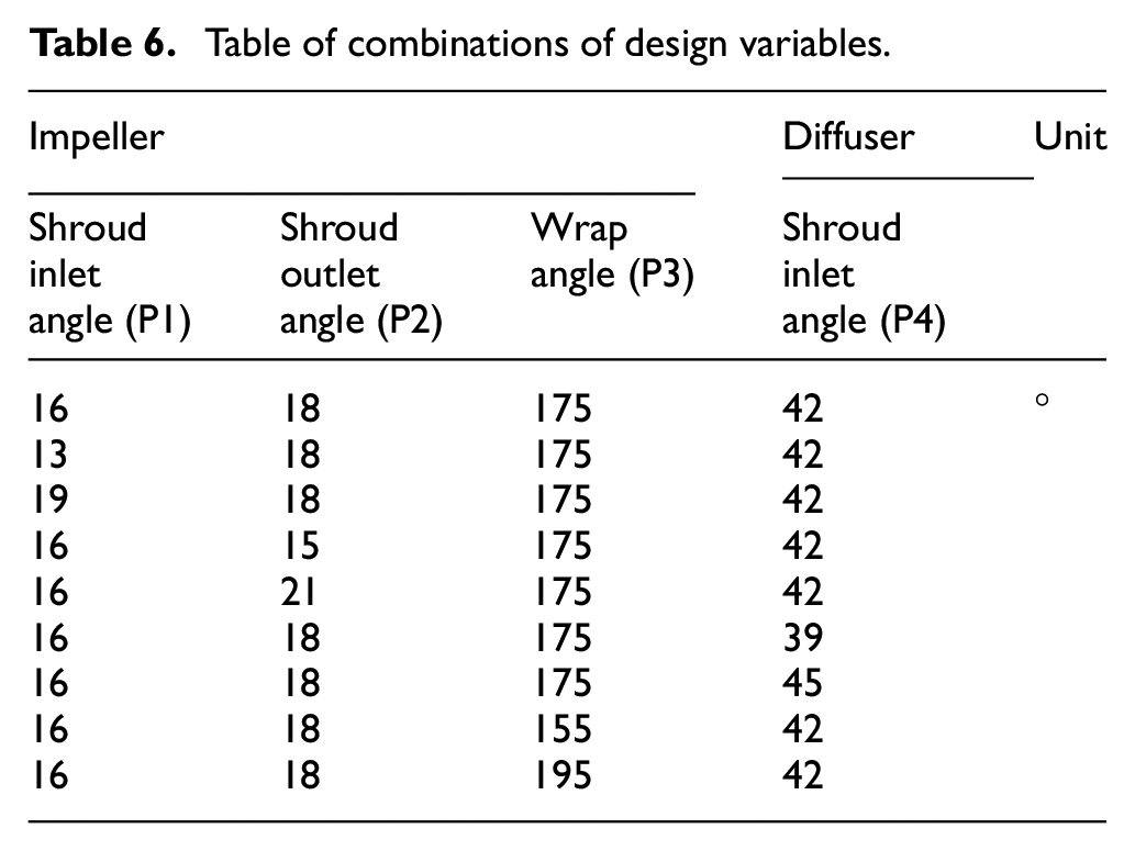
The corresponding experimental design data points are generated based on the model pump using the Sparse Grid method. Figure 9 shows the combination relationship between the generated design points. The horizontal axis represents four different design variables and the vertical axis represents the value range of four design variables. The upper right side of the figure shows that a total of nine sets of data were generated in the experimental design of Sparse Grid initialization. It can be concluded from the figure that the values of the four parameters are taken uniformly selected according to their value range, and the combination of parameters is also uniform. The values of the variables of the experimental design are given in Table 6.

Figure 9.

Parameters parallel chart.

Table 6.

Table of combinations of design variables.

Impeller			Diffuser	Unit
Shroud inlet angle (P1)	Shroud outlet angle (P2)	Wrap angle (P3)	Shroud inlet angle (P4)
16	18	175	42	°
13	18	175	42
19	18	175	42
16	15	175	42
16	21	175	42
16	18	175	39
16	18	175	45
16	18	155	42
16	18	195	42

Adaptive refined response surface method

The amount of experimental data generated based on Sparse Grid initialization is small. If these points are used directly to construct the response surface, the fitting precision is low. Therefore, it is necessary to interpolate and refine the experimental data. Three different adaptive refined response surface methods are used to improve the precision of the original response surface, as shown below.

Sparse Grid method

Based on the experimental design, a new level is established in the corresponding direction to further refine the Sparse Grid response surface. Repeat this process until the response surface reaches the required level of precision or reaches the value specified for the maximum number of refinement points. Considering the calculation cost and accuracy, the maximum allowable relative error of setting output parameters is 8%, the maximum number of refinement points that can be generated during the refinement process is 500, and the maximum number of grid layers created in a given direction is 4. The maximum number of grid levels is the maximum number of levels that can be created in the hierarchy. Once the maximum number of levels in a direction is reached, it cannot be further refined in that direction.

When the number of refinement points reaches 96, the curve meets the convergence requirements. Then, 30 verification points are selected to verify the precision of the generated response surface. Figure 10(a) shows a scatter diagram of the goodness of fit. The horizontal and vertical axes represent the predicted and actual values of each parameter, respectively. The closer the point is to the diagonal, the higher the fitting precision of the model.

Figure 10.

(a).Scatter plot of the goodness of fit for Sparse Grid model. (b) Scatter plot the of the goodness of fit for Kriging model. (c) Scatter plot of the goodness of fit for Neural Network model.

Kriging

The precision of the Kriging response surface model is low while directly using the points generated by experimental design. In order to establish a high-precision Kriging model, the original test samples need to be refined. The method of inserting refinement points is the most effective method to improve the precision of the response surface. In this paper, 56 refinement points are inserted to improve the precision of the response surface, and 30 verification points are provided to verify the precision of the refined response surface. Figure 10(b) shows the goodness of fit of the Kriging response surface.

Neural network

The Neural Network method has been widely used in various fields of optimization.^34,35 Here, the Neural Network algorithm is introduced to construct the response surface, and the three-level BP Neural Network is used as a function to fit the experimental design data. About 56 refinement points and 30 verification points are still used to improve and verify the precision of the response surface precision. The goodness of fit diagram is shown in Figure 10(c).

Figure 10 compares goodness of fit diagrams of the three methods. In Figure 10(a), three fitted points are distributed far away from the diagonal, two points in Figure 10(b) and (c) is far from the diagonal. It can be judged that the precision of the response surface fitted by the Sparse Grid method is slightly poor. However, it is still difficult to determine which method is the best from Figure 10, so it is necessary to evaluate the errors of the three models.

Error analysis

Maximum relative residual

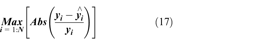
Maximum Relative Residual is the maximum distance out of all generated points from the calculated response surface to each generated point. The best value is 0%. In general, the closer the value is to 0%, the better quality of the response surface.

$$\underset{\mathit{i}=1:\mathit{N}}{\mathit{Max}}\left[\mathit{Abs}\left(\frac{{\mathit{y}}_{\mathit{i}}-\stackrel{\wedge }{{\mathit{y}}_{\mathit{i}}}}{{\mathit{y}}_{\mathit{i}}}\right)\right]$$

(17)

Root mean square error

For regression methods, the root mean square error is the square root of the average square of the residuals at the DOE points. The best value is 0. In general, the closer the value is to 0, the better quality of the response surface.

$$\sqrt{\frac{1}{\mathit{N}}\sum _{\mathit{i}=1}^N{\left(\frac{{\mathit{y}}_{\mathit{i}}-{\hat{\mathit{y}}}_{\mathit{i}}}{{\mathit{y}}_{\mathit{i}}}\right)}^2}$$

(18)

The error comparison of the three response surface models is shown in Table 7 and Figure 11. The total error of the Kriging method is the smallest, while that of the Sparse Grid method is larger. The amount of data to be calculated by the three methods is shown in Table 8. The Sparse Grid method needs to calculate the largest amount of data, and Kriging and Neural Network methods have the same amount of data. Considering the fitting precision and calculation efficiency, the Kriging method is more suitable for constructing the response surface model of pump performance simulation.

Table 7.

The error of three methods.

	Maximum relative residual (%)		Relative root mean square error (%)
	Pressure increment	Efficiency	Pressure increment	Efficiency
Sparse Grid	2.582	1.728	1.48	0.605
Kriging	1.4060	1.133	0.456	0.307
Neural Network	2.458	0.7	0.677742	0.292

Figure 11.

The error histogram.

Table 8.

Amount of data to be calculated by the three methods.

	Refinement points	Verification points	Total
Sparse Grid	96	30	126
Kriging	56	30	86
Neural Network	56	30	86

Optimization design

The optimal response surface model is optimized by using the multi-objective genetic algorithm MOGA. The initial sample number of the MOGA algorithm is 300, the sample number of each iteration is 100. The maximum allowable Pareto percentage is 80%, the convergence stability percentage is 2%, the maximum number of iteration steps is 20, the mutation probability is 0.01, and the crossover probability is 0.98. After 24 iterations, the Pareto front is obtained and shown in Figure 12. In the optimal design, the optimization objective is to maximize the pump efficiency and pressure increment at the same time, but the two optimization objectives are contradictory to some extent. We must make trade-offs and compromises between our objectives. Here we selected the result with high-pressure increment as the optimal solution on the premise of ensuring efficiency according to the engineering requirement.

Figure 12.

Pareto fronts of two objectives.

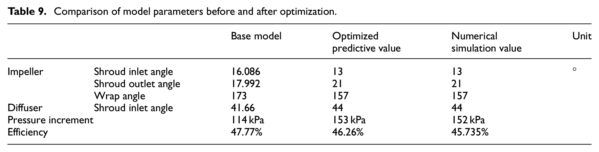
The optimal solution of the optimized design is numerically simulated. The final simulation results obtained are shown in Table 9. After optimization, the pressure increment is increased by 38 kPa, and the efficiency is reduced by 2.035%. The pressure increment is improved significantly, the efficiency is reduced less, the overall performance is greatly improved.

Table 9.

Comparison of model parameters before and after optimization.

		Base model	Optimized predictive value	Numerical simulation value	Unit
Impeller	Shroud inlet angle	16.086	13	13	°
	Shroud outlet angle	17.992	21	21
	Wrap angle	173	157	157
Diffuser	Shroud inlet angle	41.66	44	44
Pressure increment		114 kPa	153 kPa	152 kPa
Efficiency		47.77%	46.26%	45.735%

In this chapter, three different approximate models are constructed based on the experimental design points constructed by the sparse grid method, and the precision and computational efficiency of different approximate models are compared and analyzed. It is concluded that the Kriging model has high precision and less computation. The Kriging response surface model was optimized by the MOGA method, and the optimized results were verified by numerical simulation. The gas-liquid mixed transport performance has been improved.

Result and discussion

This chapter will compare and analyze the gas-liquid mixed transport performance of the multiphase pump before and after optimization, and analyze the reasons for the change of the performance.

Firstly, the optimized model was numerally simulated and the pump performance curve was obtained under the condition of GVF = 0.1–0.3, as shown in Figure 13(a). We can obtain from the figure that the pressure increment and efficiency gradually decrease with the increase of GVF. Figure 13(b) and (c) show the comparison diagram of pressure increment and efficiency before and after optimization under different GVF. It can be seen from Figure 13(b) that the pressure increment at the design point is greatly improved compared with the base model, and the optimized pump can achieve higher pressure increment in a wider flow range. We can obtain from Figure 13(c) that the optimized efficiency curve is slightly smaller at the design point than before. But in the large mass flow rate area, the efficiency is significantly improved, and the working efficiency range of the multiphase pump is broadened. It can be concluded from Figure 13(b) and (c) that when the flow rate is 1.3Q, the pressure increment and efficiency of the model pump are very low and can hardly work, while the optimized model can still work effectively. So we can conclude that the performance of the optimized multiphase pump has been significantly improved.

Figure 13.

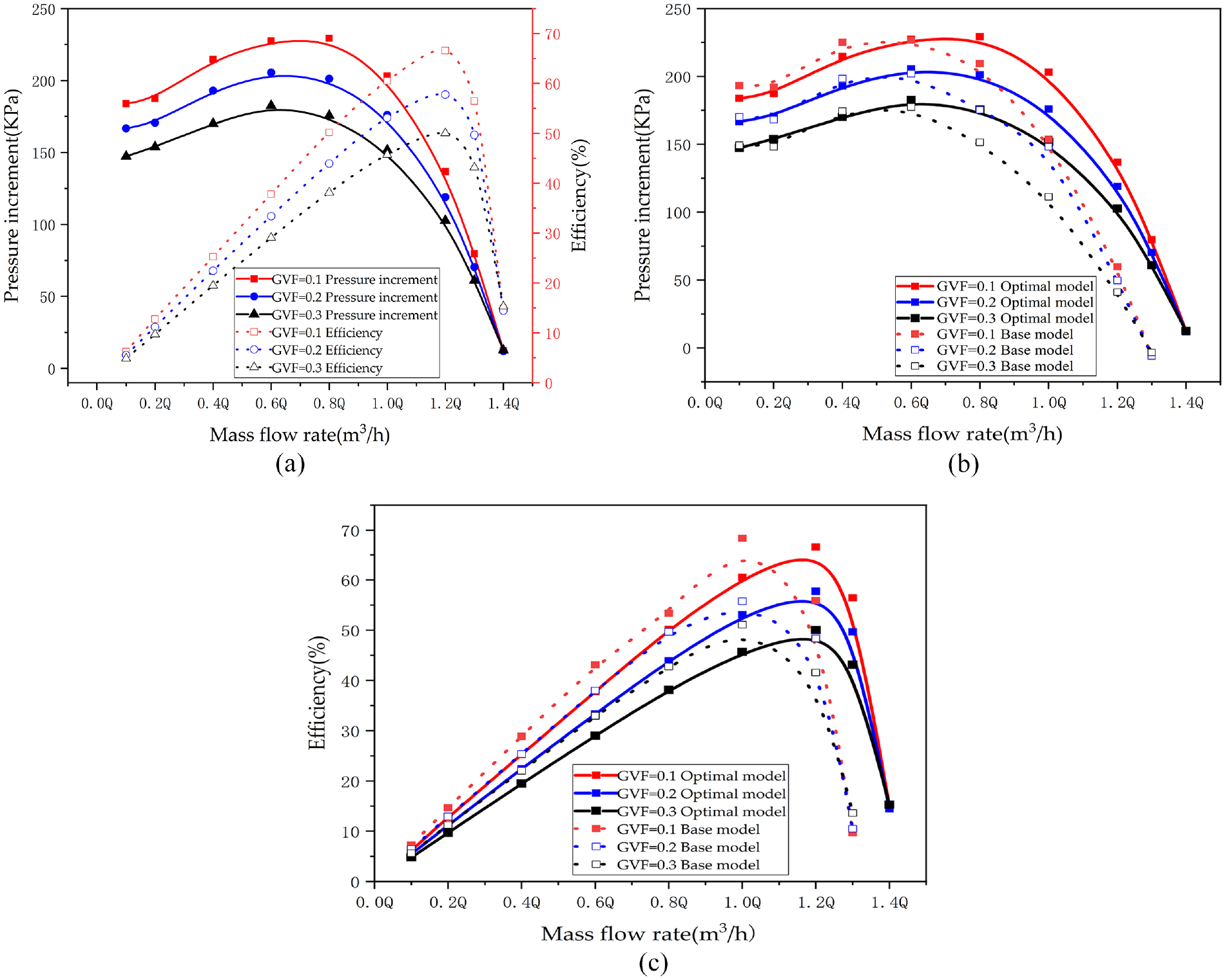
(a) The performance curve of the optimized pump with GVF from 0.1 to 0.3. (b) Pressure increment changes before and after optimization with GVF from 0.1 to 0.3. (c) Efficiency changes before and after optimization with GVF from 0.1 to 0.3.

Figure 14 shows the variation of impeller surface load before and after optimization. It can be concluded from the figure that the surface load on the inlet area of the impeller working face increases suddenly. Because when the fluid enters the inlet area of the impeller, it has a strong impact on the high-speed rotating impeller. The load on the pressure surface and suction surface in the impeller outlet area decreases slightly, which is mainly due to the vortex at the dynamic and static interface, resulting in energy loss. The load on the suction surface of the front half of the impeller is less than that on the pressure surface, while the load on the pressure surface of the rear half of the impeller is closer to that on the suction surface. It shows that the main part of the conversion of mechanical energy and pressure energy of a multiphase pump is the front half of the impeller. The optimized blade has higher static pressure, so the energy conversion characteristics are better. The load curve of the rear half of the impeller pressure surface is relatively flat, resulting in less flow loss, so the performance is better. It can be concluded from Figure 15 that the pressure increment of the impeller after optimization is significantly greater than that before.

Figure 14.

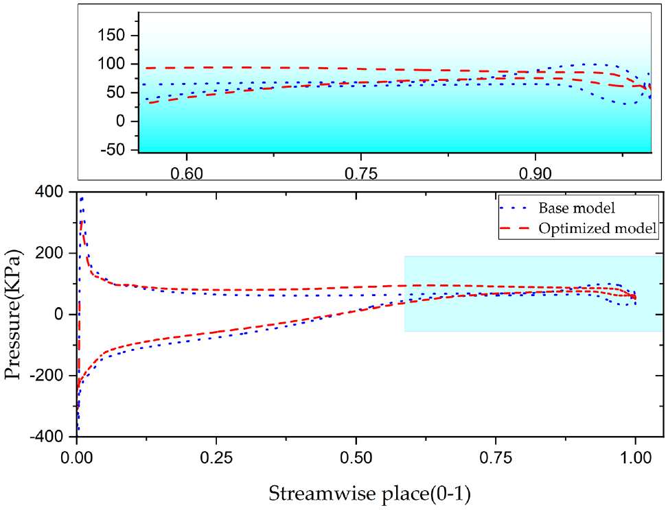
Blade load distribution with GVF = 0.3 on 50% span.

Figure 15.

Pressure increment of impeller before and after optimization.

Figure 16 shows that the high pressure area of the pressure surface of the optimized model increases, and the distribution from the inlet to the outlet of the impeller is more uniform. The results show that the optimized blade has better pressure increment performance. This is also consistent with the results in Figure 15.

Figure 16.

Surface pressure distribution of impeller pressure surface.

Figure 17 compares the streamline diagram of the multiphase pump at the design point from 10% span to 95% span before and after optimization. It can be seen that with the increase of blade height, the separated flow on the suction surface of the diffuser decreases gradually. The main reason is that due to the rotation of the impeller, a large number of high-density liquids are distributed in the parts with bigger blade span, and a large number of low-density gases are distributed in the parts with smaller blade span. The separation flow on the suction surface of the optimized diffuser is more serious than that before the optimization. After optimization, the pressure increment of the impeller area increases. The parameter change of the diffuser is not sufficient to deal with the sudden increase in pressure increment, so a pressure difference will be generated. Eventually led to the intensification of separation. This is also the main reason for the reduction of the efficiency of the multiphase pump at the design point after optimization.

Figure 17.

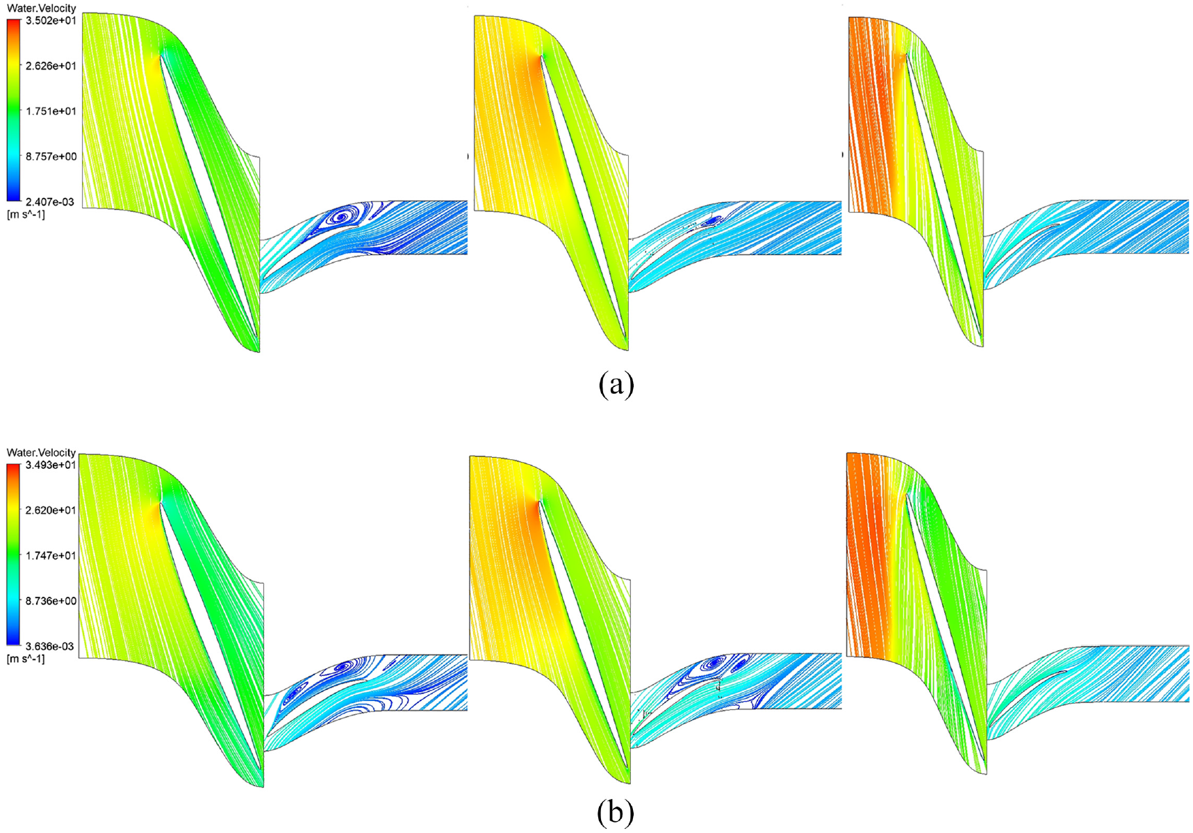
Streamline of blade height from 10% span to 95% span at Q. (a) 10% span, 50% span, and 95% span for model pump; (b) 10% span, 50% span, and 95% span for optimized pump.

Figure 18 shows the streamline distribution of the multiphase pump before and after optimization under the condition of 1.2Q. The results show that when the blade height is small (10%–50% span), the vortex formed by flow separation is effectively improved. It consumes less energy, so it is more efficient. This is also consistent with the curve in Figure 13(c).

Figure 18.

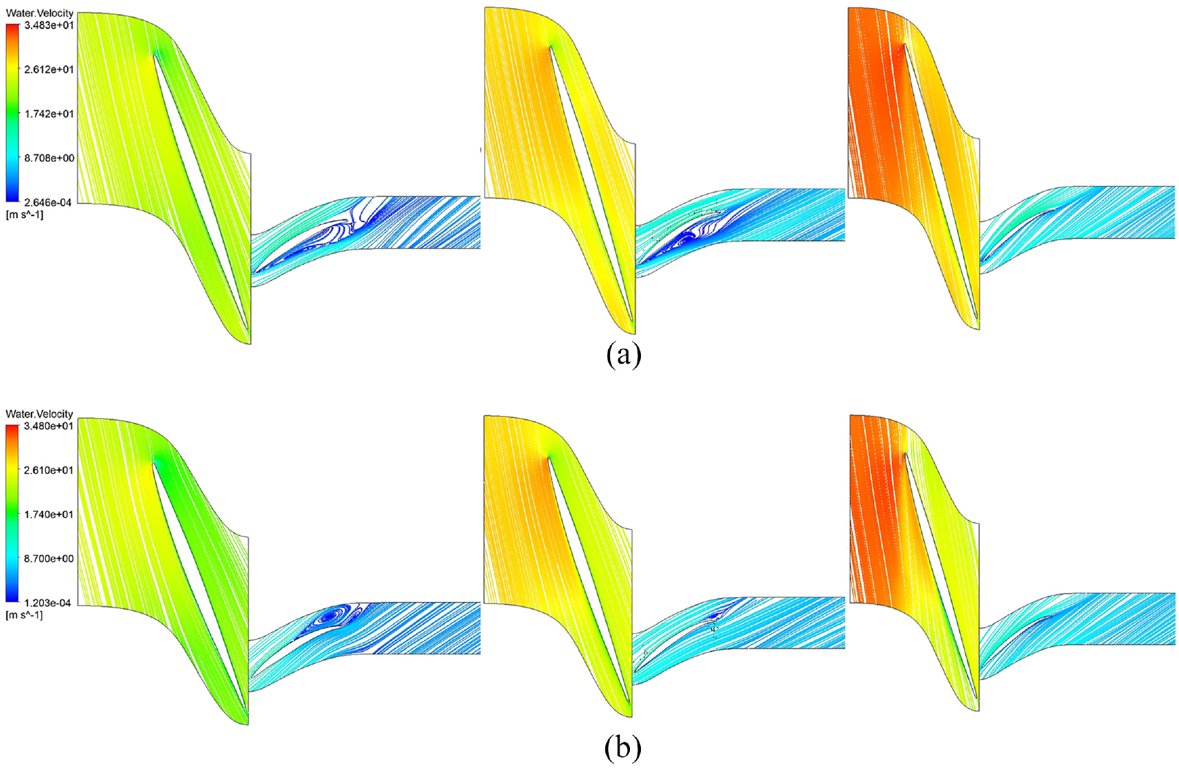
Streamline of blade height from 10% span to 95% span at 1.2Q. (a) 10% span, 50% span, and 95% span for model pump; (b) 10% span, 50% span, and 95% span for optimized pump.

Conclusions

Based on the design theory of axial flow pump and centrifugal pump inducer, a model pump was designed in this paper. Under the water condition and the condition of 10%–30% GVF, the numerical simulation of the model pump was carried out, and the characteristic curves of the model pump under various working conditions were obtained. The whole machine experiment is carried out to verify the hydraulic performance of the model pump.

The sparse grid method is introduced to construct a design of experiment for the structural parameters of the model pump. The approximate models are constructed by using the adaptive refined method of the Kriging, the Sparse Grid, and the Neural Work, respectively. The advantages and disadvantages of the three approximate models are compared and analyzed. The maximum correlation errors of the Kriging model in pressure increment and efficiency are 1.4060% and 1.133% respectively, and the root mean square errors are 0.456% and 0.307% respectively. Compared with the other two approximate models, it has fewer calculation data and high precision, so it is more suitable for building an approximate model for multiphase pump simulation.

The Kriging model is optimized under the working condition of 30% GVF by using the MOGA method. The pressure increment of the optimized model at the design point is 152 kPa, which is 38 kPa higher than the model pump. The efficiency is 45.735%, which is slightly lower than that before optimization. But the efficiency of the optimized model is significantly improved in large flow areas. When the mass flow rate is 1.2Q, the efficiency of the basic model is 38.61%, and the efficiency of the optimized model is 49.67%, and the efficiency is increased by 11.06%. When the flow is 1.3Q, the efficiency of the model pump is 12.71%, which can hardly work. While the optimized model efficiency is 43.06%, which can still work effectively. The internal flow field characteristics of the two models before and after optimization are compared and analyzed. After optimization, the surface load distribution of the impeller blade is more uniform, and the pressure increment of the impeller increases significantly. Under the condition of 1.2Q, the flow separation of the optimized model has been significantly improved, especially in the area where the blade height is small.

In this paper, the shape parameters of the impeller and diffuser of the multiphase pump are co-optimized by using an adaptive refined response surface method. At the design point, the pressure increment is significantly improved and the efficiency is slightly reduced. Under the condition of large mass flow, the efficiency is improved significantly, and the high-efficiency area of the multiphase pump is widened. Therefore, the optimization method in this paper is effective.