Flutter speed prediction by using deep learning

Abstract

Deep learning technology has been widely used in various field in recent years. This study intends to use deep learning algorithms to analyze the aeroelastic phenomenon and compare the differences between Deep Neural Network (DNN) and Long Short-term Memory (LSTM) applied on the flutter speed prediction. In this present work, DNN and LSTM are used to address complex aeroelastic systems by superimposing multi-layer Artificial Neural Network. Under such an architecture, the neurons in neural network can extract features from various flight data. Instead of time-consuming high-fidelity computational fluid dynamics (CFD) method, this study uses the K method to build the aeroelastic flutter speed big data for different flight conditions. The flutter speeds for various flight conditions are predicted by the deep learning methods and verified by the K method. The detailed physical meaning of aerodynamics and aeroelasticity of the prediction results are studied. The LSTM model has a cyclic architecture, which enables it to store information and update it with the latest information at the same time. Although the training of the model is more time-consuming than DNN, this method can increase the memory space. The results of this work show that the LSTM model established in this study can provide more accurate flutter speed prediction than the DNN algorithm.

Introduction

The aeroelastic flutter is a dynamic instability of a flight vehicle associated with the interaction of aerodynamic, elastic, and inertial forces. The flutter phenomenon is a self-excited destructive oscillatory instability. As the aerodynamic force exerted on the flexible body is coupled with its natural vibration mode, the vibration amplitude increases. Flutter speed is the critical speed when the flutter just occurs. Nearly 80% of aeroelastic flutter analysis in the industry is based on classical flutter analysis (CFA). ¹ The objective of the CFA is to determine the flight conditions that correspond to the flutter boundary. The flutter boundary corresponds to the conditions for which the aircraft is sustaining a simple harmonic motion. In the past decades, among many methods for analyzing flutter phenomena, P, K, and P-K methods are more practical and well known. ¹ Bisplinghoff et al. ² not only studied flutter phenomena and explained the physical meaning of flutter, but also made great contributions to flutter analysis, prediction of structural divergence and control of aeroelastic structures. Based on the complexity of aeroelastic coupling, Pitt and Haudrich ³ used the artificial neural network to analyze various flutter phenomena. Due to the difficulty in establishing computer instruction cycles and data at that time, the accuracy was not high, but it has inspired the follow-up research direction. In recent years, machine learning has developed vigorously. For example, Google recently defeated top Go players with AlphaGo ⁴ artificial intelligence Go software. Besides, deep learning methods are also widely used in image recognition, voice recognition, and data analysis and processing. In fact, the concept of “artificial intelligence” was put forward by American scholar John McCarthy in 1955. Around the 21st century, the development of artificial intelligence has undergone major changes. Hao ⁵ showed the design concept of artificial intelligence, which transits from establishing a large number of rules and system knowledge to machine learning. Machine learning is a branch of artificial intelligence. The concept of machine learning is to use different algorithms to establish a set of systems that can enable computers to learn automatically, and the cognitive model trained by this can predict and judge unknown data. Deep learning (DL) is a branch of machine learning, which was first proposed by Hinton et al. ⁶ in 2006. The concept of DL is to superimpose multiple hidden layers to simulate the neural network of the human brain for learning, but it also has the risk of over-fitting. Therefore, Hinton et al. also proposed the concept of dropout^7,8 to improve the phenomenon of over-fitting. The concept of dropout is to randomly discard some neurons during the training process of the neural network, thereby reducing the risk of over-fitting. Recently, both Li et al. ⁹ and Halder et al. ¹⁰ used the deep long short-term memory (LSTM) networks to analyze the aeroelastic effects on the bridge and airfoil, respectively. They both used the high-fidelity computational fluid dynamics (CFD) to establish their fluid-solid coupled models. CFD uses computers to perform the calculations required to simulate the free-stream flow of the fluid. Most of the computing time is used to calculate the interaction of the fluid with the solid surface defined by the boundary conditions. With high-speed supercomputers, better solutions can be achieved. It is commonly known that the CFD method is time consuming ¹¹ and is difficult to build the big data for machine learning. Ziaei et al. ¹¹ used the machine learning method to predict non-uniform steady turbulent flows in a 3D domain. Their proposed method provides an easy way for the designers and engineers to generate immense amounts of design alternatives without facing the time-consuming task of evaluation and selection.

In the development of modern deep neural networks (DNNs), feature learning and classification applications are even more outstanding. AlexNet ¹² won the ImageNet LSVRC title in 2012. GoogLeNet ¹³ won the championship in the ILSVRC competition in 2014. They achieved an error rate of only 6.67% using a 22-layer neural network architecture, which indirectly proves that increasing the number of layers of neural networks can describe complex models more accurately and bring better accuracy.

Hochreiter and Schmidhuber ¹⁴ improved the recurrent neural network (RNN) algorithm and proposed a long short term memory (LSTM) model. This model has a longer-term memory ability than the recurrent neural network. In recent years, Li et al. ⁹ and Halgan et al. ¹⁵ have used computational fluid dynamics (CFD) method to build long short term memory network models and analyze the aeroelastic phenomena of bridges and airfoils. In the framework of deep learning, long term short term memory models can process a large amount of data and learn more hidden information from non-linear systems. ¹⁶

In order to analyze flutter speeds under various flight conditions, this study adopted K method of flutter analysis method to analyze the occurrence of flutter speeds and build a large amount of data. The K method is a semi-analytical and numerical method. This method needs to establish the mathematical model and also needs computer coding to find flutter speeds. Most importantly, the flutter speed can only be predicted by K method case by case each time. Once the data bank was established, using the deep learning method can be efficiency and easier in predicting the results. The present study uses the DNN algorithm of machine learning to process complex aeroelastic model by superimposing a multi-layer neural network architecture. Referring to Hagan et al. ¹⁵ ’s research on neural network architecture, the present study designed a set of machine learning methods for computers to find rules from tens of thousands of flight data and obtain a set of classification methods. At the same time, this research also uses the LSTM algorithm to establish a deep learning model, and compares the advantages and disadvantages of DNN and LSTM. The supervised learning was used to guide the machine to recognize the learning target with Labels. Among many programming languages, Python has the highest support at present.^17,18 Python has a large number of third-party modules and a powerful standard library in order to use extended modules of other programming languages. This study used this tool as the basis. Under such analysis, the deep learning network can extract the features from various flight data, and find the flutter speed of the aircraft under different flight conditions. Finally, the theoretical predictions from the K method were applied to verify the learning status of deep learning and analyze the effectiveness of deep learning.

Introduction to the basic theory

Among many flutter analysis methods, P-K method is often used for analysis. Compared with P-K method, the K method occasionally misjudges the degree of freedom of structure flutter when analyzing aeroelastic problems.^1,19 However, this study only considered flutter speed, and did not focus on the flutter related to different degrees of freedom. Therefore, using K method will not affect the prediction of flutter speed, and can save much time when generating a large amount of flutter data.

Aeroelastic equations of motion for two-dimensional airfoils

Referring to the theory of flutter analysis proposed by Hodges and Pierce, ¹ we analyzed the flutter phenomenon of an airfoil, in which this model includes two degrees of freedom: plunge, and pitch. We assumed that these two degrees of freedom are subjected to springs K_h and $K_{\alpha }$ respectively, and this model is shown in Figure 1.

Figure 1.

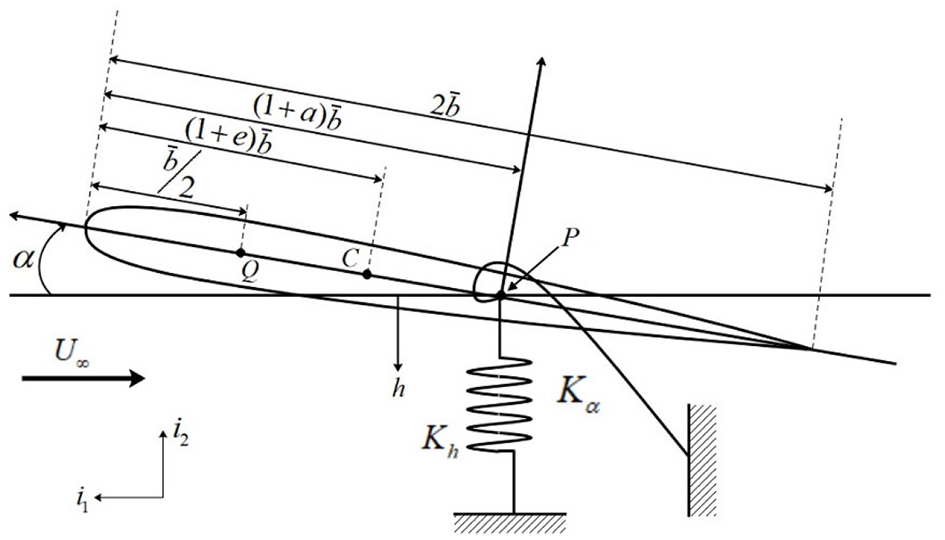
Schematics of the airfoil.

Here, Q in Figure 1 is the aerodynamic center. The aerodynamic center is the point that the pitching moment for the airfoil does not vary with lift, and usually defines as dC_m/dC_L=  0, where C_m is the pitching moment coefficient, C_L is the lift coefficient. C is the center of mass, and P is the elastic axis $\overline{b}$ is the half chord length of the airfoil, e is the location of elastic axis, a is the location of C.G., $\alpha$ is airfoil pitching motion. The dimensionless parameters e and a are between 1 and −1. If e is smaller than 0, it means that the centroid is located closer to the leading edge (LE). If e is larger than 0, it means that the center of mass is located closer to the trailing edge (TE). If e is 0, it means that the centroid position is at the position of half chord; if a is smaller than 0, it means that the elastic axis is located closer to LE. If a is larger than 0, it means that the elastic axis is located closer to TE. If a is 0, it means that the position of the elastic axis is on the half chord position.

Through Euler-Lagrange equation, we can get the basic Airfoil equation of motion as follows ¹ :

$$m(\stackrel{··}{h}+\overline{b}{x}_{\alpha }\stackrel{··}{\alpha })+K_{h}h=-L$$

(1)

$$I_p\stackrel{··}{\alpha }+m\overline{b}{x}_{\alpha }\stackrel{··}{h}+K_{\alpha }\alpha =M$$

(2)

where, m is the mass of airfoil, I_p is the moment of inertia of the airfoil, $x_{\alpha }=e-a$ is expressed as static unbalance parameter. If this parameter is positive, it means that the position of the elastic axis is forward from the position of the center of mass. The L and M are the lift and aerodynamic moment generated by the aerodynamic action of the airfoil. L and M can be expressed in the following form:

$$L=2\pi {\rho }_{\infty }b{U}^2\alpha$$

(3)

$$M=M_{\frac{1}{4}}+\overline{b}(\frac{1}{2}+a)L$$

(4)

$$M_{\frac{1}{4}}=0$$

(5)

Then ${\omega }_h=\sqrt{\frac{K_h}{m}}$ , ${\omega }_{\alpha }=\sqrt{\frac{K_{\alpha }}{I_p}}$ , after simplification, combining equations (1) and (2) with equations (3)–(5), the matrix form of the equation of motion of the airfoil can be obtained as follows:

$$\begin{array}{c}\left(\begin{array}{cc}m{\overline{b}}^2\hfill & m{\overline{b}}^2{x}_{\alpha }\hfill \\ \multicolumn{1}{c}{m{\overline{b}}^2{x}_{\alpha }}& I_p\hfill \end{array}\right)\left(\begin{array}{c}\frac{\stackrel{··}{h}}{\overline{b}}\hfill \\ \multicolumn{1}{c}{\stackrel{··}{\alpha }}\end{array}\right)\hfill \\ +\left(\begin{array}{cc}m{\overline{b}}^2{{\omega }_h}^2\hfill & 2\pi {\rho }_{\infty }{\overline{b}}^2{U}^2\hfill \\ \multicolumn{1}{c}{0}& \begin{array}{c}(-1-a)\pi {\rho }_{\infty }{\overline{b}}^2{U}^2\hfill \\ \multicolumn{1}{c}{+I_p{{\omega }_{\alpha }}^2}\end{array}\hfill \end{array}\right)\left(\begin{array}{c}\frac{h}{\overline{b}}\hfill \\ \multicolumn{1}{c}{\alpha }\end{array}\right)=\left(\begin{array}{c}0\hfill \\ \multicolumn{1}{c}{0}\end{array}\right)\hfill \end{array}$$

(6)

K method

K method is to add the artificial damping term to the right of the original aeroelastic equation of motion. By observing the variation of artificial damping, we can judge the divergence trend of the structure. Because K method is not like the general classical flutter analysis method, which needs a lot of iteration to calculate flutter speed, the K method is also the most efficient among many classical flutter analysis methods. Therefore, we chose K method to establish and verify the deep learning model in this study.

After adding artificial damping term ( $F_{D_h}$ and $F_{D_{\alpha }}$ ) to the right of equations (1) and (2), we can obtain the following equations:

$$m(\stackrel{··}{h}+\overline{b}{x}_{\alpha }\stackrel{··}{\alpha })+K_{h}h=-L+F_{D_h}$$

(7)

$$I_p\stackrel{··}{\alpha }+m\overline{b}{x}_{\alpha }\stackrel{··}{h}+K_{\alpha }\alpha =M+F_{D_{\alpha }}$$

(8)

We used simple harmonic motion to express the plunge motion (h) and pitch motion ( $\alpha$ ) of this model, and its lift (L) and aerodynamic moment (M). They are expressed as follows: $h(t)=\overline{h}{e}^{i\omega t}$ , $\alpha (t)=\overline{\alpha }{e}^{i\omega t}$ , $L(t)=\overline{L}{e}^{i\omega t}$ , $M(t)=\overline{M}{e}^{i\omega t}$ . $F_{D_h}$ and $F_{D_{\alpha }}$ can be expressed in the following forms:

$$F_{D_h}=-i{\overline{g}}_h\overline{h}{e}^{i\omega t}$$

(9)

$$F_{D_{\alpha }}=-i{\overline{g}}_{\alpha }\overline{\alpha }{e}^{i\omega t}$$

(10)

After substituting $\mu =\frac{m}{\pi {\rho }_{\infty }{\overline{b}}^2}$ , $r=\sqrt{\frac{I_p}{m{\overline{b}}^2}}$ , $\hat{\sigma }=\frac{{\omega }_h}{{\omega }_{\alpha }}$ into equations (7) and (8), we can obtain the following equation:

$$\begin{array}{c}\left(\begin{array}{cc}\begin{array}{c}\mu [1-{\hat{\sigma }}^2{\left(\frac{{\omega }_{\alpha }}{\omega }\right)}^2(1+i{g}_h)]\hfill \\ \multicolumn{1}{c}{+l_h(k,M_{\infty })}\end{array}\hfill & \mu x_{\alpha }+l_{\alpha }(k,M_{\infty })\hfill \\ \multicolumn{1}{c}{\mu x_{\alpha }+m_h(k,M_{\infty })}& \begin{array}{c}\mu r^2[1-{\left(\frac{{\omega }_{\alpha }}{\omega }\right)}^2(1+i{g}_{\alpha })]\hfill \\ \multicolumn{1}{c}{+m_{\alpha }(k,M_{\infty })}\end{array}\hfill \end{array}\right)\hfill \\ \left(\begin{array}{c}\frac{\overline{h}}{\overline{b}}\hfill \\ \multicolumn{1}{c}{\overline{\alpha }}\end{array}\right)=\left(\begin{array}{c}0\hfill \\ \multicolumn{1}{c}{0}\end{array}\right)\hfill \end{array}$$

(11)

where, $k=\frac{\overline{b}\omega }{U}$ is the reduced frequency, $M_{\infty }=\frac{U}{C_{\infty }}$ is the Mach number.

After solving the determinant of equation (11), the flutter speed can be obtained. Figures 2 and 3 are the results of using K method to obtain flutter speed. From the change of artificial damping in Figure 2, it can be seen that artificial damping will change from negative value to positive value at the position of 4.6, which means that flutter will occur at the position of dimensionless flutter speed (1/k) = 4.6. Meanwhile, comparing with Figure 3, we can see the change trend of system frequency before and after flutter generation.

Figure 2.

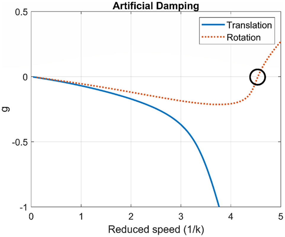
Artificial damping of K method prediction.

Figure 3.

Frequency of K method prediction.

Deep learning

This study used the deep learning algorithm to perform flutter speed analysis. The DNN architecture adopted herein is based on supervised learning, and a set of neural networks was designed to predict the results after repeated operations by a large number of artificial neurons. In this study, supervised learning in machine learning was adopted, so in building a learning model, besides the features of data, data labels should also be the input. Therefore, we needed to mark huge data, and the data marking in this study was based on K method of flutter analysis. We set the parameters used in the airfoil equation of motion in Section II as data features, and the flutter speed obtained by using K method was the data label. We used computer processing to carry out a large number of labels to avoid spending too much time on data collection. The parameters used in the learning model are the location of center of mass, the location of elastic axis, mass ratio, radius of gyration, frequency ratio, and static unbalance parameter. Table 1 is the parameter data used by the dataset. Finally, there are 350,892 data sets established in this study.

Table 1.

Parameters used by the dataset.

Variables in the flutter speed dataset
	Features						Label
	Location of c.g.	Location of elastic axis	Mass ratio	Radius of gyration	Frequency ratio	Static unbalance
	$a$	$e$	$\mu$	$r$	$\hat{\sigma }$	$x_{\alpha }$
Range	[−0.9, 0.9]	[−0.9, 0.9]	[5, 60]	[0.1, 0.9]	[0.1, 0.9]	[−1.8, 1.8]	[0, 100]

In the feature scaling of data, the data normalization method we used is Min-Max normalization, which scales the data to the [0, 1] interval in equal proportion to avoid the excessive contribution of a certain parameter, which affects the convergence speed of model building and further reduces the training efficiency. The expression of Min-Max normalization is as follows:

$$x\prime =\frac{x-x_{min}}{x_{max}-x_{min}}$$

(12)

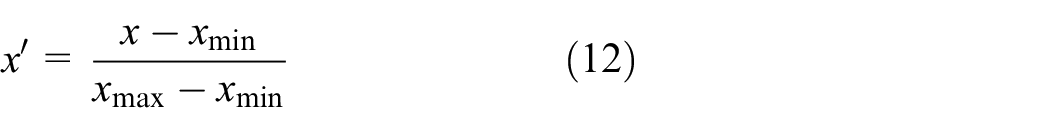
where, x′ denotes normalized data, x is raw data, x_min is the smallest data value in the raw data set, and x_max is the largest data value in the original data set.

Deep neural network (DNN)

DNN is a kind of Artificial Neural Network (ANN), also known as the Neural network. The concept of deep neural network is a neural network formed by a combination of a large number of neurons, which simulates the behavior of the human brain to transmit and process information through neuronal connections to respond or solve problems. In the basic architecture of a deep neural network, there are multiple hidden layers between the input layer and the output layer, and each layer is composed of a large number of neurons, and all the neurons in the input layer are individually connected to the neurons in the hidden layer, and the neurons in the hidden layer are also individually connected to the output layer. The schematic diagram of the neural network-like structure is shown in Figure 4.

Figure 4.

The schematic diagram of the neural network-like structure.

Neural network is composed of many artificial neurons, in which each artificial neuron is connected with a weight value, and each artificial neuron has a deviation value. The relationship between the input value and the output value is generally expressed by the following form,

$$y=\sigma (\sum _{i=1}^n{w}_i{x}_i+b)$$

(13)

where x is the input value of the artificial neuron, w is the weight, b is the deviation value, y is a value obtained by multiplying each input value and weight value and summing it up with a given deviation value, $\sigma$ is the activation function (AF). After obtaining the summation of weighted inputs and deviation value, it needs to be converted by an activation function. The AFs used in this paper are Sigmoid function, Rectified Linear Unit (ReLU) function, and Softmax function, where the above AFs are respectively represented as follows, $\sigma (\mathrm{z})=\frac{1}{1+e^{-z}}$ , $\sigma (\mathrm{z})=max(0,z)$ , $\sigma {(\mathrm{z})}_i=\frac{e^{z_i}}{\sum _{j=1}^n{e}^{z_j}}$ .

Long short term memory (LSTM)

LSTM uses three control gates to learn and achieve the effect of long-term memory, and these three control gates will determine the storage and use of memory, which are Input gate, Forget gate, and Output gate. Figure 5 is a schematic diagram of the LSTM model. When a long-term and short-term memory model is operating, the hidden state at the previous time state and the current input value will be entered into the long-term and short-term memory for calculation at the same time, which will be multiplied by a weighting value and added to a deviation value. Then, the conversion is performed through the activation functions of the input gate, the forget gate, and the output gate. The activation functions are all sigmoid functions, and the updated cell state uses the hyperbolic tangent function as the activation function. The calculations are shown as follows:.

$$I_t=\sigma (w_{\mathrm{IX}}\left[X_t\right]+b_I+w_{\mathrm{Ih}}\left[h_{t-1}\right]+b_I)$$

(14)

$$F_t=\sigma (w_{\mathrm{FX}}\left[X_t\right]+b_F+w_{\mathrm{Fh}}\left[h_{t-1}\right]+b_F)$$

(15)

$$O_t=\sigma (w_{\mathrm{OX}}\left[X_t\right]+b_O+w_{\mathrm{Oh}}\left[h_{t-1}\right]+b_O)$$

(16)

$${\overline{C}}_t=\tanh (w_{\mathrm{CX}}\left[X_t\right]+b_C+w_{\mathrm{Ch}}\left[h_{t-1}\right]+b_C)$$

(17)

Figure 5.

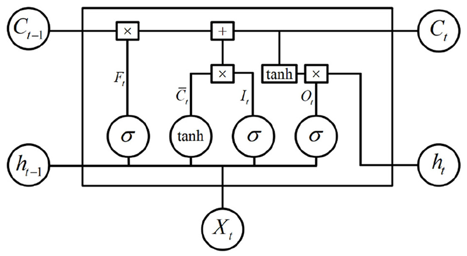
LSTM model.

where I_t is the information passing through the input gate, F_t denotes the information passing through the forgotten gate, O_t represents the information passing through the output gate, ${\overline{C}}_t$ is the updated unit state, X_t represents the current input value, and h_t-1 denotes the previous hidden state. Then the result of the input gate and the forgetting gate will determine how to update the cell state transferred to the next long and short-term memory. If the value converted by the activation function of the forgotten gate is 0, it means that the unit state at the last time point is cleared. If the value converted by the activation function of the input gate is 0, it means that the current information has not passed the input gate. Therefore, the cell state calculated from the hidden state at the last time point and the current input value will not be used, and the updated cell state calculation is shown in equation (18).

$$C_t=F_t\odot C_{t-1}+I_t\odot {\overline{C}}_t$$

(18)

C_t is not only the updated cell state, but also the cell state transferred to the next long and short-term memory. Finally, the result of the output gate calculation will determine how to update the hidden state. If the value of the activation function converted by the output gate is 0, it means that the current unit state cannot pass the output gate, so the hidden state will not be recorded. The updated hidden state expression is shown in equation (19).

$$h_t=O_t\odot \tanh \left(C_t\right)$$

(19)

At this point, the long and short-term memory unit has been completely trained. The LSTM method uses memory units and hidden states to increase the dependence of data training. Therefore, we use the LSTM method to establish the deep learning model to predict the flutter speed.

Loss function

The loss function we used in deep neural networks is categorical cross-entropy. It is applicable to a variety of classification problems. We also use Softmax function as the activation function of the output layer. The calculation of categorical cross entropy is shown in equation (20).

$$E_D=-\sum _i^n{y}_i\log (p_i)$$

(20)

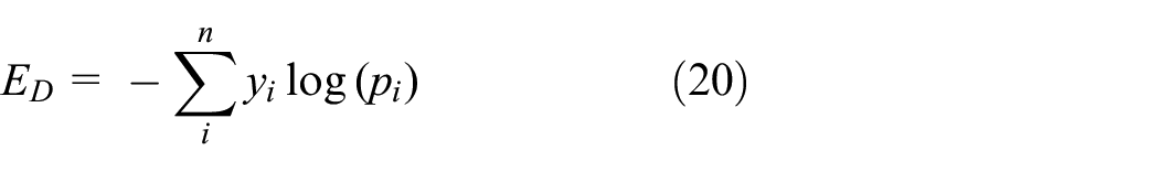
where n is the number of classification categories, y_i is the label of the data, and p_i is the accuracy of the classifier in predicting the occurrence of flutter speed. In LSTM method, we used the mean square error (MSE) to evaluate the error of the training model. This method is a commonly used regression loss function. This is a commonly used regression loss function. The calculation of the mean square error is shown in equation (21).

$$E_L=\frac{1}{q}{\sum }_{i=1}^q{(y_i-{\hat{y}}_i)}^2$$

(21)

where q is the total number of data, y_i is the label of the data, and ${\hat{y}}_i$ is the predicted value.

Back propagation

Back propagation is a sequential transmission from the output layer to the input layer, and the difference between the training data converted by the activation function and the corresponding input target value is obtained, thus obtaining the loss function gradient related to each weight parameter. Here, input training data is converted through AF and we can obtain $y=\sigma (z)$ . The back propagation calculates and stores the loss function gradient in each neural network layer through the chain rule in calculus and the difference between the output value trained by the neural network and the exact output value, and repeatedly trains and adjusts until the relevant weight value tends to be stable. The gradient of the loss function in each neural network layer is as follows,

$$\frac{\partial S_L}{\partial w}=\frac{\partial z}{\partial w}\frac{\partial y}{\partial z}\frac{\partial S_L}{\partial y}$$

(22)

After obtaining the gradient of the loss function in each hidden layer, the weight can be updated by using the gradient of the loss function to obtain the best weight value. The loss function used by us in the DNN was categorical cross-entropy. Finally, the Softmax function was adopted as the AF of the output layer. The loss function of classification cross entropy is as follows.

$$S_L=-\sum _i^n{y}_i\log ({\hat{y}}_i)$$

(23)

where, n is the number of classification categories, y_i is the volume label of the data, ${\hat{y}}_i$  is the accuracy of flutter generation predicted by the classifier.

Other parameter setting

In the weight update of the DNN, we choose Adam method ²⁰ to calculate and adjust the weight value of the updated model. We chose Adam method for weight update because compared with other weight update methods, this method is easier to execute, has relatively high calculation efficiency, requires less memory, and is suitable for problems with a large amount of data and parameters. Adam related expressions are as follows.

$$m_t={\beta }_1{m}_{t-1}+(1-{\beta }_1)g_t$$

(24)

$$v_t={\beta }_2{v}_{t-1}+(1-{\beta }_2){g_t}^2$$

(25)

where, new representations ${\hat{m}}_t$ and ${\hat{v}}_t$ can be obtained by performing deviation correction on equations (24) and (25). The representations are as follows,

$${\hat{m}}_t=\frac{m_t}{1-{{\beta }_1}^t}$$

(26)

$${\hat{v}}_t=\frac{v_t}{1-{{\beta }_2}^t}$$

(27)

In equations (24) and (25), g_t is expressed as loss function gradient, $g_t=\frac{\partial S_{L_t}}{\partial w_t}$ . Then, new weights can be calculated by using equations (26) and (27), and the operation mode is as follows.

$$w_{t+1}=w_t-\frac{\eta {\hat{m}}_t}{\sqrt{{\hat{v}}_t+\epsilon }}$$

(28)

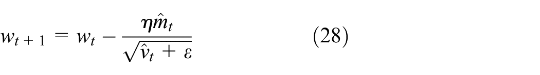
where m and v are parameters used to adjust the weight values of neural networks. Among them, the default value of ${\beta }_1$ is 0.9, and that of ${\beta }_2$ is 0.999, and $\epsilon$ is 1e−08. The learning rate in this study $\eta$ is set as 0.003.

Modeling and Analysis

DNN model

Based on the deep learning theory proposed in last Section and referring to Hagan and Schmidhuber’s ¹⁴ research on neural network architecture, this Section constructed a set of deep learning architecture that can predict flutter speed, and carried out deep learning on 350,892 flight data. Among them, 70% of the flight data are regarded as training set, 20% as validation set, and the remaining 10% as prediction data. In the design of architecture, we first established the most basic three-layer deep learning framework for test training. Among them, the starting function in the deep learning architecture uses ReLU function for training except for Softmax function in the output layer. After 10,000 Epoch training, the results obtained are not satisfied. The training accuracy and testing accuracy are stuck at 82%. The training results are shown in Figures 6 and 7.

Figure 6.

Accuracy of 1-layer deep learning architecture training.

Figure 7.

Loss of 1-layer deep learning architecture training.

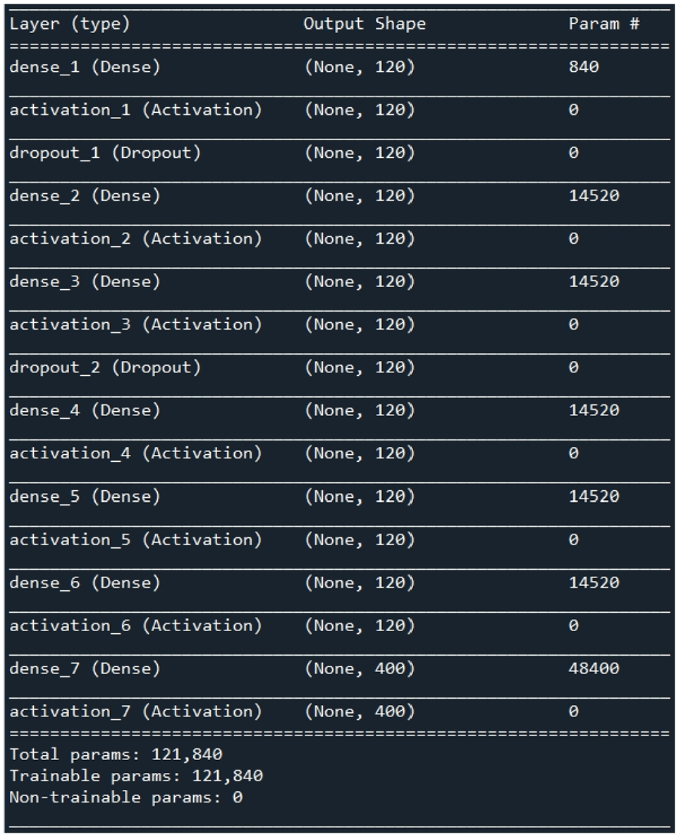
After the first test, we decided to increase the number of artificial neurons and the number of layers of deep learning architecture to achieve better accuracy. When a 7-layer deep learning architecture was used, after 10,000 Epoch training, the training accuracy has reached 97%, and the accuracy of verification reaches 94%. However, in the loss results, there is an increasing trend with the increase of Epoch. The reason is that the over-fitting phenomenon is due to the deep learning architecture stacking too many layers or using too many artificial neurons, which causes the noise in each data to be amplified when verifying the results, resulting in an increasing trend of loss. The training results are shown in Figures 8 and 9.

Figure 8.

Accuracy of 7-layer deep learning architecture training.

Figure 9.

Loss of 7-layer deep learning architecture training.

Figure 10 shows the training loss and testing loss results of different layers of neural network architecture. After many attempts (see Figure 10), we chose a 6-layer deep learning architecture and used Dropout ⁷ to improve the over-fitting phenomenon. Although its accuracy is not as high as that of the 7-layer deep learning architecture, it avoids the phenomenon of over-fitting. We adopted Sigmoid function, ReLU function, and Softmax function as the activation function of the model in this study. The Categorical cross-entropy was selected as the loss function of this model, and Softmax function as the starting function of the output layer. The activation function of each other layer uses Sigmoid function and ReLU function. Table 2 shows the results of model training loss under different combinations of Sigmoid and ReLU activation functions.

Figure 10.

Training loss and testing loss of different layers of neural network architecture.

Table 2.

Training loss results with different activation function combinations.

DNN training and testing loss with different activation function arrangement
Activation function	Layer 1–5: sigmoid	Layer 1: ReLU, layer 2–5: sigmoid	Layer 1–2: ReLU, layer 3–5: sigmoid	Layer 1–3: ReLU, layer 4–5: sigmoid	Layer 1–4: ReLU, layer 5: sigmoid
Training loss	0.2261	1.6089	1.6181	1.6229	0.1363
Testing loss	0.2508	1.6091	1.6257	1.6231	0.1803
	Layer 1–5: ReLU	Layer 1: sigmoid, layer 2–5: ReLU	Layer 1–2: sigmoid, layer 3–5: ReLU	Layer 1–3: sigmoid, layer 4–5: ReLU	Layer 1–4: sigmoid, layer 5: ReLU
Training loss	0.1636	0.1475	0.1508	0.2814	0.2921
Testing loss	0.2234	0.2041	0.2712	0.3474	0.3444

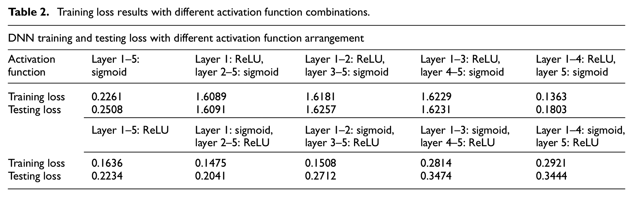
As shown in Table 2, when the ReLU function is used as the activation function in Layer 1 to Layer 4, and the Sigmoid function is used as the activation function in Layer 5, the loss of training results is the relatively lowest compared with other combinations, and its training loss is 0.1363, and the loss during verification is 0.1803. Therefore, this group of combination was chosen as the basis for establishing the deep learning model activation function of this study. After determining the activation function of the model in this study, we decided to train the model with different number of neurons and find out the number of neurons suitable for this model. Figure 11 is the result of training losses using different number of neurons. From the training loss results of different number of neurons, it can be seen that when the number of neurons increases, the training loss tends to decrease with the increase of the number of neurons. However, the loss of test tends to increase after 120 neurons, we then use 120 neurons to establish the deep learning model of this study. Based on the above results, we have established a 6-layer deep learning architecture, in which layers 1–5 use ReLU function as activation function, layer 6 uses Sigmoid function as activation function, the output layer uses Softmax function as activation function, the loss function uses Categorical cross-entropy method, and each layer is established with 120 neurons. Figure 12 is the framework of the deep learning model in this study, and the training results are shown in Figures 13 and 14, and the accuracy of the trained model is 95.6%. Although it is 1.4% lower than the previously established 7-layer deep learning architecture (97%), this model has higher robustness.

Figure 11.

Training loss results of different number of neurons.

Figure 12.

Deep learning model.

Figure 13.

Precision of deep learning architecture.

Figure 14.

Loss of deep learning architecture.

LSTM model

We regard 70% of the 350,892 flight data as the training set, 20% of the data as the validation set, and the remaining 10% as the predicted data and import them into the LSTM model for training. The input parameters of the LSTM model in this study are consistent with the DNN model. In the design of the LSTM architecture, we first established a basic single-layer deep learning architecture for testing and training, and then increased the number of layers of long-term and short-term memory. Finally, we chose to use five layers of long- and short-term memory as the LSTM model. The LSTM architecture test training results of different layers are shown in Figure 15.

Figure 15.

LSTM testing and training results of different layers.

Since the Sigmoid function and the hyperbolic tangent function have been used as the activation function in the LSTM model, we no longer use the activation function between the hidden layers to avoid excessive non-linear conversion between the hidden layers causing the output value to be distorted. In the training process, we also added a dropout layer between the hidden layers to prevent over-fitting. This study uses a 5-layer LSTM layer. Since the previous training has used a fixed number of LSTM cells, we will tune the number of LSTM cells to obtain the best number of long and short-term memory cells. Figure 16 shows the training loss results using different numbers of LSTM cells. From the training loss results of different numbers of long and short-term memory cells, it can be seen that when the number of cell is 80, the training loss and test loss are small, so we chose to use 80 cells to establish this deep learning model. Next step is to choose an appropriate number of epochs to train the LSTM model in this study. Figure 17 shows the loss and accuracy results of different epoch training. It can be seen from Figure 18 that the loss result after 3000 epochs training is low; however, when it is increased to 4000 epochs, the accuracy does not increase significantly. Therefore, we choose to use 3000 epochs to build the deep learning model of this research.

Figure 16.

LSTM training loss using different numbers of cells.

Figure 17.

Loss and accuracy of different epoch training.

Figure 18.

Architecture of the LSTM model.

Based on the above results, we have established a 5-layer LSTM architecture, in which the loss function uses the mean square error method, and each layer is built using 80 LSTM cells, and the number of training is 3000 epochs. Figure 17 is the architecture of the LSTM model of the present study. The average accuracy of the trained model is 96.8%. The accuracy and loss results of the training are shown in Figures 19 and 20.

Figure 19.

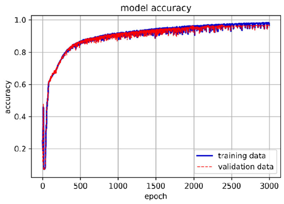
Accuracy of the LSTM training model.

Figure 20.

Loss of the LSTM training model.

Model prediction and result discussion

In this Section, the deep learning model obtained from last Section was used to predict flutter speed of various flight parameters. The verification results by DNN model are shown in Figure 21. Table 3 is the relevant data of this DNN model. In the verification result, an accuracy of 95.6% is achieved. It is noted that the red dots in Figures 21 and 22 indicate the results of the true flutter speed versus the predicted flutter speed, while the dashed line represents the ideal case of DNN (Figure 21) or LSTM (Figure 22) model prediction result. The verification results by LSTM model are shown in Figure 22. In the verification result, an accuracy of 96.8% is achieved. Again, the red dots in Figure 22 indicate the results of the true flutter speed versus the predicted flutter speed, while the dashed line represents the ideal case of LSTM model prediction result. The results show that the LSTM model has better accuracy than the DNN model.

Figure 21.

DNN prediction results.

Table 3.

DNN model data.

Variables information	Setting point
Algorithm	DNN
Number of samples	350,892
Classification	1–400
Average accuracy	95.6%

Figure 22.

LSTM prediction results.

Figures 23 to 27 are the prediction results of flutter speed after input and training of various parameters. Vertical axis is flutter speed. The higher the value is, the higher the flutter speed is. A higher flutter speed means that it is less likely to cause structure divergence. For each figure, (a) is the predicted results by DNN, and (b) is the predicted results by LSTM model. Figure 23 shows that this model has high stability if the center of mass locates from quarter chord to half chord, the estimated value is consistent with aeroelastic point of view. That is, when the center of mass is located in the front half of airfoil (quarter chord), the model has higher stability than the rear half. Figure 24 shows that the aeroelastic model is more stable when the position of elastic axis is placed near the quarter chord. It is true that from aerodynamic point of view, when the position of elastic axis is placed near the quarter chord, the system will have higher stability. Figure 25 is the relationship between mass ratio and flutter speed, where the mass ratio is expressed as $\mu =m/\pi {\rho }_{\infty }{b}^2$ . The mass ratio is a dimensionless parameter of air density. When the mass ratio is larger, it means that the air density is lower, and the energy obtained by the elastic structure from the air is greatly reduced, so the possibility of the occurrence of flutter decreases and the stability is higher. Figure 26 is the relationship between the radius of gyration and flutter speed, and the increase of rotation radius has a relatively stable trend, where the radius of gyration is expressed as $r=\sqrt{I_p/m{b}^2}$ . Thus, the radius of gyration is related to the moment of inertia. The larger the radius of gyration, the larger the moment of inertia, and the more stable the pitching motion is. Figure 27 is the relationship between static unbalance parameter and flutter speed. This value represents the distance between the center of mass position and the elastic axis position, and it is relatively stable when it is 0 to −1, which means that the elastic axis has relatively high stability when it is placed in front of the center of mass. This is also consistent with aeroelastic point of view, that is, the position of the elastic axis is placed in front of the center of mass, which has higher stability than when it is placed behind the center of mass. So far, the 6-layer DNN and LSTM methods we have established can provide accurate prediction of flutter speed.

Figure 23.

Relationship between location of center of mass and flutter speed, predicted by (a) DNN model and (b) LSTM model.

Figure 24.

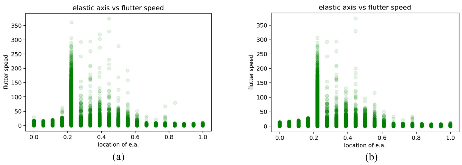
Relationship between location of elastic axis and flutter speed, predicted by (a) DNN model and (b) LSTM model.

Figure 25.

Relationship between mass ratio and flutter speed, predicted by (a) DNN model and (b) LSTM model.

Figure 26.

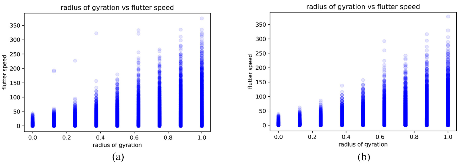
Radius of gyration and flutter speed, predicted by (a) DNN model and (b) LSTM model.

Figure 27.

Relationship between static unbalance and flutter speed, predicted by (a) DNN model and (b) LSTM model.

From Figures 23 to 27, we can see the trend of the flutter speed predicted by LSTM is consistent with the trend of the prediction result of the DNN model, and the prediction conditions of both can be explained by the physical meaning of aerodynamics and aeroelasticity. As far as the results of the current stage of this research are concerned, the prediction of flutter speed has reached a good level, among which the average prediction accuracy of the DNN model and the LSTM model have reached more than 95%. Figures 21 and 22 are the predictions by importing the same data set. From the two figures, it can be clearly judged that the deep learning model established by using the LSTM method is better than the deep learning model established by the DNN method. Moreover, most of the predictions of the LSTM model are closer to the theoretical flutter speeds than the DNN model. From Figures 23 to 27, the fluctuations of the flutter speeds predicted by the DNN model are larger than that of the LSTM model, and the robustness is also lower than that of the LSTM model. We believe that the reason for this result is that the LSTM model has a cyclic architecture, which enables it to store information and update it with the latest information at the same time. It also uses three control gates to adjust and select memory storage and access. Although the training of the model is more time-consuming than DNN, this method can increase the memory space. The DNN model is a feed-forward neural network. The data sets imported into this model are not well related. Although the accuracy of the DNN model has reached 95.6%, the prediction robustness of the DNN model is relatively low.

Conclusions

This study uses deep learning algorithms to analyze the aeroelastic phenomenon and compare the differences between Deep Neural Network (DNN) and Long Short-term Memory (LSTM) applied on the flutter speed prediction. Instead of time-consuming high-fidelity computational fluid dynamics (CFD) method, this study uses the K method to build the aeroelastic flutter speed big data for different flight conditions. The flutter speeds for various flight conditions are predicted by the deep learning methods and verified by the K method. The detailed physical meaning of aerodynamics and aeroelasticity of the prediction results are studied. The conclusions are listed below:

1. The number of layers and the number of neurons for the DNN and the LSTM will affect the accuracy of the model. Not that the more layers the better the effect. The number of neurons is not the more the better the effect. Too many layers or too many neurons will cause the model to produce over-fitting phenomenon, resulting in a decrease in the accuracy of the prediction results. A case analysis based on this research is necessary.

2. The number of epochs of the deep learning model in this study determines whether the model is fully trained, but if the epoch is set too large, it may cause the model to be over-fitted during the training process, which will affect the accuracy. At the same time, too many number of epochs will increase the calculation time and reduce the efficiency of training. Choosing the appropriate number of epochs will improve the efficiency of training.

3. The prediction results of the DNN and the LSTM deep learning models conform to the theoretical explanation of aeroelasticity and aerodynamics.

4. This study uses DNN and LSTM methods to build deep learning models, with an average accuracy of more than 95%. The LSTM model performs better than the model established by the DNN method, and its robustness is also higher.

In this study, DNN and LSTM are employed to predict the occurrence of flutter speed, both of the deep learning methods are used to learn the relation between each flight data and its associated flutter speed by considering this problem as a multi-class classification, so as to achieve the goal of this study. The results show that the LSTM architecture can effectively predict the flutter speed, and it is a potential model in the application of aerospace field.