Sage Journals: Discover world-class research

Abstract

Cognitive radio is a paradigm that proposes managing the radio electric spectrum dynamically by integrating the spectrum sensing, decision-making, sharing, and mobility stages. In the decision-making stage, the best available channel is selected for transmitting secondary user data in an opportunistic fashion, and the success of that stage depends on the efficiency of the primary user characterization model. Use of the long short-term memory technique based on the deep learning concept is proposed in order to reduce the forecasting error present in the future estimation of primary users in the GSM and WiFi frequency bands. The results show that long short-term memory has the capacity needed to improve channel use forecasting significantly more than other methods such as multilayer perceptron neural networks, Bayesian networks, and adaptive neuro-fuzzy inference systems (ANFIS-Grid). It is concluded that although long short-term memory exhibits better performance generating forecasts for time series, computing complexity is higher due to the existence of input, forget, and output gates within the neural structure; therefore, implementation is feasible in cognitive radio networks based on centralized network topologies.

Keywords

Cognitive radio neural network deep learning GSM long short-term memory

Introduction

In the same manner as land is more costly and scarce in urban areas due to the fact that they are densely populated (because of the quality of life they offer), the operating range of the radio electric spectrum is more useful in certain frequency bands than others because they facilitate the interconnection of devices and reduce the probability of errors. Wireless systems are currently characterized by a spectrum allocation policy that is established and regulated by the government of each country. This presents spectrum distribution issues (Figure 1)¹ because spectrum use is deficient due to large spatial and temporal variations in spectrum occupation.^2–4 A consequence of underutilization is a current spectrum shortage, which causes a significant degradation in the quality of service (QoS) offered by telecommunications companies (e.g. wireless band), an aspect that has motivated researchers from different fields to formulate possible solutions for optimizing spectrum use. Dynamic spectrum access is a solution, along with the cognitive radio (CR) concept, the main purpose of which is to identify spectrum holes not used by primary users (PUs) so that they can be used opportunistically by secondary users (SUs).

Figure 1.

Spectrum occupation in the 30 MHz to 3 GHz range.¹

CR can be defined as a system that is controlled by a cognitive process capable of perceiving and processing existing environmental conditions. CR can subsequently be used by a learning technique capable of optimizing network performance. The above task implies the use of highly intelligent algorithms that are capable of making decisions under different conditions in different radio environments, as well as other challenges that need to be resolved.^5–7

Dynamic spectrum management in CR includes four main stages,^8–10 one of which is spectrum decision (in charge of selecting the best channel available based on the SU’s service quality requirements), which is important and relevant because it is one of the least explored stages,¹¹ and essentially depends on the characterization and statistical behavior of channel use by the PU. In this regard, one of the variables on which the success of band selection depends is related to the quality of the prediction model used to represent PU dynamics; if the prediction is not very good, an inadequate channel will probably be selected, and the SU will generate an interference that is unacceptable for the PU.

Several proposals for modeling PU activity exist. Nevertheless, it is important to continue delving into the research and application of new models that seek to minimize error percentages in the prediction or future estimation of PU behavior in licensed spectrum bands. The purpose is to detect white spaces that could potentially be used by SUs in an opportunistic fashion to transmit information. That is the focus of the research paper, which develops an algorithm that is based on the long short-term memory (LSTM) deep learning methodology and characterizes (i.e. models and predicts) PU activity in the GSM (850 MHz) and WiFi (2.4 GHz) spectrum bands.

It is important to note that currently new solutions are being developed to existing problems in engineering by applying methodologies based on neural networks with deep learning as shown in Wang et al.,¹² where a new system is proposed for earthquake prediction from the spatio-temporal perspective through the design of an LSTM network with bi-dimensional input, which can reveal the spatio-temporal correlations between the occurrences of earthquakes and take advantage of the correlations to make precise earthquake predictions; or,¹³ which assesses the performances of LSTM-based mechanical state prediction systems; or in Li et al.¹⁴ where an innovative dual primary neural network for the resolution of redundancy of robotic manipulators in noisy environments is presented which, in the presence of noise, is able to achieve an optimal control of the manipulators with guaranteed convergence. Other interesting studies can be found in Jin et al.¹⁵ where the authors design a neural-dynamic distributed scheme for the cooperative control of multiple redundant manipulators with limited communications,¹⁶ which studies the problem of energy prediction by considering different dimensions of analysis spatio/temporal autocorrelation, the learning setting (structured output vs non-structured output), and the learning algorithm (ANNs vs regression trees).

Taking the above premises as reference, the research work’s main contributions and developments are shared in this article. They include the development of a complete mathematical model for the LSTM system that was implemented for modeling future PU activity in spectrum channels; the implementation of a C# algorithm for the licensed user characterization system; for the system that was developed, an evaluation using data traces not only generated through simulation, but also representing real traffic traces in the GSM and WiFi bands, thus enhancing the proposal’s plausibility; and the validation of the model that was built, through the comparison of results generated by LSTM with results by other prediction methodologies such as multilayer perceptron neural network (MLPNN), Bayesian networks, and adaptive neuro-fuzzy inference systems (ANFIS-Grid).

Based on the above discussion, the rest of the paper includes a section with a description of the state of the art of PU characterization in CR. The proposal is subsequently developed, and the results are evaluated and validated. At the end are some discussion items and conclusions.

Scientific review

Future estimation of channel occupation from the perspective of PUs gives SUs an indication of the times when they can make use of the spectrum; such a metric is considered sensitive to and highly dependent on the prediction model. In a characterization,¹⁷ concludes that a significant number of existing approaches have a very high computing cost, which makes implementation practically impossible in nodes in which useful life is based on battery use (in rural areas). This conclusion suggests that there are still several development challenges including the need to propose methodologies that reduce computing cost (especially for ad hoc topologies) when estimating future predictions based on existing data,¹¹ as well as the imperious need for the lowest possible prediction error when estimating future behaviors.

The article in Uyanik et al.¹⁸ proposes three prediction mechanisms based on correlation, linear correlation and regression, and self-correlation, based on previous decisions, to predict future spectrum status as well as decision-making regarding PU occupation. The prediction-based correlation scheme uses the Pearson correlation coefficient which is measured from historical samples of windows; if the coefficient is above a certain threshold, the prediction window is filled with the latest sample. Linear regression prediction based on the Pearson coefficient establishes the correlation between the spectrum detection status and the index vector. This coefficient is determined by a threshold value similar to the previous approximation, and there will be a correlation and regression if a linear relationship exists. If a relationship exists, it is used for spectrum prediction. Simulations show the proposed prediction scheme exhibits better results in diverse simulation settings. Furthermore, in order to obtain a more realistic evaluation, it is necessary to take into account the values of the utility system along with the PU’s disturbance relationship values.

With the purpose of maximizing spectrum use in licensed bands,¹⁹ describes a spectrum selection (SS) system that was developed. It has an algorithm based on discrete Markov chains that is capable of estimating the occupation of spectrum shared by PUs and SUs. In order to minimize algebraic complexity when dealing with the problem, it is considered that PUs and SUs request a single transmission channel. One of the highlights of the proposal is the use of stochastic processes to determine the number of PUs and SUs that are in the system at any given time. The results indicate that exploring dependency structures that may exist between primary activity and the duration of channel inactivity significantly improves the reliability of remaining inactivity durations specifically for high dependency and low variability levels. An evaluation of SS performance when using different formulations for the fittingness factor shows that the relevance of each formulation greatly depends on the traffic loads of CR applications; in particular, for low traffic loads, a simple formulation that maximizes the attainable bit rate is sufficient to achieve good SS performance; on the other hand, for higher traffic loads, a more intuitive formulation is required in order to efficiently exploit available bands.

In Khan,²⁰ different SU spectrum assignment techniques based on genetic algorithms are applied based on previously detected radio surroundings where the QoS is specified by the SU. The wireless channel (WSGA) is represented in the research as a genetic algorithm that can perceive its wireless surroundings, along with a cognitive monitoring system (CMS) based on a genetic meta-algorithm. For monitoring and changing system behavior, the following parameters are considered: the frequency bands (represented in terms of bits), modulation scheme, power, and bit error rate, all of which will contribute to the chromosomes’ total aptitude according to the respective weights assigned by the SU. Use is made of an environmental information detection module, which will serve as the initial population for the genetic algorithm. From that point on, the calculation of the evolution begins with the random selection of some chromosomes (individuals). The aptitude of each individual in a generation will be evaluated as a function of mutations and stochastic calculations. This will give rise to a new population, which is expected to be better than the previous one. The algorithm becomes iterative and continues the process from one generation to the next until reaching a maximum of generations or finding an optimal solution. The authors conclude that the values for fitness (i.e. the aptitude function that measures the genetic representation’s quality) of the chromosomes increase with the number of generations or the population’s initial size. This implies that each gene assigns a greater power in decision-making, and these genes’ fitness function will have a greater value than that of genes with less power during the increase of generations. An additional parameter benefiting the research is that the user (application) is able to specify the QoS requested for each gene.

In Chen et al.,²¹ a mechanism for efficient spectrum assignment in cognitive radio networks (CRNs) is proposed. An algorithm is developed for auctioning available spectrum to SUs when the PU is absent. Each PU is a resource provider announcing a price and a reserve offer. Each SU acts as a client. Since there are several SUs, the cognitive nodes will be forced to compete in a non-cooperative auction. The authors also focus their study on the setting of prices by the PU in order to maximize revenue. The authors propose a learning algorithm for setting the prices, considering that each PU’s revenue must be proportional to the threshold interference level. The results show that the learning algorithm that was designed can converge in a balanced manner with a reasonable efficiency in a distributed network. They also conclude that the proposed auction framework has a high level of efficiency and equilibrium in terms of spectrum assignment.

In Canberk et al.,²² a framework for spectrum decision-making is designed based on SUs’ QoS requirements, seeking greater performance and equity²³ in CR-based systems. To this end, the short-term fluctuations of the available spectrum are characterized by including a module that studies and evaluates PU activity (for each spectrum band in an individual manner) through the opportunity index parameter ( $Ψ$ ). SUs’ QoS requirements are classified by defining a request index parameter ( $κ$ ) that depends on the type of application that will be transmitting. The spectrum decision system also includes an admission control algorithm and a spectrum assignment module. The authors conclude they were able to implement a framework capable of “balancing” the available spectrum with SU QoS requirements in CR systems.

The predictor based on the static neighbor graph (SNG)²⁴ is designed to predict future locations of PUs according to prior information collected from the mobility topology of said licensed users. Initially, a graph is built in order to represent the mobility history of PUs. To that end, when a SU observes the movement of a PU from location i to j, a directed line segment $(i, j)$ is added to the graph, and the weight of the line segment is established as $ω_{ij} = 1$ (if line segment $(i, j)$ is not in the graph), or 1 is added to the weight of the line segment $ω_{ij} = ω_{ij} + 1$ (if line segment $(i, j)$ is in the graph). After the graph is obtained, a normalization procedure is performed on the line segments so that $\forall i, \sum_{j} ω_{ij} = 1$ . After that, the mobility of the PUs is predicted in the following manner: if a PU’s location is i, and the cognitive user finds the location i in the graph, a list $(j, ω_{ij})$ is returned for all line segments $(i, j)$ and, after that, the PU’s future location is predicted as $j = argmax ω_{ij}$ .²⁵ An interesting feature of SNG-based PU prediction is that valuable additional information on network structure can be obtained.

In Yao et al.,²⁶ a new spectrum decision strategy is discussed. It considers the combination of error detection, competition, and collision in SU transmission taking into account channel use status. The authors adopted a comparison algorithm based on diffuse logic that combines three probabilities (the $φ$ state that implies inactivity of both SUs and PUs; the S state, in which a SU has been detected where other users are active; and the P state, which represents channel occupation by some CR user) as a combined value. The highest value in the combination indicates the channel’s highest availability level. In order to capture the main characteristics of spectrum decision, four simulation environments with random (channel access) and prediction (spectrum decision based on channel use estimation) scenarios were considered. It was shown in random scenarios that when the number of channels increases, SUs may erroneously identify more available channels which in reality are occupied. However, when the probability of occurrence of the three states ( $φ$ , S, P) is used, the channel availability certainty level increases significantly.

The state of the art described in Masonta et al.⁷ can be synthesized by saying that since there is no guarantee that a band is available during the period required by a SU for transmission, it is important to take into account how frequently PUs appear. Using CR’s learning ability, a PU’s history of spectrum use activity can be used to predict the spectrum’s future profile, a process that is achieved through characterization. SUs can decide on the best spectrum bands available for transporting their data considering the future behavior of PUs. The above statement reflects this article’s intention, which is to characterize PUs using a LSTM neural network methodology that includes the deep learning concept.²⁷

Development of the proposal

Making highly accurate predictions is quite beneficial to planning and control in many fields of research and development. However, an elevated accuracy level entails a high level of difficulty.²⁸ One of the most promising estimation techniques applicable to CR is artificial intelligence (AI), which is capable of providing conscience, reasoning, and learning elements²⁹ which interact to promote the best performance from CR.

Future estimation of channel status in the GSM and WiFi band (from the perspective of the PU) was addressed as a binary series prediction problem based on the conversion of power levels (dBm) captured and delivered by the spectrum analyzer as discrete values, and the proposed solution was the use of neural systems based on deep learning (LSTM).

LSTM

Traditional artificial neural networks are not capable of storing information. In order to do so, it is necessary to modify the topology by creating recurrent structures that retro feed the neurons and allow information storage. Such structures are known as recurrent neurons. A set of such neurons is called a recurrent neural network (RNN). An RNN allows storage of subsequent states in different time intervals where the parameters are shared among the different parts of the model, which allows for better generalization.³⁰ One of the problems of an RNN is long-term dependency, which suggests the need to not always study historical data to perform a current task. This implies an RNN stores only information learned in the past and is not capable of storing new information in the short term. LSTM can be expressly designed to avoid the long-term dependency problem by remembering information during long periods of time and learning new information in the present. LSTM blocks contain memory cells which allow a value to be remembered for an arbitrary time period and used when necessary. There is also a forget layer which can erase memory content that is not useful. All the components are built for differentiable functions and are trained during the backpropagation process.³¹ The structure of an LSTM can be represented as shown in Figure 2, where the memory cell is identified with a letter “C,” the forget layer, with an “O,” the input layer, with an “E,” and the output layer, with an “S.”

Figure 2.

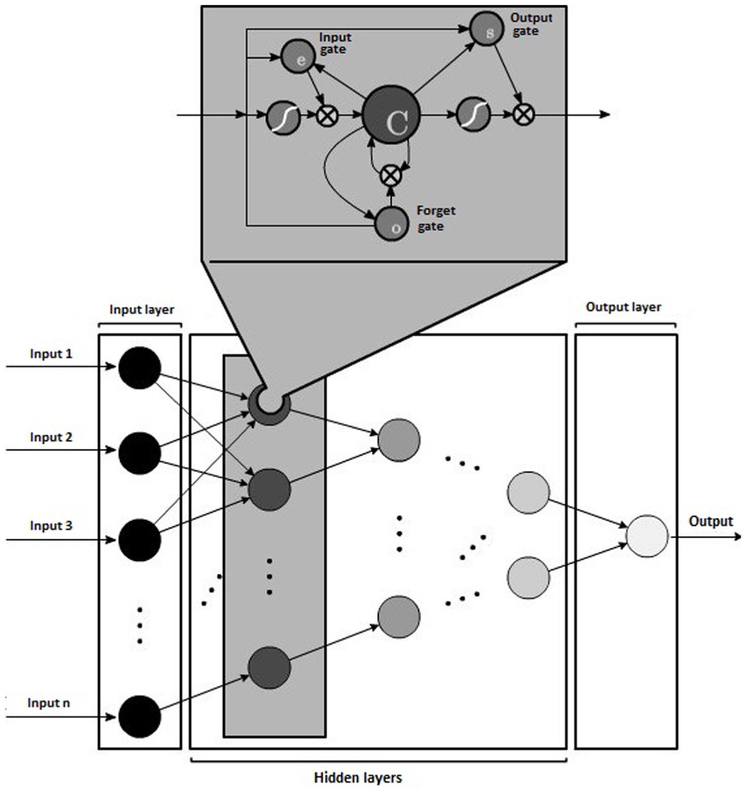
Graphical representation of LSTM-type neural networks.

Modeling of the input signal and LSTM model layers

A discrete input signal indicates the presence (1) or absence (0) of a PU within a spectrum band for a time period T, according to equation (1), in which, based on the binary sequence, the predictor is trained to forecast channel status not only in the next time slot, but also in subsequent points in time based on the historical data of a PU’s behavior in the channel

X_{0}^{T} = [x_{0}, x_{1}, x_{2}, x_{3}, \dots, x_{T}]

(1)

Determining the exact number of neurons for resolving the characterization problem is especially difficult. A very small neural network cannot learn how to correctly solve the problem, but a very large network will generate an over adjustment (i.e. the problem is singled out, not generalized).³² In addition, it must be taken into account that the more layers and neurons there are, the training time is greater, and more resources are used. In this article, the authors used a numerical optimization technique based on the geometric pyramid rule, which is especially useful when the number of input layer neurons is greater than the number of output layer neurons,³³ as is the case with this problem. Since it is necessary to divide the number of input layer neurons n times a power of $2$ until one is obtained, equation (2) is arrived at, where Co corresponds to the number of input layer neurons, and n to the number of existing layers

1 = \frac{Co}{2^{n}} \Rightarrow n = ⌈ lo g_{2} (Co) ⌉

(2)

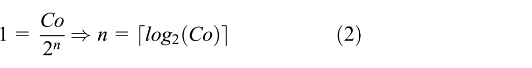
It is possible to discern from the preceding equation that the number of layers grows in a controlled fashion according to the increase in the number of input neurons. Due to the fact that a design decision was made to develop a dynamic software application where the creation of the LSTM neural network varies and depends on the input sequence, the total number of neurons that comprise a network topology is obtained from equation (3)

N = \sum_{i = 0}^{Co} ⌈ \frac{Co}{2^{i}} ⌉

(3)

Equation (3) can be approximated to a geometric series that converges to equation (4)

N \approx Co (2 - 2^{- Co})

(4)

Taking Co (from equation (4)) as a very large number, it can be assumed that the total number of neurons tends to

lim_{Co \to \infty} Co (2 - 2^{- Co}) = 2 Co = \infty

(5)

Equation (5) indicates that as the number of input layer neurons increases, the total number of neurons is approximately twice the number of input layer neurons.³⁴

LSTM system operating model

LSTM can be considered a differentiable function approximator that is usually trained with a descending gradient.³⁵ Although a truncated form of backpropagation through time (BPTT) was initially employed to approximate the error gradient,³⁶ a BPTT calculation without truncation, based on the discussion by Graves and Schmidhuber,³⁷ was used in this research. The operation of the LSTM neural network described in sections “Forward pass equations” and “Backward pass equations” uses the notation shown in Table 1.³⁵

Table 1.

Notation for the development of the mathematical model.

	Memory block	Input gate	Forget gate	Output gate	Memory cell
Subindex	i	l	$\emptyset$	w	c
Input	$x_{i}$	$a_{l}^{t}$	$a_{\emptyset}^{t}$	$a_{w}^{t}$	$a_{c}^{t}$ , $s_{c}^{t}$
Output	$y_{i}$	$b_{l}^{t}$	$b_{\emptyset}^{t}$	$b_{w}^{t}$	$b_{c}^{t} = b_{w}^{t} (s_{c}^{t})$
Number of units	I	N/A	N/A	N/A	C
Activation function	N/A	f Sigmoid function	f Sigmoid function	f Sigmoid function	f (in-cell)h (out-cell)

Forward pass equations

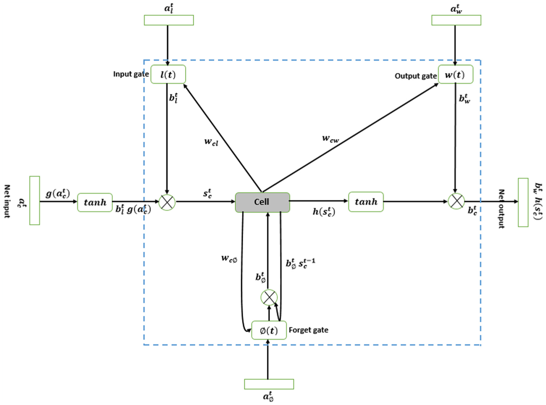
For the three cell gates (input, output, and forget),³⁵ the propagation functions $a_{l}^{t}$ , $a_{\emptyset}^{t}$ , and $a_{w}^{t}$ take into account not only the weighted sum of the current inputs, but also the outputs for the immediately preceding time for the blocks in the hidden layer and the status of other cells in the same block (except in the output gate where the current status of the cells is required). In this regard, equations (6) through (11)³⁵ result from the analysis of the LSTM block (Figure 3 modified from Palangi et al.³⁸) for each gate and memory cell comprising the model.

Figure 3.

LSTM architecture used for the characterization of PUs.

For the input gate

a_{l}^{t} = \sum_{i = 1}^{L} w_{il}^{t} x_{i}^{t} + \sum_{h = 1}^{H} w_{hl}^{t} b_{h}^{t - 1} + \sum_{c = 1}^{C} w_{cl} s_{c}^{t - 1} + θ_{l}

(6)

b_{l}^{t} = f (a_{l}^{t})

(7)

For the forget gate

a_{\emptyset}^{t} = \sum_{i = 1}^{L} w_{i \emptyset}^{t} x_{i}^{t} + \sum_{h = 1}^{H} w_{h \emptyset}^{t} b_{h}^{t - 1} + \sum_{c = 1}^{C} w_{c \emptyset} s_{c}^{t - 1} + θ_{\emptyset}

(8)

b_{\emptyset}^{t} = f (a_{\emptyset}^{t})

(9)

For the output gate

a_{w}^{t} = \sum_{i = 1}^{L} w_{iw}^{t} x_{i}^{t} + \sum_{h = 1}^{H} w_{hw}^{t} b_{h}^{t - 1} + \sum_{c = 1}^{C} w_{cw} s_{c}^{t - 1} + θ_{w}

(10)

b_{w}^{t} = f (a_{w}^{t})

(11)

In order to describe a cell’s behavior, two elements must be taken into account. The first one is the $a_{c}^{t}$ propagation function, which depends not only on current inputs, but also on outputs for the immediately preceding time from the other blocks in the hidden layer. The second one is the $s_{c}^{t}$ neuron status, which indicates if the neuron is keeping the information or will forget it, and depends on the outputs from the forget gate and the input gate.³⁴

The neuron output $b_{c}^{t}$ will indicate if new learning was generated or the stored information is kept. Now that the above is clear and based on Figure 3, it is concluded that cell status and output are given by equations (12)–(14).^34,35

Neuron status

a_{c}^{t} = \sum_{i = 1}^{L} w_{ic}^{t} x_{i}^{t} + \sum_{h = 1}^{H} w_{hc}^{t} b_{h}^{t - 1}

(12)

s_{c}^{t} = b_{\emptyset}^{t} s_{c}^{t - 1} + b_{l}^{t} g (a_{c}^{t})

(13)

Neuron output

b_{c}^{t} = b_{w}^{t} h (s_{c}^{t})

(14)

Backward pass equations

In order to obtain the backward pass equations, the BPTT method is used (as previously mentioned),³⁵ which implies using the chain rule to calculate the derivatives of errors at the exit of the components of an LSTM block.

When defining the outputs for input gate, output gate, and forget gate as $a_{j}^{t}$ , they can be represented as described in equation (15)³⁴

δ_{j}^{t} = \frac{\partial E}{\partial a_{j}^{t}}, where j \in {l, \emptyset, w}

(15)

In addition, in defining cell output ( $ε_{c}^{t}$ ) and cell status ( $s_{c}^{t}$ )

ϵ_{c}^{t} = \frac{\partial E}{\partial b_{c}^{t}}

(16)

ϵ_{s}^{t} = \frac{\partial E}{\partial s_{c}^{t}}

(17)

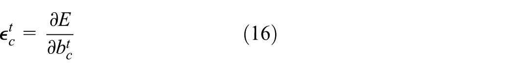
Defining E (in equations (16) and (17)) as the loss function (error), and based on the fact that the purpose is to establish how the error varies when the weights are modified, the following is obtained based on the chain rule

\frac{\partial E}{\partial w_{ij}} = \frac{\partial E}{\partial a_{j}} \frac{\partial a_{j}}{\partial w_{ij}} = b_{i} \frac{\partial E}{\partial a_{j}}

(18)

From equation (18), it is clear the goal is to calculate $\partial E / \partial a_{j}$ , but taking into account that in the case of LSTM, four types of a exist, namely ( $\partial E / \partial a_{w}^{t}$ ) output gate, ( $\partial E / \partial a_{c}^{t}$ ) cells, ( $\partial E / \partial a_{\emptyset}^{t}$ ) forget gate, and ( $\partial E / \partial a_{l}^{t}$ ) input gate, all of which can be defined as shown in equations (19)–(22)³⁴

\frac{\partial E}{\partial a_{w}^{t}} = \sum_{c = 1}^{C} \frac{\partial E}{\partial b_{c}^{t}} \frac{\partial b_{c}^{t}}{\partial b_{w}^{t}} \frac{\partial b_{w}^{t}}{\partial a_{w}^{t}} = \frac{\partial b_{w}^{t}}{\partial a_{w}^{t}} \sum_{c = 1}^{C} \frac{\partial E}{\partial b_{c}^{t}} \frac{\partial b_{c}^{t}}{\partial b_{w}^{t}}

(19)

\frac{\partial E}{\partial a_{c}^{t}} = \frac{\partial E}{\partial s_{c}^{t}} \frac{\partial s_{c}^{t}}{\partial a_{c}^{t}}

(20)

\frac{\partial E}{\partial a_{\emptyset}^{t}} = \sum_{c = 1}^{C} \frac{\partial E}{\partial s_{c}^{t}} \frac{\partial s_{c}^{t}}{\partial b_{\emptyset}^{t}} \frac{\partial b_{\emptyset}^{t}}{\partial a_{\emptyset}^{t}} = \frac{\partial b_{\emptyset}^{t}}{\partial a_{\emptyset}^{t}} \sum_{c = 1}^{C} \frac{\partial E}{\partial s_{c}^{t}} \frac{\partial s_{c}^{t}}{\partial b_{\emptyset}^{t}}

(21)

\frac{\partial E}{\partial a_{l}^{t}} = \sum_{c = 1}^{C} \frac{\partial E}{\partial s_{c}^{t}} \frac{\partial s_{c}^{t}}{\partial b_{l}^{t}} \frac{\partial b_{l}^{t}}{\partial a_{l}^{t}} = \frac{\partial b_{l}^{t}}{\partial a_{l}^{t}} \sum_{c = 1}^{C} \frac{\partial E}{\partial s_{c}^{t}} \frac{\partial s_{c}^{t}}{\partial b_{l}^{t}}

(22)

Taking into account that the summation is done over c because the model is developed in a single block (with C cells inside), the mathematical descriptions shown in equation (23) are found when calculating the respective derivatives³⁴

\begin{matrix} \frac{\partial s_{c}^{t}}{\partial b_{l}^{t}} = g (a_{c}^{t}) \frac{\partial s_{c}^{t}}{\partial b_{\emptyset}^{t}} = s_{c}^{t - 1} \frac{\partial b_{c}^{t}}{\partial b_{w}^{t}} = h (s_{c}^{t}) \\ \frac{\partial b_{\emptyset}^{t}}{\partial a_{\emptyset}^{t}} = f' (a_{\emptyset}^{t}) \frac{\partial s_{c}^{t}}{\partial a_{c}^{t}} = b_{l}^{t} g' (a_{c}^{t}) \frac{\partial b_{l}^{t}}{\partial a_{l}^{t}} = f' (a_{l}^{t}) \\ \frac{\partial b_{w}^{t}}{\partial a_{w}^{t}} = f' (a_{w}^{t}) \end{matrix}

(23)

Based on the mathematical analysis applied above, the following backward pass equations are obtained^34,35

Output gate

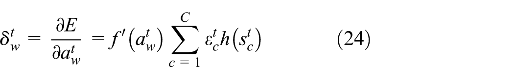
δ_{w}^{t} = \frac{\partial E}{\partial a_{w}^{t}} = f' (a_{w}^{t}) \sum_{c = 1}^{C} ε_{c}^{t} h (s_{c}^{t})

(24)

Cell

δ_{c}^{t} = \frac{\partial E}{\partial a_{c}^{t}} = ε_{s}^{t} b_{l}^{t} g' (a_{c}^{t})

(25)

Forget gate

δ_{\emptyset}^{t} = \frac{\partial E}{\partial a_{\emptyset}^{t}} = f' (a_{\emptyset}^{t}) \sum_{c = 1}^{C} ε_{s}^{t} s_{c}^{t - 1}

(26)

Input gate

δ_{l}^{t} = \frac{\partial E}{\partial a_{l}^{t}} = f' (a_{l}^{t}) \sum_{c = 1}^{C} ε_{s}^{t} g (a_{c}^{t})

(27)

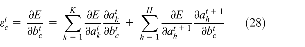
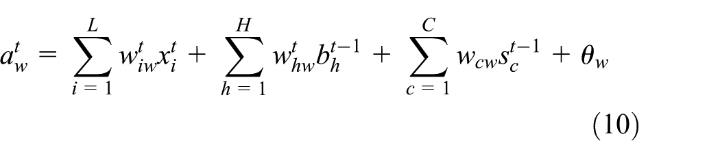
Note that equations (24)–(27) depend on the $ε_{s}^{t}$ and $ε_{c}^{t}$ terms; therefore, it is necessary to determine how the error is affected when making changes both to cell outputs and cell status.

In this case, keep in mind that the error is a function with variables that are the K outputs generated by the H blocks of the hidden layer; in fact, for a given block, the resulting output in a time t will affect the K units of the output layer (at a time t) and at the next input to each one of the H blocks in the hidden layer.³⁴ Therefore, $ε_{c}^{t}$ can be defined as

ε_{c}^{t} = \frac{\partial E}{\partial b_{c}^{t}} = \sum_{k = 1}^{K} \frac{\partial E}{\partial a_{k}^{t}} \frac{\partial a_{k}^{t}}{\partial b_{c}^{t}} + \sum_{h = 1}^{H} \frac{\partial E}{\partial a_{h}^{t + 1}} \frac{\partial a_{h}^{t + 1}}{\partial b_{c}^{t}}

(28)

The cell output is described as follows by equation (29)

ε_{c}^{t} = \sum_{k = 1}^{K} \frac{\partial E}{\partial a_{k}^{t}} w_{ck} + \sum_{h = 1}^{H} \frac{\partial E}{\partial a_{h}^{t + 1}} w_{ch}

(29)

Finally, it is necessary to analyze what happens with the error if changes to cell status are made. The status of the cell c in time $s_{c}^{t}$ indicates whether or not the information stored at the time was modified; therefore, $s_{c}^{t}$ is a value that affects the inputs of all gates, the next status of the cell and, obviously, the output of the cell. This is mathematically expressed in equation (30)³⁴

\begin{matrix} ε_{s}^{t} = \frac{\partial E}{\partial s_{c}^{t}} \\ = \frac{\partial E}{\partial b_{c}^{t}} \frac{\partial b_{c}^{t}}{\partial s_{c}^{t}} + \frac{\partial E}{\partial s_{c}^{t + 1}} \frac{\partial s_{c}^{t + 1}}{\partial s_{c}^{t}} + \frac{\partial E}{\partial a_{l}^{t + 1}} \frac{\partial a_{l}^{t + 1}}{\partial s_{c}^{t}} \\ + \frac{\partial E}{\partial a_{\emptyset}^{t + 1}} \frac{\partial a_{\emptyset}^{t + 1}}{\partial s_{c}^{t}} + \frac{\partial E}{\partial a_{w}^{t}} \frac{\partial a_{w}^{t}}{\partial s_{c}^{t}} \end{matrix}

(30)

The status of the cell is³⁵ (equation (31))

\begin{matrix} ε_{s}^{t} = ε_{c}^{t} \frac{\partial b_{c}^{t}}{\partial s_{c}^{t}} + ε_{s}^{t + 1} \frac{\partial s_{c}^{t + 1}}{\partial s_{c}^{t}} + δ_{l}^{t + 1} \frac{\partial a_{c}^{t + 1}}{\partial s_{c}^{t}} + δ_{\emptyset}^{t + 1} \frac{\partial a_{\emptyset}^{t + 1}}{\partial s_{c}^{t}} \\ + δ_{w}^{t + 1} \frac{\partial a_{w}^{t + 1}}{\partial s_{c}^{t}} \end{matrix}

(31)

Flowchart and pseudo-code for the LSTM system

The training flowchart (Figure 4) for the process begins by randomly initializing each neuron with values between −1 and 1; after that, each training example is read and the output is compared with the expected output. If the response obtained does not match what was expected, the algorithm calculates the error between the system output and the expected output, correcting each weight of the gates (input, output, forget) and the cell by applying weighting and making use of hyperbolic tangent and sigmoid functions until completing all training examples, thus bringing the model’s output close to the expected output (by error reduction, as shown in section “LSTM system operating model”).³⁴

Figure 4.

Flowchart for LSTM training.

Part of the pseudo-code for the algorithm that was implemented³⁴ is shown below.

LSTM algorithm
Data: The existence of a Wo, Wf, Wi and Wc array that represents the neural networkResult: A neural network trained with data from the training examplesforgetLayer = Wf.size(); //The size of the array representing the neural network is obtained.fori = 0; i < neurons; i++ do Wf[i] = random(-1,1); //Each layer of the neural network is initialized. Wi[i] = random(-1,1); Wc[i] = random(-1,1); Wo[i] = random(-1,1);endbf = 0.5; //Approximation of the output obtained for each layer.bc = 0.5;inputs = readInputs(); //Input examples are read.outputs = readOutputs(); //Output examples are read.size = inputs.size(); //The size of the examples is obtained.for i = 0; i < size; i++ do sumf = 0; for j = 0; j < neurons; j++ do sumf = sumf+Wf[j]inputs[i][j]; //The output for each example in each layer is calculated. sumi = sumi+Wi[j]inputs[i][j]; sumc = sumc+Wc[j]inputs[i][j]; sumo = sumo+Wo[j]inputs[i][j]; end ft = sigmoid(sumf+bf); //Approximations are made for each network output. it = sigmoid(sumi+bi); dct = tanh(sumc+bc); ct = ft+ itdct; ot = sigmoid(sumo+bo); output = ottanh(ct); //The neural network output is calculated. if output != outputs[i]then error = outputs[i]—output; forj = 0; j < neurons; j++ do Wo[j] = Wo[j]+inputs[i][j]*e; //Each neuron is traversed and the weighting is corrected with respect to the calculated error. end bo = 0.5+error; //The shift is corrected. end

LSTM algorithm

Data: The existence of a Wo, Wf, Wi and Wc array that represents the neural networkResult: A neural network trained with data from the training examplesforgetLayer = Wf.size(); //The size of the array representing the neural network is obtained.fori = 0; i < neurons; i++ do Wf[i] = random(-1,1); //Each layer of the neural network is initialized. Wi[i] = random(-1,1); Wc[i] = random(-1,1); Wo[i] = random(-1,1);endbf = 0.5; //Approximation of the output obtained for each layer.bc = 0.5;inputs = readInputs(); //Input examples are read.outputs = readOutputs(); //Output examples are read.size = inputs.size(); //The size of the examples is obtained.for i = 0; i < size; i++ do sumf = 0; for j = 0; j < neurons; j++ do sumf = sumf+Wf[j]*inputs[i][j]; //The output for each example in each layer is calculated. sumi = sumi+Wi[j]*inputs[i][j]; sumc = sumc+Wc[j]*inputs[i][j]; sumo = sumo+Wo[j]*inputs[i][j]; end ft = sigmoid(sumf+bf); //Approximations are made for each network output. it = sigmoid(sumi+bi); dct = tanh(sumc+bc); ct = ft+ it*dct; ot = sigmoid(sumo+bo); output = ot*tanh(ct); //The neural network output is calculated. if output != outputs[i]then error = outputs[i]—output; forj = 0; j < neurons; j++ do Wo[j] = Wo[j]+inputs[i][j]*e; //Each neuron is traversed and the weighting is corrected with respect to the calculated error. end bo = 0.5+error; //The shift is corrected. end

Results analysis and evaluation

Capture and processing of spectrum information

For data capture, the first step was to determine what wireless network application would be used to evaluate the deep learning–based technique.³⁶ Cellular (GSM) and Internet access (WiFi) communications were chosen as the main objective. The second step was to select the spectrum detection technique to be used. Energy detection was selected because it is easily implemented and has low requirements.³⁹ On the latter, it is important to indicate that in order to determine whether a frequency channel is occupied or not, a decision threshold was determined based on the noise floor average for the frequency band used, and from said value, a guard level of 5 dBm above was determined, with the aim of minimizing possible false alarms or detection failures.

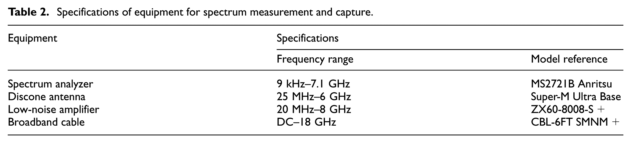
The manner in which data capture was performed is shown in Figure 5; Table 2 shows the spectrum measurement technical specifications. Table 3 shows the characteristics of the cluster used as a computing resource for the development of the algorithm and the execution of the training and prediction tests.

Figure 5.

Interconnection of equipment for capturing spectrum occupation data.³³

Table 2.

Specifications of equipment for spectrum measurement and capture.

Equipment	Specifications
	Frequency range	Model reference
Spectrum analyzer	9 kHz–7.1 GHz	MS2721B Anritsu
Discone antenna	25 MHz–6 GHz	Super-M Ultra Base
Low-noise amplifier	20 MHz–8 GHz	ZX60-8008-S+
Broadband cable	DC–18 GHz	CBL-6FT SMNM+

Table 3.

Cluster specifications.

Feature	Description
Equipment and brand	KVM Virtual Machine—BIOS OpenStack Foundation 2015.1
Brand	DELL R900 server
Number of processors	Intel(R) Xeon(R) CPU E7450 at 2.40 GHz, 24 Cores
RAM	64 GB DDR2
Storage system	1000 GB ext4
Operating system	Ubuntu server 14.04.04 with an XFCE4 desktop environment

For the processing of spectrum information, measurements were made every 290 ms in the WiFi band (2.4–2.48 GHz) and GSM (uplink 824–849 MHz) in terms of transmission power; in addition, in order to facilitate pattern recognition, power levels were presented in binary form based on the definition established in equation (32)³⁴

f (x) = {\begin{matrix} 0, if x ⩽ a \\ 1, if x > a \end{matrix}

(32)

where the values of a are −89 dBm for GSM and −88 dBm for WiFi.

Figure 6 shows the procedure for converting the spectrum data traces into discrete signals. It is worth noting that when performing the tests, a 6.79 GB database was available with information on GSM traffic traces, and a 9.63 GB database was available for WiFi traces, with more than 10,000 data records per files obtained from Pedraza et al.⁴⁰

Figure 6.

Flowchart for the discretization of spectrum data.

Evaluation and validation of the proposed LSTM algorithm

The performance of the proposed algorithm was tested for PU behavior with simulated and real data sequences (GSM and WiFi traces), based on the premise that 70% of the data is used in the LSTM network training stage, and the other 30% for validation (estimating the prediction).

First group of test cases

Behavior patterns (of multiple sizes) were created through simulation based on what is suggested in Saleem and Rehmani⁴¹ and in accordance with Table 4.³⁴

Table 4.

Test cases for PU traffic traces generated through simulation.

Identifier	Test case	Description
TC1	i % 2 === 0	Refers to historical data where all even-numbered time units show channel occupation
TC2	i % 5! === 0	Refers to historical data where all time units that are not a multiple of 5 show channeloccupation
TC3	i % 3 === 0	Refers to historical data where all time units that are a multiple of 3 show channeloccupation
TC4	i % 3 === 0 and i % 2 === 0	Refers to historical data where all time units that are a multiple of 3 and 2 show channeloccupation
TC5	Random	Refers to historical data where channel occupation is randomly generated

PU: primary user.

For qualitative purposes, results are presented for the LSTM algorithm when modeling and estimating the future behavior of a licensed user (for TC2), with a high fluctuation between presence and absence in the licensed channel.³⁵ The binary sequence that simulates channel use is made up of 50 digits. Figure 7 shows the sequence for the first 22 digits as 01111011110111101, where PU presence is represented by a 1, and PU absence, by a 0.

Figure 7.

Behavior of historical data for 77 samples.

The application that was developed generates adaptively (Figure 8) the LSTM neural network structure that is most appropriate for the input sequence according to what was set forth in section called “Modeling of the input signal and LSTM model layers.”

Figure 8.

Neural network topology.

The learning stage (training-modeling) is shown in Figure 9, where it is concluded that the LSTM network was 100% capable of determining the pattern of channel use.

Figure 9.

Results of the training stage (network learning phase).

The future estimation (forecast) delivered by the neural network through the developed application is shown in Figure 10, where we can see that the success level comparing the original signal (purple sequence) and the one projected by the system (blue lines) is 81.77%, concluding that the prediction error is 18.2275%, which indicates that the network is relatively efficient for the case evaluated. Quantitative results for the different cases listed in Table 4 are shown in Table 5. The performance evaluation metrics (Table 5) refer to average values, because historical data of various sizes were created (17, 35, 77, 157, and 200 binary digits), applying 10 tests for each case because different solutions could be obtained each time the algorithm is executed. The LSTM algorithm was validated with the same metrics and the same considerations, but using a pyramid MLPNN (see Table 6).

Figure 10.

Prediction results.

Table 5.

Performance of LSTM in the characterization of PUs.

LSTM
Test case	Average validation error (%)	Average prediction error (%)	Number of iterations	Processing time (ms)
TC1	0.0753007	0	1222	50.3
TC2	0.0881980	18.2275399	1301	72.1
TC3	0.7995310	25.9980047	4971	498.0
TC4	0.7100676	13.7908176	3411	799.7
TC5	0.7377944	35.4555091	1655	6341

LSTM: long short-term memory; PU: primary user.

Table 6.

Performance of MLPNN in the characterization of PUs.

MLPNN
Test case	Average validation error (%)	Average prediction error (%)	Number of iterations	Processing time (ms)
TC1	0.03372774	0	1431	75.80
TC2	0.05700592	22.5366130	4114	239.5
TC3	0.10012006	34.0007921	5200	513.4
TC4	0.83274439	18.1117448	4355	940.6
TC5	0.47006433	50.8190674	4939	2002.

MLPNN: multilayer perceptron neural network; PU: primary user.

Analysis of Tables 5 and 6 reveals that the average prediction error for LSTM ranges from 0% to 35.45%, placing the forecast level above 64.54% in the worst case (TC5), a percentage that is higher than what was found with MLPNN (49.19%). This indicates LSTM was able to generalize the behavior for the various cases that were submitted and was able to adequately predict PU behavior at any instant in time t as long as the PU continues to have the same behavior. Another important feature is that although LSTM has more neurons in its structure than MLPNN, it required less iterations in TC1 through TC4, which proves that the complexity of the LSTM structure allows abstracting the PU signal behavior pattern at a lower computing cost when the size of the matrix used for historical data has a short length. Finally, the average validation error is very small for both types of neural networks, a condition that guarantees the network can be optimally modeled.

Second group of test cases

To demonstrate the viability of the proposed algorithm with real GSM and WiFi traffic traces (according to the characteristics laid out in section “Capture and processing of spectrum information”), a metric called Index of Occupation (Io) was defined (equation (33)) in order to divide spectrum band use levels into high, medium, and low; this allows a more objective and detailed assessment

I o = \frac{\sum_{x = 0}^{n} t (x)}{n} 100 %

(33)

where $t (x)$ corresponds to discretized data flows, and n is the number of elements at t(x). The resulting outputs are summarized in Tables 7 and 8. For reference, a trace with 18,000 data was used to feed the system for each one of the three frequency bands selected (according to their occupation index), and 10 tests were executed in each case.

Table 7.

Algorithm performance for GSM flows.

Metric	LSTM		MLPNN		Bayesian networks		ANFIS-Grid
Metric	High index	Low index	High index	Low index	High index	Low index	High index	Low index
Number of iterations	4.000	4.000	4.000	4.000	4.000	4.000	4.000	4.000
Training error	0.4728	0.0889	0.4932	0.1201	0.4554	0.1132	0.4785	0.0898
Processing time (ms)	7322987	7227001	1599510	1409976	3571754	3499812	5991919	5771509
Validation error (%)	18.44	1.850	19.97	2.679	20.01	2.30	19.37	2.75
Prediction error (%)	20.15	1.750	23.11	2.875	22.15	2.394	21.88	1.97

LSTM: long short-term memory; MLPNN: multilayer perceptron neural network; ANFIS-Grid: adaptive neuro-fuzzy inference systems.

Table 8.

Algorithm execution results for WiFi flows.

Metric	LSTM		MLPNN		Bayesian networks		ANFIS-Grid
Metric	High index	Low index	High index	Low index	High index	Low index	High index	Low index
Number of iterations	4.000	4.000	4.000	4.000	4.000	4.000	4.000	4.000
Training error	0.7322	0.3401	0.7439	0.3777	0.7395	0.3697	0.7878	0.3500
Processing time (ms)	6911211	7002789	1200787	1149090	3122432	30903767	5503862	5487611
Validation error (%)	28.74	10.75	29.94	9.870	21.00	12.46	29.02	10.98
Prediction error (%)	35.13	12.54	38.22	15.36	36.75	13.11	36.10	12.97

LSTM: long short-term memory; MLPNN: multilayer perceptron neural network; ANFIS-Grid: adaptive neuro-fuzzy inference systems.

Based on the quantitative results in the above tables, it can initially be concluded that the training time of the various models for estimating channel use behavior (on the part of PUs) is greater in the case of LSTM due to greater complexity (input, output, and forget cells) incurred by this type of recurrent network when modeling PUs. LSTM’s ability to learn patterns and forget sequences directly impacts the validation error performance evaluation metric, which is optimal in comparison with MLPNN, Bayesian networks, and ANFIS-Grid. It was also found that the training error exhibits better values in LSTM than in ANFIS-Grid, due to its storage and pattern utilization capability over time, a characteristic that is inherent to deep learning intelligent systems.

Regarding LSTM’s accuracy percentage, the values range between 98.25% (for a low Io) and 79.85% (for a high Io) in GSM systems, and between 87.46% (for a low Io) and 64.87% (for a high Io) in WiFi, thus validating that LSTM is more efficient than MLPNN, Bayesian networks, and ANFIS-Grid, as shown in Table 9; however, it is important to point out that greater efficiency implies greater hardware requirements, a factor that is not relevant if the prediction system is implemented in CR networks with a centralized topology.

Table 9.

Accuracy percentage in the estimation of licensed channel use by primary users.

Evaluation algorithm	LSTM		MLPNN		Bayesian networks		ANFIS-Grid
Evaluation algorithm	High index	Low index	High index	Low index	High index	Low index	High index	Low index
GSM
Estimation accuracypercentage (%)	79.85	98.25	76.89	97.12	77.85	97.60	78.12	98.03
WiFi
Estimation accuracypercentage (%)	64.87	87.46	61.78	84.64	63.25	86.89	63.90	87.03

LSTM: long short-term memory; MLPNN: multilayer perceptron neural network; ANFIS-Grid: adaptive neuro-fuzzy inference systems.

Regarding the algorithms’ performance improvement with GSM and WiFi traffic traces, better performance is observed for GSM, probably due to the chaotic nature of signals in WiFi networks.

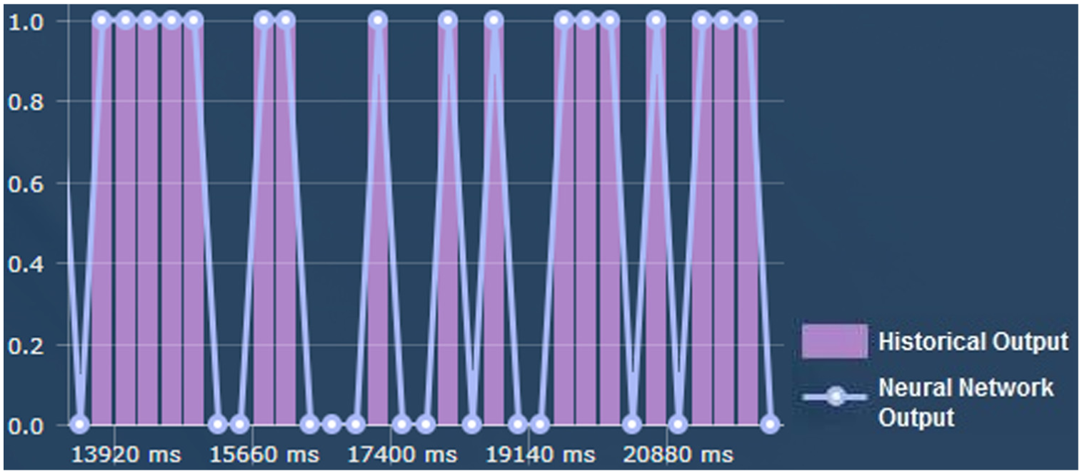
Finally, just as in the first test case, Figures 11 –14 are a qualitative description of the visual behavior of the characterization software that was developed, in part of the sequence used as a historical representation in system performance evaluation with GSM traces.

Figure 11.

Historical representation of inputs to the system (discretized GSM traces).

Figure 12.

LSTM network topology dynamically generated by software.

Figure 13.

Results of the training stage (network learning phase).

Figure 14.

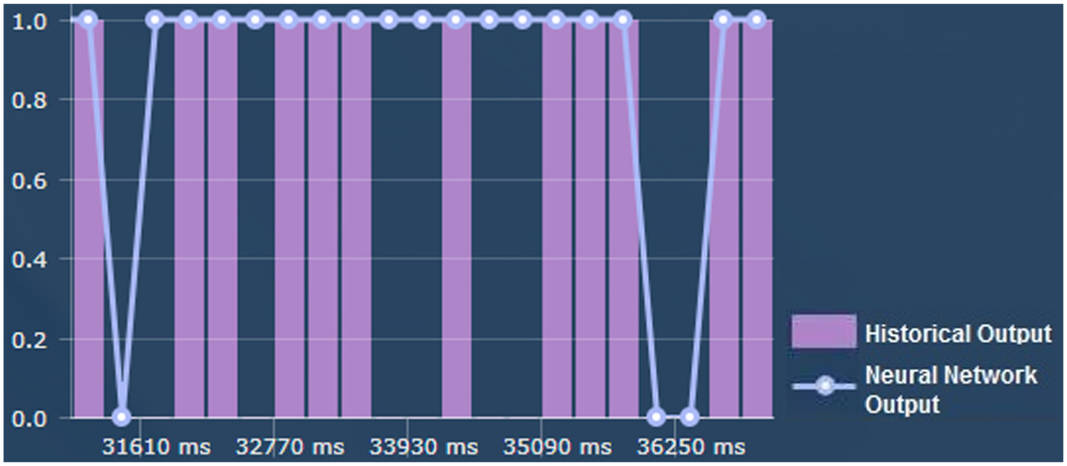
Prediction delivered by the characterization software with LSTM.

Discussion

In the AI field, neural networks have been extensively applied to time series given the prediction capabilities for unknown time units, due to the ability to be trained by means of examples in order to abstract a behavior. This contrasts with other AI techniques, which obtain the knowledge from an expert through the representation of variables relevant to the solution of the problem. One of the most widely used supervised learning methodologies for the characterization of PUs is MLPNN, which can achieve an efficiency improvement of up to 60% in prediction, as concluded in Adeel et al.⁴² (although higher percentages were achieved in tests); however, there have been recent proposals for the use of techniques based on deep learning, due to its high abstraction level⁴³ for the solution of multiple problems,^44–47 a significant reason for suggesting its use in CR.

From the analysis in the previous section, it is evident that although LSTM exhibits a greater prediction capability, it still has a significant estimation error in cases in which PU behavior is chaotic or random; however, obtaining an error close to zero is difficult due to signal nature, a condition that can be supported from the perspective of entropy. From equation (34), when entropy is 1, this indicates there is a 50% probability the spectrum band is occupied at any point in time, which generates a high level of uncertainty when making channel occupation estimations. The opposite occurs when the value tends to zero (a more favorable condition)

E_{s} = \sum_{i = 0}^{n} p (x_{i}) * lo g_{2} (\frac{1}{p_{x_{i}}})

(34)

where $p (x_{i})$ refers to the probability of appearance of the character $x_{i}$ and n to the number of characters.

Based on the above consideration, when calculating, for example, values for GSM–LSTM with high and low occupation indices, values of 0.7087981 and 0.1589255, respectively, are obtained, which is coherent with the prediction errors in Table 7; on the other hand, historical data generate indications of PU behavior, but no guarantee that it will actually occur again. However, having an indication of possible behavior allows a cognitive network central station to be prepared to take actions on the possible assignment of a frequency band to a SU.

An additional contribution of the application that was developed (for the LSTM algorithm) is the ability to automatically create a neural structure according to the size of the trace to be characterized; this is positive because no additional efforts are required to build the topology when modifying the behavior of input data. The opposite occurs, for example, in Adeel et al.⁴² and Winston et al.⁴⁸

Another important aspect of analyzing relates to the speed of convergence shown by the algorithms (Figures 15 and 16), where it can be seen that the convergence time of LSTM is 78.15% (in the case of GSM) and 82.62% (in the case of WiFi) slower than MLPNN; this is due to the ability of LSTM to detect, process, and memorize characteristic patterns in PU signals that can later be reused to raise the level of prediction; this allows to infer that although LSTM improves the characterization of PUs, the computational cost is much higher since the operational complexity (described in Figure 3) is much greater.

Figure 15.

Convergence time for GSM traffic flows.

Figure 16.

Convergence time for WiFi traffic flows.

Finally, based on the results of PU activity modeling with the LSTM methodology, and taking as reference the proposal’s validation with respect to the MLPNN, Bayesian network, and ANFIS-Grid learning techniques, it can be concluded that deep learning–based techniques are potentially more suitable for solving the current problem in CRN networks. The reason is the structures contain deep layers or processing units that specialize in the detection of certain characteristics or hidden patterns in processed data, which are not found in other types of networks such as the ones evaluated in this article.

Conclusion and future work

Given the research results, the proposal for developing PU characterization algorithms that operate on input data using neural networks^49,50 based on deep learning (as is the case for LSTM) should be considered a real and valid option in the search for new methodologies to minimize modeling and prediction error in the estimation of spectrum band use by PUs, thus improving performance in the spectrum decision stage for CR wireless networks. This statement is supported by the validation of results obtained with LSTM in contrast with other neural network techniques such as MLPNN, Bayesian networks, and ANFIS-Grid.

In reference to the test cases, where various PU behaviors were simulated, it was found that LSTM can easily adapt to multiple variations in traffic patterns, with a forecast accuracy above 79%; when the historical sequence has a prolonged absence/presence characteristic (as in television signals), it is possible to find estimations above 82%.

An important aspect of the research (contrary to what is said in multiple state-of-the-art proposals) is that the operation of the algorithm was corroborated with real traffic sources (GSM and WiFi), achieving accuracy percentages ranging from 79.85% to 98.25% (for GSM), thus proving the use of LSTM in real wireless systems is promising.

Based on multiple existing characterization proposals, there is no doubt that the application of LSTM neural networks is an innovative concept for the solution of the modeling and prediction problem. This line of research should continue to be evaluated when, for example, the neural system input data sequence does not exhibit a binary behavior, but a continuous behavior. The response to methodologies based on Arima time series should also be validated.

Footnotes

Handling Editor: Michelangelo Ceci

Declaration of conflicting interests

The author(s) declared no potential conflicts of interest with respect to the research, authorship, and/or publication of this article.

Funding

The author(s) received no financial support for the research, authorship, and/or publication of this article.

ORCID iD

Danilo López

References

Shared Spectrum Company. Spectrum reports: spectrum occupancy measurement. General survey of radio frequency bands (30 MHz to 3 GHz): Vienna, Virginia, http://www.sharedspectrum.com/papers/spectrum-reports/ (accessed 7 June 2015).

Federal Communications Commission. Notice of proposed rulemaking and order, Mexico D.F. Report ET Docket No. 03-332, September 2003.

IEEE Standard 1900.1:2008. IEEE Standard definitions and concepts for dynamic spectrum access: terminology relating to emerging wireless network, system functionality and spectrum management.

Sahai

Hoven

Tandra

Some fundamental limits on cognitive radio. Department of Electrical Engineering and Computer Science, University of California, http://www.eecs.berkeley.edu/∼sahai/Papers/cognitive_radio_preliminary.pdf (accessed 17 January 2015).

Fortuna

Mohorcic

Trends in the development of communication networks: cognitive networks. J Comput Netw 2009; 53: 1354–1376.

Popescu

Yao

Fiedler

et al . A management architecture for multimedia communication in cognitive radio networks. In: Hu

Kumar

(eds) Multimedia over cognitive radio networks. London: CRC Press, 2014, pp.3–25.

Masonta

Mzyece

Ntlatlapa

Spectrum decision in cognitive radio networks: a survey. Commun Surv Tut 2013; 15: 1088–1107.

Khalid

Anpalagan

Emerging cognitive radio technology: principles, challenges and opportunities. Comput Electr Eng 2010; 38: 358–366.

Akyildiz

Lee

W-Y

Chowdhury

Spectrum management in cognitive radio ad hoc networks. IEEE Netw 2009; 23: 6–12.

10.

Akyildiz

Lee

W-Y

Chowdhury

CRAHNS: cognitive radio ad hoc networks. Ad Hoc Netw 2009; 7: 810–836.

11.

López

Trujillo

Gualdron

Elementos fundamentales que componen la radio cognitiva y asignación de bandas espectrales. Inform Tecnol 2015; 26: 23–40.

12.

Wang

Guo

et al . Earthquake prediction based on spatio-temporal data mining: an LSTM network approach. IEEE T Emerg Top Comput 2017; 1–10. DOI: 10.1109/TETC.2017.2699169.

13.

Cheng

Liu

. Mechanical state prediction based on LSTM neural network. In: Proceedings of the 36th Chinese control conference, Dalian, China, 26–28 July 2017. New York: IEEE.

14.

Zhou

Luo

Modified primal-dual neural networks for motion control of redundant manipulators with dynamic rejection of harmonic noises. IEEE T Neur Net Lear 2018; 29: 4791–4801.

15.

Jin

Luo

et al . Neural dynamics for cooperative control of redundant robot manipulators. IEEE T Ind Inform 2018; 14: 3812–3821.

16.

Ceci

Corizzo

Fumarola

et al . Predictive modeling of PV energy production: how to set up the learning task for a better prediction?IEEE T Ind Inform 2017; 13: 956–966.

17.

Mishra

Tong

Chan

et al . Energy aware spectrum decision framework for cognitive radio networks. In: Proceedings of the international symposium electronic system design, Kolkata, India, 19–22 December 2012. New York: IEEE.

18.

Uyanik

Canberk

Oktug

Predictive spectrum decision mechanisms in cognitive radio networks. In: Proceedings of the Globecom workshop, Anaheim, CA, 3–7 December 2012. New York: IEEE.

19.

Bouali

Contribution to spectrum management in cognitive radio networks: a cognitive management framework. Doctoral Dissertation, Universitat Politècnica de Catalunya, Barcelona, 2013.

20.

Khan

Decision making techniques for cognitive radios. MSc Thesis, Blekinge Institute of Technology, Karlskrona, 2008.

21.

Chen

Iellamo

Coupechoux

et al . Spectrum auction with interference constraint for cognitive radio networks with multiple primary and secondary users. J Wirel Netw 2011; 17: 1355–1377.

22.

Canberk

Akyildiz

Oktug

. A QoS-aware framework for available spectrum characterization and decision in cognitive radio networks. In: Proceedings of the international symposium on personal indoor and mobile radio communications, Istanbul, Turkey, 26–30 September 2010. New York: IEEE.

23.

López

Hernández

Trujillo

SVM and ANFIS as channel selection models for the spectrum decision stage in cognitive radio network. J Contemp Eng Sci 2017; 10: 475–502.

24.

Xing

Jing

Huo

et al . Channel quality prediction based on Bayesian inference in cognitive radio networks. In: Proceedings of the international conference on computer communications, Turin, 14–19 April 2013. New York: IEEE.

25.

Butun

Talay

Altilar

et al . Impact of mobility prediction on the performance of cognitive radio networks. In: Proceedings of the wireless telecommunications symposium, Tampa, FL, 21–23 April 2010. New York: IEEE.

26.

Yao

Ngoga

Popescu

. Cognitive radio spectrum decision based on channel usage prediction. In: Proceedings of the 8th Euro-NF conference on next generation Internet, Karlskrona, 25–27 June 2012. New York: IEEE.

27.

Graves

Mohamed

Hinton

Speech recognition with deep recurrent neural network. In: Proceedings of the international conference on acoustics speech and signal processing, Vancouver, BC, Canada, 23–26 May 2013. New York: IEEE.

28.

Salgado

Algoritmo multivariable para la selección dinámica del canal de backup en redes de radio cognitiva basado en el método fuzzy analitical hierarchical process. Bogotá, Colombia: Faculty of Engineering, Francisco José de Caldas District University, 2014.

29.

Bae

Newman

et al . A survey of artificial intelligence for cognitive radios. IEEE T Veh Technol 2010; 59: 1578–1592.

30.

Veeriah

Zhuang

-J. Differential recurrent neural networks for action recognition. In: Proceedings of the international conference on computer vision, Santiago, Chile, 7–13 December 2015. New York: IEEE.

31.

Artiemjew

Jiao

Data mining and machine learning. In: Yao

et al . (eds) Rough sets, fuzzy sets, data mining and granular computing. Tianjin, China: Springer, 2015, pp.267–280.

32.

Kwok

T-Y

Yeung

D-Y.

Constructive algorithms for structure learning in feedforward neural networks for regression problems. IEEE T Neur Net Lear 1997; 8: 630–645.

33.

Masters

Multilayer feedforward networks. In: Timothy Masters (ed.) Practical neural network recipes in C++. San Diego, CA: Academic Press, 1993, pp.77–116.

34.

López

Rivas

Gualdron

Primary user characterization for cognitive radio wireless networks using a neural system based on deep learning. J Artif Intel Rev 2017; 1–27. DOI: 10.1007/s10462-017-9600-4.

35.

Graves

Supervised sequence labelling with recurrent neural networks. Berlin: Springer, 2012, pp.37–93.

36.

Schmidhuber

Long short-term memory. J Neur Comput 1997; 9: 1735–1780.

37.

Graves

Schmidhuber

Framewise phoneme classification with bidirectional LSTM and other neural network architectures. In: Proceedings of the international joint conference on neural network, Montreal, QC, Canada, 31 June–4 August 2005. New York: IEEE.

38.

Palangi

Ward

Deng

Distributed compressive sensing: a deep learning approach. Cornell University Library, https://arxiv.org/abs/1508.04924 (accessed 17 September 2015).

39.

Hernández

Salgado

López

et al . Multivariable algorithm for dynamic channel selection in cognitive radio networks. EURASIP J Wirel Commun Netw 2015; 2015(1): 1–17.

40.

Pedraza

Hernández

Galeano

et al . Ocupación espectral y modelo de radio cognitiva para Bogotá. Bogotá, Colombia: Francisco José de Caldas District University (UD Editorial), 2016.

41.

Saleem

Rehmani

Primary radio user activity models for cognitive radio networks: a survey. J Netw Comput Appl 2014; 43: 1–16.

42.

Adeel

Larijani

Ahmadinia

. Performance analysis of artificial neural network-based learning schemes for cognitive radio systems in LTE-UL. In: Proceedings of the 28th international conference on advanced information networking and applications workshops, Victoria, BC, Canada, 13–16 May 2014. New York: IEEE.

43.

Kalkan

Special topics in deep learning. Ankara, Turkey: Middle East Technical University, 2015.

44.

Sun

Feng

Chen

et al . A deep learning framework of quantized compressed sensing for wireless neural recording. J IEEE Access 2016; 4: 5169–5178.

45.

Palangi

Deng

Shen

et al . Deep sentence embedding using long short-term memory networks: analysis and application to information retrieval. IEEE T Audio Speech Process 2016; 24: 694–707.

46.

Sundermeyer

Ney

Schlüter

From feedforward to recurrent LSTM neural networks for language modeling. IEEE T Audio Speech Process 2015; 23: 517–529.

47.

Gers

Schmidhuber

LSTM recurrent networks learn simple context-free and context-sensitive languages. IEEE T Neur Net Lear 2001; 12: 1333–1340.

48.

Winston

Thomas

OkelloOdongo

. Optimizing neural network for TV Idle channel prediction in cognitive radio using particle swarm optimization. In: Proceedings of the 5th international conference on computational intelligence, communication systems and networks, Madrid, 5–7 June 2014. New York: IEEE.

49.

López

Ordoñez

Trujillo

User characterization through dynamic Bayesian networks in cognitive radio wireless networks. Int J Eng Technol 2016; 8: 1771–1783.

50.

López

Anzola

Zapata

et al . Designing a MAC algorithm for equitable spectrum allocation in cognitive radio wireless networks. J Wirel Pers Commun 2018; 98: 363–394.

Primary user characterization for cognitive radio wireless networks using long short-term memory

Abstract

Keywords

Introduction

Scientific review

Development of the proposal

LSTM

Modeling of the input signal and LSTM model layers

LSTM system operating model

Forward pass equations

Backward pass equations

Flowchart and pseudo-code for the LSTM system

Results analysis and evaluation

Capture and processing of spectrum information

Evaluation and validation of the proposed LSTM algorithm

First group of test cases

Second group of test cases

Discussion

Conclusion and future work

Footnotes

Declaration of conflicting interests

Funding

ORCID iD

References