Sage Journals: Discover world-class research

Abstract

Tuning the parameters of Computerized Numerical Control (CNC) is essential for practical manufacturers. Well configured parameters ensure the efficiency of production and the accuracy of the products. However, with the abrasive wear on the flank of the milling cutter, the milling processing parameters should re-configure to adapt to the increment of the abrasive wear. This paper aims to propose a method to predict the abrasive wear rate increment on the flank of the milling cutter and optimize the processing parameters of CNC milling. Firstly, we set a cutting data acquisition system to sample the processing time and cutting force among X, Y coordinates based on the five-factor and four-level orthogonal experiments. Then, the sampled cutting force data increment is transformed into the abrasive wear rate increment by applying the incremental model. Next, five processing parameters for CNC milling are optimized by the gray relational method, which takes the limited abrasive wear rate increment of the flank face and the non-increasing processing time as the constrained conditions. We obtain the relationship between five processing parameters and abrasive wear rate increment. We also find the basic principle of selecting process parameters is to reduce the abrasive wear rate without increasing the processing time. The experimental results verify that the optimized process parameters make the gray relational degree increase by 0.02, and the abrasive wear rate increment decreases by 0.42432 × 10⁻¹⁰ mm³/s without affecting the production efficiency. In the prediction section, by applying the Back Propagation (BP) neural network, we obtain an accurate prediction model from measurable five factors to the abrasive wear increment on the flank of the milling cutter. The maximum error between the predicted value and the actual value is 0.0003, and the predicted value curve fits well with the actual value curve. From the perspective of abrasive wear rate increment prediction, it provides a new idea for online tool wear monitoring.

Keywords

Abrasive wear rate increment gray relational method parameter optimization BP neural network increment prediction

Introduction

In CNC milling, selecting proper milling process parameters and predicting milling cutter wear are all fundamentals to ensure product processing accuracy, prevent processed parts from being scrapped, improve production efficiency, and reduce production costs. Many researchers made some progress in parameter optimization, and prediction of milling cutter wear in recent years.

In terms of optimization of milling process parameters: Li et al.¹ propose the cutting parameters optimization technology by combining the response surface methodology with the improved teaching learning based optimization algorithm. It is to obtain the best cutting parameters under multi-objective conditions. Shi et al.² introduce Taguchi with gray relational analysis of experimental data to determine an optimum combination of process parameters for promoting the surface roughness and the micro hardness of dry milling magnesium alloy. Du et al.³ investigate the optimization of high-speed milling process parameters for the new ultra high strength titanium alloy TB17, based on multiple performance characteristics. Tong et al.⁴ state the optimal mesoscopic geometric characteristic parameters under the four evaluation indices, such as mechanical thermal characteristics, tool wear, and surface quality of the workpiece. Shang et al.⁵ propose a reliability optimization model of milling process parameters considering the variations of milling speeds and feeds per tooth. Sarıkaya et al.⁶ optimize the milling characteristics with mono and multiple response outputs such as vibration signals, cutting force, and surface roughness.

Amount of optimization of milling process parameters, most studies focus on material removal rate, surface roughness, cutting force, cutting heat, vibration, or other factors. The abrasive wear rate increment is rarely applied to tune the parameters of CNC milling.

In this paper, the abrasive wear rate increment and material removal rate are used to optimize the CNC milling process parameters.

In terms of prediction of milling cutter wear: Zhang et al.⁷ introduce a tool wear prediction model with cutting parameters and cutting time. Chen et al.⁸ propose and evaluate an artificial neural networks based in process tool wear prediction system. Dai et al.⁹ improve the prediction accuracy and generalization performance of tool wear monitoring based on deep learning. Ding et al.¹⁰ state a novel method for tool wear prediction in titanium milling using the Simulink feedback method. Cao et al.¹¹ introduce a tool condition monitoring approach based on a convolutional neural network. Cus et al.¹² and Wang and Wang¹³ study the relationship between tool wear and cutting force. Signal analysis technology combined with artificial intelligence technology was used to extract the relevant features of cutting force, then the tool wear status was predicted. The development of artificial intelligence technology provides effective means for the analysis of tool wear. Since the increment of tool wear is considered as the object, we take the cutting force for the object instead. In this paper, the cutting force is obtained through the experimental method. The increment of cutting force is transformed into the increment of abrasive wear rate to characterize the tool wear state. The Back Propagation (BP) neural network technology is used to predict the increment of abrasive wear rate of the flank face of the cutting tool.

Milling experiment

Experiment design

This experiment uses Donghua DH5922D as the cutting data acquisition system. We also use an XD20 vertical milling machine, high-speed steel cutter. The material used in this study is 2A12 aluminum alloy, the length is 120 mm, the width is 50 mm, and the thickness is 40 mm. The cutting method is down-milling. The material removal amount is limited to 10,000 mm³. The cutting data acquisition system is shown in Figure 1:

Figure 1.

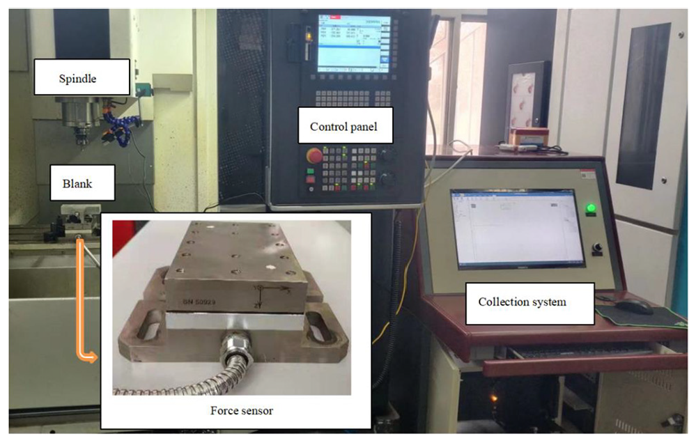
Cutting data acquisition system.

The orthogonal experiment factors and levels are shown in Table 1. Ф means tool diameter, unit mm. s means spindle speed, unit rpm. f means feed speed, unit mm/min. a_p means axial depth of cut, unit mm. a_e means radial depth of cut, unit mm.

Table 1.

Orthogonal experiment factors, level table.

Level	Factors
	Ф	s	f	a _p	a _e
1	6	1800	460	6	1
2	8	2000	480	8	1.5
3	10	2200	500	10	2
4	12	2400	520	12	2.5

The number of orthogonal experiments designed according to four levels and five factors is 16, the orthogonal experiment table is shown in Table 2:

Table 2.

Orthogonal experiment table.

Group no.	Ф	s	f	a _p	a _e
1	6	1800	460	6	1
2	6	2000	480	8	1.5
3	6	2200	500	10	2
4	6	2400	520	12	2.5
5	8	1800	480	10	2.5
6	8	2000	460	12	2
7	8	2200	520	6	1.5
8	8	2400	500	8	1
9	10	1800	500	12	1.5
10	10	2000	520	10	1
11	10	2200	460	8	2.5
12	10	2400	480	6	2
13	12	1800	520	8	2
14	12	2000	500	6	2.5
15	12	2200	480	12	1
16	12	2400	460	10	1.5

Data collection

The Donghua DH5922D cutting data acquisition system is used to obtain the total processing time when the material removal is 10,000 mm³. And, we can get the cutting force in the X and Y directions.

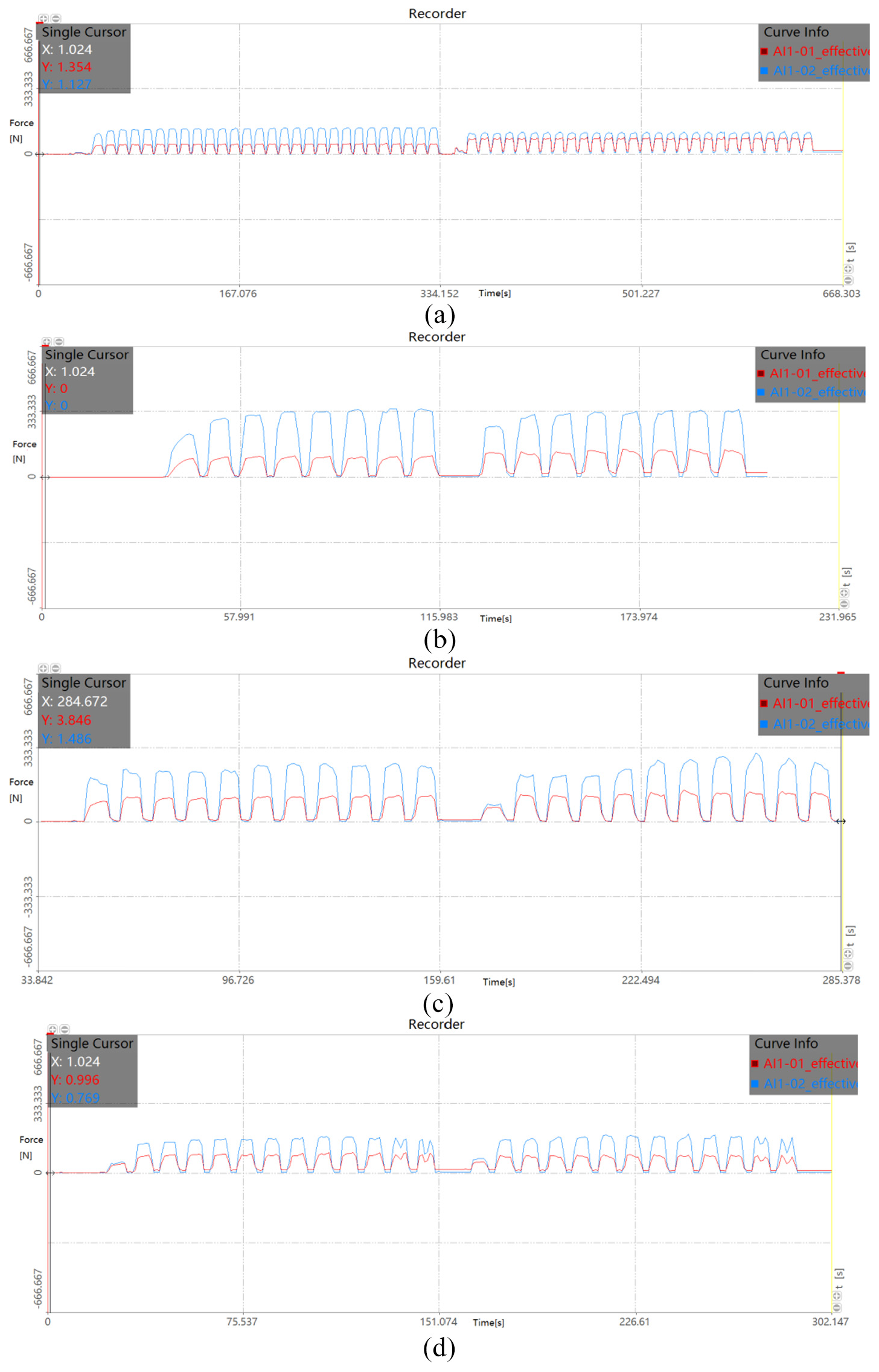
The cutting force in the X and Y directions is shown in Figure 2. Due to space limitation, only the cutting force diagrams of the 1, 5, 9, and 13 experiments are listed here. Red represents the cutting force in the X direction, blue is the cutting force in the Y direction. The directions of the tool force are opposite to the directions shown in the schematic diagram of the force sensor in Figure 2.

Figure 2.

Two-way cutting force diagram: (a) Group 1 experiment cutting force, (b) Group 5 experiment cutting force, (c) Group 9 experiment cutting force, and (d) Group 13 experiment cutting force.

The abscissa represents the processing time, s and the ordinate represents cutting force, N.

Continuously count the data of 1024 points, the root mean of the square is taken to obtain a smooth curve of cutting force, red represents a cutting force in the X direction, blue is cutting force in the Y direction. As shown in Figure 3.

Figure 3.

Root mean square graph of two-way cutting force: (a) root mean square curve of cutting force in group 1, (b) root mean square curve of cutting force in group 5, (c) root mean square curve of cutting force in group 9, and (d) root mean square curve of cutting force in group 13.

Abscissa represents the processing time, s and ordinate represents root mean square cutting force, N.

Since the cutting method is down-milling and the irregular shape of the blank will have an unstable impact on the tool force, the force of the first tool path and the last tool path is ignored. The average force of the first 2–4 tool path is taken as the force of the tool when removing the first 5000 mm³ material and the average force of the last 2–4 tool path is taken as the force of the tool when the remaining 5000 mm³ material is removed. F_x₁ represents the force applied to the tool in X direction when the first 5000 mm³ material is removed, N. F_x₂ represents the force applied to the tool in X direction when the remaining 5000 mm³ material is removed, N. ΔF_x represents the tool force increment in X direction. F_y₁ represents the force applied to the tool in Y direction when the first 5000 mm³ material is removed, N. F_y₂ represents the force applied to the tool in Y direction when the remaining 5000 mm³ material is removed, N. ΔF_y represents the tool force increment in Y direction. t represents the processing time, s. The data collected in the experiment are shown in Table 3:

Table 3.

Experiment data sheet.

Group no.	$F_{x 1}$	$F_{x 2}$	$Δ F_{x}$	$F_{y 1}$	$F_{y 2}$	$Δ F_{y}$	$t$	$Δ V_{abr}$
1	35.750	62.041	26.282	83.851	91.089	7.238	654	2.97193 × 10⁻¹⁰
2	49.209	70.803	21.594	167.243	173.989	6.746	324	3.86042 × 10⁻¹⁰
3	51.625	88.019	36.394	267.857	290.169	22.312	198	1.01173 × 10⁻⁹
4	46.036	86.792	40.756	309.692	329.903	20.211	156	1.40161 × 10⁻⁹
5	61.826	90.206	28.380	190.323	207.938	17.615	170	9.49961 × 10⁻¹⁰
6	77.885	88.760	10.875	241.077	251.787	10.710	180	3.32802 × 10⁻¹⁰
7	36.913	45.313	8.400	102.997	157.222	54.225	390	1.01436 × 10⁻⁹
8	34.678	41.105	6.427	62.861	63.742	0.881	488	7.68722 × 10⁻¹¹
9	66.779	77.420	10.641	139.564	161.882	22.318	237	4.39486 × 10⁻¹⁰
10	43.550	52.729	9.179	75.037	84.889	9.852	401	1.65947 × 10⁻¹⁰
11	42.088	50.419	8.331	134.054	149.088	15.034	220	4.68458 × 10⁻¹⁰
12	30.475	38.062	7.587	77.650	81.455	3.805	347	1.93112 × 10⁻¹⁰
13	55.688	59.544	3.856	90.577	103.580	13.003	268	3.34293 × 10⁻¹⁰
14	45.561	71.170	25.609	109.014	123.885	14.871	285	8.77304 × 10⁻¹⁰
15	48.340	60.123	11.783	91.188	112.477	21.289	396	2.76804 × 10⁻¹⁰
16	36.416	59.668	23.252	72.914	78.974	6.060	309	3.92942 × 10⁻¹⁰

Optimization of milling process parameters

Incremental model of abrasive wear rate

Metal cutting is a highly nonlinear and thermally coupled complex process. Under the conditions of high temperature and high pressure, the tool is prone to wear.^14,15 Tool wear is usually the result of the interaction and mutual influence of different wear mechanisms. The main mechanisms include abrasive wear, adhesive wear, diffusion wear, oxidation wear, and plastic deformation.^16–18 High-speed steel tools are prone to wear on the tool flank under the conditions of cutting force and milling thermal coupling, Huang and Liang ¹⁹ gave an analytical formula for the wear rate considering abrasive wear (V_abr), adhesive wear (V_adh), and diffusion wear (V_dif):

V_{wear} = V_{abr} + V_{adh} + V_{dif}

(1)

In the formula, V_wear represents the total wear rate (wear rate unit is mm³/s). The wear rate formula is usually expressed as a piece wise function of temperature, when the temperature is below 500°C, abrasive wear is mainly considered. In this paper, cutting fluid was added during the experiment, and the cutting heat generated by the aluminum alloy blank during cutting was not much. Therefore, only the abrasive wear of the tool flank can be considered in the subsequent research. Huang and Liang gave the formula for calculating the abrasive wear rate of the flank face during the cutting process:

V_{abr} = K_{abr} K (\frac{P_{a}^{n - 1}}{P_{t}^{n}}) V_{c} a_{e} VB \bar{δ}

(2)

In the formula, K_abr represents the coefficient of abrasive wear rate. P_a is the hardness of abrasive grains, the unit is MPa. P_t is tool hardness, the unit is MPa. K and n are functions of P_a/P_t. V_c is the tool feed rate. a_e is the radial depth of cut. VB is the length of the flank wear zone, the unit is mm, due to the complex structure of the milling cutter, VB and a_p can be approximately considered equal in order to simplify the calculation. $\bar{δ}$ is the average normal stress of the flank, the unit is MPa. In this paper, when the incremental model of flank surface abrasive wear rate is constructed, it is considered that the abrasive particles are only in contact with the surface of one part. K and n are wear constant of three-body abrasive particles, this model is simplified to a two-body abrasive wear model, at this time, n = 1, K = 1, and P_a/P_t = 1,the impact of tool hardness is ignored, and tool hardness is classified into the coefficient of abrasive wear rate. The K_abr is usually determined by experiments, in this paper, the value of K_abr is based on the experimental results of Ding et al.¹⁰ K_abr = 2.37 × 10⁻¹¹. The formula is simplified to:

V_{abr} = K_{abr} V_{c} a_{e} VB \bar{δ}

(3)

Regardless of the tool force on the Z-direction, it is approximately considered that the flank face is subjected to the resultant force of X and Y directions and the resultant force is linearly uniformly distributed on the flank wear belt. The formula for the average normal stress of the flank face is:

\bar{δ} = F / VB

(4)

F is the resultant force on the flank face and F is expressed as the total force increment in the X and Y directions:

F = \sqrt{Δ F_{x}^{2} + Δ F_{y}^{2}}

(5)

At this time, the calculation formula of the flank surface abrasive wear rate can be expressed as the calculation formula of the flank surface abrasive wear rate increment:

Δ V_{abr} = K_{abr} V_{c} a_{e} \sqrt{Δ F_{x}^{2} + Δ F_{y}^{2}}

(6)

Gray relational method for optimization of processing parameters

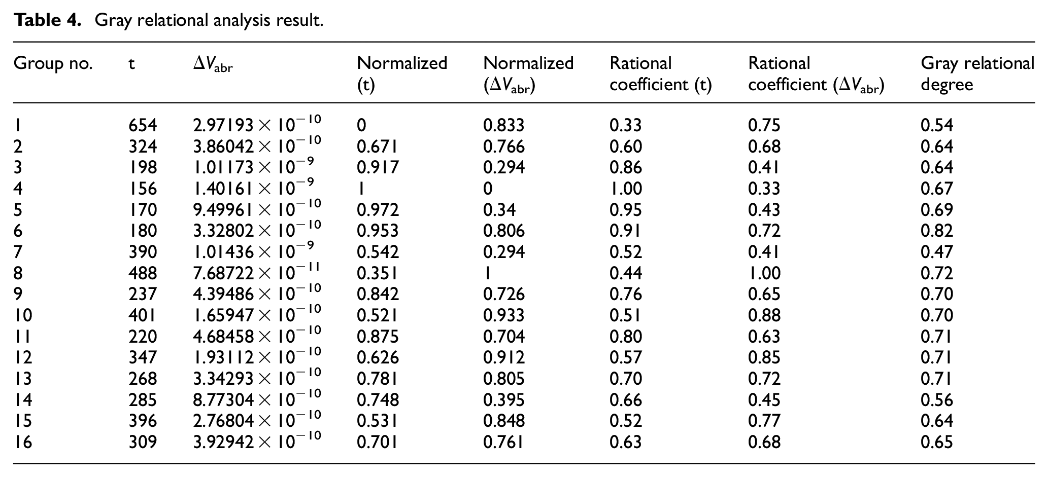
Determine the input process parameters as shown in Table 2, a total of 16 sets of data and 5 factors. They are: tool diameter, spindle speed, feed speed, axial depth of cut, and radial depth of cut. The output process parameters are the processing time (indicated by t in s) and the abrasive wear rate increment of the flank face (indicated by ΔV_abr in mm³/s), according to formula 6, the results are shown in Table 3.

It can be known by analyzing the input and output process parameters: the relational law between processing time, flank surface abrasive wear rate increment and input process parameters is inconsistent. In order to improve the processing efficiency and reduce the increase in abrasive wear rate, the gray relational method is further carried out on the basis of the orthogonal experiment.

Dimension normalization

Gray relational method is based on the data columns of factors, mathematical methods is used to study the geometric correspondence between factors and rational degree is used to measure the completion of multiple indicators.^20–24

Dimension normalization: dimension normalization is performed according to formula 7, to avoid the influence of the unit and prepare for the next step of relational calculation. Through analysis, it can be known that the smaller the increase in processing time and abrasive wear rate increment, the better. The normalized calculation uses the large characteristic formula. That is, the larger the normalized data, the more the expected value.

x = \frac{max y - y}{max y - min y}

(7)

In the formula, x represents the normalized result, y represents the output process parameter result, and the dimension normalized result is shown in Table 4.

Table 4.

Gray relational analysis result.

Group no.	t	ΔV_abr	Normalized (t)	Normalized (ΔV_abr)	Rational coefficient (t)	Rational coefficient (ΔV_abr)	Gray relational degree
1	654	2.97193 × 10⁻¹⁰	0	0.833	0.33	0.75	0.54
2	324	3.86042 × 10⁻¹⁰	0.671	0.766	0.60	0.68	0.64
3	198	1.01173 × 10⁻⁹	0.917	0.294	0.86	0.41	0.64
4	156	1.40161 × 10⁻⁹	1	0	1.00	0.33	0.67
5	170	9.49961 × 10⁻¹⁰	0.972	0.34	0.95	0.43	0.69
6	180	3.32802 × 10⁻¹⁰	0.953	0.806	0.91	0.72	0.82
7	390	1.01436 × 10⁻⁹	0.542	0.294	0.52	0.41	0.47
8	488	7.68722 × 10⁻¹¹	0.351	1	0.44	1.00	0.72
9	237	4.39486 × 10⁻¹⁰	0.842	0.726	0.76	0.65	0.70
10	401	1.65947 × 10⁻¹⁰	0.521	0.933	0.51	0.88	0.70
11	220	4.68458 × 10⁻¹⁰	0.875	0.704	0.80	0.63	0.71
12	347	1.93112 × 10⁻¹⁰	0.626	0.912	0.57	0.85	0.71
13	268	3.34293 × 10⁻¹⁰	0.781	0.805	0.70	0.72	0.71
14	285	8.77304 × 10⁻¹⁰	0.748	0.395	0.66	0.45	0.56
15	396	2.76804 × 10⁻¹⁰	0.531	0.848	0.52	0.77	0.64
16	309	3.92942 × 10⁻¹⁰	0.701	0.761	0.63	0.68	0.65

The rational coefficient

The gray relational coefficient is calculated according to formula 8, that is, the relationship between the actual output process parameters and the output process parameters in the ideal state is calculated.

ξ_{i} = \frac{min | x^{0} - x | + ζ \max | x^{0} - x |}{| x^{0} - x | + ζ max | x^{0} - x |}

(8)

In the formula: $ξ_{i}$ is the rational coefficient of the i-th actual output process parameter, total 16 sets of output process parameters. x⁰ is the ideal output process parameter, the ideal output process parameter for processing time and abrasive wear rate increment are 1. $ζ$ is the resolution coefficient, the value range is:

\frac{Δ i}{Δ max} \leq ζ \leq 2 \frac{Δ i}{Δ max}

(9)

Δi is the mean value of the difference between the ideal value and the actual value of all output process parameters:

Δ i = \frac{1}{32} | x^{0} - x |

(10)

Δmax is the maximum value of the difference between the ideal value and the actual value of the output process parameter:

Δ \max = \max | x^{0} - x |

(11)

The range of $ζ$ obtained by calculation is 0.3469 ≤ $ζ$ ≤ 0.6938, take $ζ$ = 0.5. The rational coefficient is shown in Table 4.

The gray relational degree and parameter optimization

The gray relational degree is calculated according to formula 12:

γ = \frac{1}{i} \sum_{i = 1}^{m} ξ_{i}

(12)

m is the number of actual output process parameter and m = 2. The gray relational degree is shown in Table 4.

From Table 4, it can be concluded that the gray rational degree of the sixth experiment is 0.82, which is the maximum. At this time, the input process parameter values are as follows: the tool diameter is 8 mm, the spindle speed is 2000 rpm, the feed speed is 460 mm/min, the axial depth of cut is 12 mm, and the radial depth of cut is 2 mm. However, the processing time is 180 s and the abrasive wear rate increment is 3.32802 × 10⁻¹⁰ mm³/s, neither data is the smallest. It shows that current parameters may be further optimized. It is necessary to further analyze the average value and range of the gray relational degree of input process parameters to obtain better parameters. The average and range analysis results of the gray relational of input process parameters are shown in Table 5.

Table 5.

Average and range analysis of gray relational degree of input process parameters.

Level	Ф	Average	s	Average	f	Average	a _p	Average	a _e	Average
1	6	0.621	1800	0.661	460	0.681	6	0.568	1	0.650
2	8	0.673	2000	0.677	480	0.671	8	0.696	1.5	0.616
3	10	0.706	2200	0.616	500	0.654	10	0.670	2	0.718
4	12	0.641	2400	0.688	520	0.635	12	0.707	2.5	0.657
Range		0.085		0.08		0.046		0.139		0.102

Draw a graph of the relationship between input process parameters and the average gray relational degree, as shown in Figure 4 (the ordinate represents the average gray relational degree of input parameters). When the average value of a certain level of gray relational in the figure reaches the maximum, the input process parameter of this level is the optimal value. By the relationship curve is analyzed, we can see that the optimal parameters are: the tool diameter is 10 mm, the spindle speed is 2400 rpm, the feed speed is 460 mm/min, the axial depth of cut is 12 mm, and the radial depth of cut is 2 mm.

Figure 4.

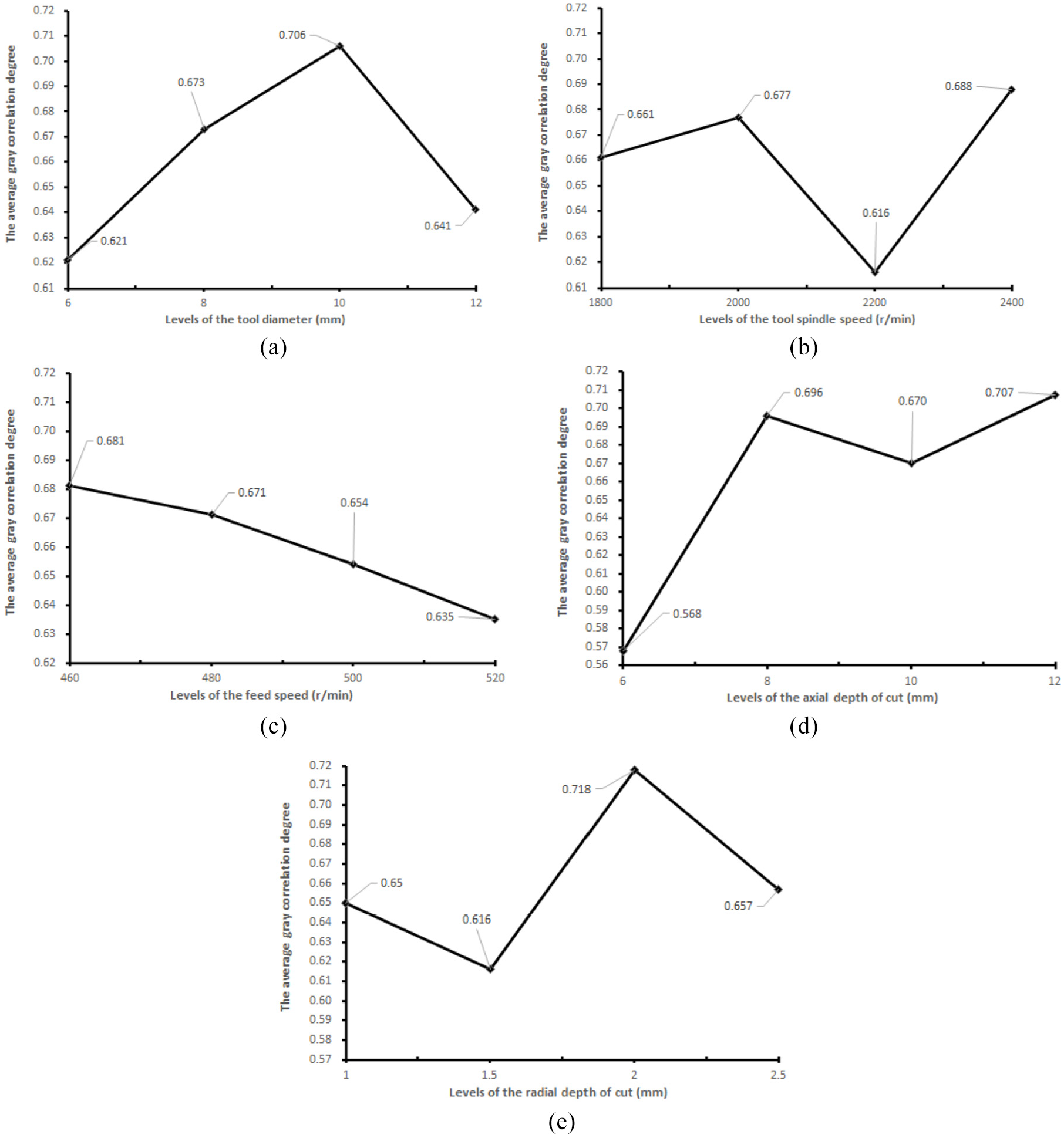
Graph of the relation between the input process parameters and the mean value of gray relational degree: (a) tool diameter, (b) spindle speed, (c) feed speed, (d) axial depth of cut, and (e) radial depth of cut.

The optimal parameters obtained by the gray relational method with the optimal parameters of the orthogonal experiment are compared. As shown in Table 6:

Table 6.

Comparison of experiment results.

	Ф	s	f	a _p	a _e	$t$	ΔV_abr	Gray relational degree
Orthogonal test optimal combination	8	2000	460	12	2	180	3.32802 × 10⁻¹⁰	0.82
Gray relational analysis optimal combination	10	2400	460	12	2	179	2.90379 × 10⁻¹⁰	0.84

Incremental prediction model

Back Propagation (BP) neural network is a multi-layer feed forward network trained by error back propagation algorithm.^25–27 It is the most widely used neural network technology in predictive models. In this paper, the BP neural network technology is used to build the flank face abrasive wear rate incremental prediction model.

The application of BP neural network technology in the prediction model of abrasive wear rate increment is as follows: the tool diameter, spindle speed, feed rate, axial depth of cut, and radial depth of cut in the orthogonal experiment are taken as the input layer data. The flank surface abrasive wear rate increment and processing time are used as output layer data. The relationship between the input layer data and the output layer data is established by training the neural network and it can achieve the required training accuracy.

The basic network structure

The BP neural network is composed of an input layer, a hidden layer, and an output layer. Three layers are fully connected through the weight matrix and bias. Experiments show that a three-layer BP neural network can complete a mapping from any n-dimensional input layer to m-dimensional output layer.^28–30 This paper adopts a three-layer BP neural network model, as shown in Figure 5, w_ih and w_hj are the weights between layers, and q is the bias.

Figure 5.

Neural network structure diagram.

Determination of basic parameters

Trial and error method is used to determine the number of hidden layer neurons, as shown in formula 13:

L = \sqrt{m + n} + a

(13)

m is the number of neurons in the input layer, n is the number of neurons in the output layer. a is a constant, 0 ≤ a ≤ 10. L is the number of neurons in the hidden layer. It can be concluded that the range of the number of neurons in the hidden layer is: 2 ≤ L ≤ 12. According to the principles of ensuring the prediction accuracy and the stability of the neural network, the number of neurons is finally determined to be 9. The choice of learning rate is based on the principles of avoiding neural network fluctuations and fast convergence, the learning rate is 0.002. The activation function is the sigmoid function as shown in formula 14:

y = \frac{1}{1 + e^{- x}}

(14)

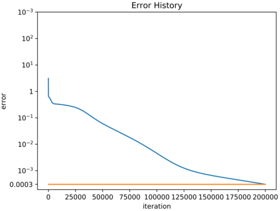
The maximum number of iterations is 200,000 and the training target error is 0.0003. To prevent over fitting, add noise to the output sample, the noise intensity is 0.03. The input layer data are normalized by the formula 15:

x^{*} = 2 \frac{x - x_{min}}{x_{max} - x_{min}} - 1

(15)

x _max and x_min represent the maximum and minimum values in each type of data, the normalized data range are −1 ≤ x* ≤ 1. Initialize the weight and offset, the range is 0–0.5, the cost function is shown in formula 16:

Δ = \sum_{i = 1}^{16} {(y_{i}^{'} - y_{i})}^{2}

(16)

$y_{i}^{'}$ represents the actual output value and $y_{i}$ represents the neural network output value, the iteration ends when Δ < 0.0001.

Key program segments and training results

#Dynamic adjustment of each step based on the principle of negative gradient descent of the cost function

del2=error

del1=np.dot(w2.transpose(),del2)*hidout*(1-hidout)

dw2 = np.dot(del2,hidout.transpose())

db2 = np.dot(del2,np.ones((samnum,1)))

dw1=np.dot(del1,sampleinnorm.transpose())

db1 = np.dot(del1,np.ones((samnum,1)))

#Modify the weights and thresholds between the output layer and the hidden layer

w2 = w2 +lerate*dw2

b2 =b2 + lerate*db2

#Modify the weight and threshold between the input layer and the hidden layer

w1 = w1lerate*dw1

b1 =b1 + lerate*db1

See Supplemental Files for various groups.

The network error performance training curve is shown in Figure 6, the iteration ends when the number of iterations reaches 200,000 times, error value is 0.0003. The fitting result of the training prediction value and the actual value are shown in Figure 7.

Figure 6.

BP network error performance training curve.

Figure 7.

The predicted training values were fitted with the actual values.

Conclusions

Through gray relational analysis, the following conclusions can be made:

From the relational value, it can be seen that the maximum gray relational value of the radial cutting depth is 0.139. It shows that the axial depth of the cut has the most significant comprehensive influence on the machining time and the abrasive wear rate increment of the flank face. The radial depth of cut is the second important factor to affect the time and wear, followed by the tool diameter, spindle speed, and feed rate.

In the case of non-increasing processing time, tool wear can be slowed by increasing the following items: the tool diameter and the spindle speed. Under the conditions that the feed speed, axial depth of cut, and radial depth of cut are given, the work piece’s contour has no restriction on the tool diameter, these two items’ deduction mainly affects the tool wear.

In the case of non-increasing processing time, the following conclusions can be made by analyzing the relationship between the input process parameters and the abrasive wear rate increment of the flank face. The influence of the input process parameters on the abrasive wear rate increment can be expressed by the following inequality: a_e > Ф > s > a_p > f.

In the case of non-increasing processing time, aiming to reduce the tool wear rate, the basic principle of parameter selection for CNC milling is the five factors should be small. However, in high-speed milling, there is a spindle speed limit for the milling cutter. If the spindle speed exceeds this limit, the wear decreases. How to determine the limit of spindle speed should be a new research topic.

A prediction model for the abrasive wear rate increment of the flank face is established, and the prediction value is compared with the actual value. It is found that the BP neural network can predict the abrasive wear rate increment of the flank face and has good accuracy and stability. From the perspective of tool wear rate increment, it provides practical methods and new ideas for monitoring tool wear status.

Supplemental Material

sj-pdf-1-ade-10.1177_16878140211039972 – Supplemental material for Optimization of milling process parameters and prediction of abrasive wear rate increment based on cutting force experiment

Supplemental material, sj-pdf-1-ade-10.1177_16878140211039972 for Optimization of milling process parameters and prediction of abrasive wear rate increment based on cutting force experiment by Fei Li and Jun Liu in Advances in Mechanical Engineering

Footnotes

Handling Editor: James Baldwin

Declaration of conflicting interests

The author(s) declared no potential conflicts of interest with respect to the research, authorship, and/or publication of this article.

Funding

The author(s) disclosed receipt of the following financial support for the research, authorship, and/or publication of this article: This work was supported by State key R & D plan of the Ministry of science and technology of the People’s Republic of China (Grant No. 2018YFB1703105).

ORCID iD

Fei Li

Supplemental material

Supplemental material for this article is available online.

References

Tian

Zhang

. Modeling and multi-objective optimization of cutting parameters in the high-speed milling using RSM and improved TLBO algorithm. Int J Adv Manuf Technol 2020; 111: 2323–2335.

Shi

Zhang

Ren

. Optimization of process parameters for surface roughness and microhardness in dry milling of magnesium alloy using Taguchi with grey relational analysis. Int J Adv Manuf Technol 2015; 81: 645–651.

Chen

Xie

, et al. Optimization of process parameters in the high-speed milling of titanium alloy TB17 for surface integrity by the Taguchi-Grey relational analysis method. Adv Mech Eng 2016; 8: 168781401667144

Tong

Liu

. Support vector regression and genetic-algorithm-based multi-objective optimization of mesoscopic geometric characteristic parameters of ball-end milling tool. Proc IMechE, Part B: J Eng Manuf 2020; 234: 1333–1345.

Shang

Yan

, et al. Reliability design optimization of milling process parameters based on approximate model. China Mech Eng 2019; 30: 106–111.

Sarıkaya

Yılmaz

Dilipak

, et al. Modeling and multi-response optimization of milling characteristics based on Taguchi and gray relational analysis. Proc IMechE, Part B: J Engineering Manufacture 2016; 230: 1049–1065.

Zhang

Zou

, et al. Research on tool wear prediction based on Archard agglomeration scavenging theory. Adv Mech Eng 2017; 9: 168781401772408.

Chen

. An artificial-neural-networks-based in-process tool wear prediction system in milling operations. Int J Adv Manuf Technol 2005; 25: 427–434.

Wen

Chaoyong

Leilei

, et al. Prediction model of milling cutter wear status based on deep learning. China Mech Eng 2020; 31: 2071–2078.

10.

Ding

Bai

Liu

, et al. A novel method for tool wear prediction in titanium milling by simulink feedback method. J Mech Eng 2019; 55: 224–232.

11.

Cao

Sun

Zhang

, et al. In process tool condition monitoring based on convolution neural network. Comput Integr Manuf Syst 2020; 26: 74–80.

12.

Cus

Zuperl

. Real time cutting tool condition monitoring in milling. J Mech Eng 2011; 57: 142–150.

13.

Wang

. CHMM for tool condition monitoring and remaining useful life prediction. Int J Adv Manuf Technol 2012; 59: 463–471.

14.

Shen

Zhang

Yao

, et al. Formation mechanism of surface metamorphic layer and influence rule on milling TC17 titanium alloy. Int J Adv Manuf Technol 2021; 112: 2259–2276.

15.

Shen

Zhang

Tan

. Effects of cutter path orientations on milling force, temperature, and surface integrity when ball end milling of TC17 alloy. Proc IMechE, Part B: J Engineering Manufacture 2021; 235: 1212–1224.

16.

Zhu

Sun

, et al. Investigation on the influence of tool wear upon chip morphology in end milling titanium alloy Ti6Al4V. Int J Adv Manuf Technol 2016; 83: 1477–1485.

17.

Bermingham

Sim

Kent

, et al. Tool life and wear mechanisms in laser assisted milling Ti–6Al–4V. Wear 2015; 322-323: 151–163.

18.

Qin

, et al. Tool wear and hole quality investigation in dry helical milling of Ti-6Al-4V alloy. Int J Adv Manuf Technol 2014; 71: 1511–1523.

19.

Huang

Liang

. Modeling of CBN tool flank wear progression in finish hard turning. J Manuf Sci Eng 2004; 126: 98–106.

20.

Laxman

Raj

DKG

. Optimization of EDM process parameters on titanium super alloys based on the grey relational analysis. Int J Eng Res 2014; 3: 344–348.

21.

Chiu

Gan

Tseng

, et al. Multi-objective optimization of process parameters in an area-forming rapid prototyping system using the Taguchi method and a grey relational analysis. Proc IMechE, Part B: J Engineering Manufacture 2017; 231: 2211–2222.

22.

Varun

Venkaiah

. Grey relational analysis coupled with firefly algorithm for multi-objective optimization of wire electric discharge machining. Proc IMechE, Part B: J Engineering Manufacture 2015; 229: 1385–1394.

23.

Shi

Zhang

Ren

, et al. Multiobjective optimization of surface integrity in milling TB6 alloy based on Taguchi-Grey relational analysis. Adv Mech Eng 2014; 6: 280313–280317.

24.

Ayaz

Khaki

Arab

NBM

. Improvement of grain size and dome height of microalloyed steels using Taguchi method based on grey relational grade in controlled rolling. J Iron Steel Res Int 2013; 20: 115–123.

25.

Zou

Liao

Zeng

, et al. An improved BP neural network based on evaluating and forecasting model of water quality in Second Songhua River of China. Chin J Geochem 2006; 25: 167–167.

26.

Liu

, et al. Research on al-gorithmic power consumption BP net-work model of embed-ded software. J Univ Electron Sci Technol China 2011; 40: 921–926.

27.

Aylı

. Modeling of mixed convection in an enclosure using multiple regression, artificial neural network, and adaptive neuro-fuzzy interface system models. Proc IMechE, Part C: J Mechanical Engineering Science 2020; 234: 3078–3093.

28.

Bing

Pengbo

Yan

, et al. Research on processor energy saving strategy based on BP neural net-work. Adv Eng Sci 2018; 50: 107–112.

29.

Zheng

Wang

Sun

, et al. Aero-engine direct thrust control with nonlinear model predictive control based on linearized deep neural network predictor. Proc IMechE, Part I: J Syst Control Eng 2020; 234: 330–337.

30.

Wang

Guo

, et al. Quality prediction and control of cable harness wiring using extension theory and a backpropagation neural network. Adv Mech Eng 2020; 12: 168781402092310.

Supplementary Material

Please find the following supplemental material available below.

For Open Access articles published under a Creative Commons License, all supplemental material carries the same license as the article it is associated with.

For non-Open Access articles published, all supplemental material carries a non-exclusive license, and permission requests for re-use of supplemental material or any part of supplemental material shall be sent directly to the copyright owner as specified in the copyright notice associated with the article.

0.00 MB

1.52 MB