Probabilistic analysis of crack growth in railway axles using a Gaussian process

Abstract

To reduce maintenance costs, it is important to carry out probabilistic analyses on railway vehicle components. In this work, a data-driven approach based on a Gaussian process for regression is developed to determine the probability of axle failure caused by crack growth in railway axles. For complicated failure modes, it is difficult or even impossible to build a reliable analytical or simulation model before using an analytical approach. The main purpose of this work is to develop an algorithm to infer the distribution of crack growth from limited measured data without having to build an underlying model. The results of the case study show that the determined timing for the first inspection and the probability of failure coincide with the known results derived by analytically based approaches. The problems associated with modelling and calibration can be overcome by a data-driven approach. The developed Gaussian process model can serve as a complementary instrument to validate other analytically based approaches or numerical analyses. The model can also be applied to the probabilistic analyses of other railway components.

Introduction

Preventive maintenance is a prevailing principle in the railway industry. Consequently, maintenance activities are scheduled according to the number of travelled kilometres or the operating time of a railway component. An optimal maintenance plan is desired to reduce maintenance costs. The engineering discipline of reliability, availability, maintainability and safety (RAMS) should be fully considered; specifically, reliability analysis is carried out to ensure that the resulting risk of a maintenance plan is below a tolerable level. Since many stochastic aspects are involved in railway operations and maintenance, probabilistic analysis is applied to assess reliability.

The service life of railway axles can be more than 30 years with a high number of loading cycles. During the whole life cycle, several inspection and maintenance activities should be planned. An example of defining inspection intervals is illustrated in Figure 1. The probability of failure (PoF) is calculated during the service life. Before the PoF reaches the tolerable PoF, an inspection should be planned so that the PoF can be reduced again. At each inspection, an axle with a crack size that exceeds the detectable size will be identified. The axle will be repaired or put out of service. However, there are still many very small, undetectable cracks remaining on the axles. In the beginning, the growth rate of these small cracks is very slow. After a certain period of service, the accumulated loading effects will lead to a rapid increase in crack size. Therefore, the inspection interval will shorten over time. Traditional maintenance programmes are set in a fixed inspection interval. For example, an ultrasonic inspection should be carried out for a China Railway Rolling Corporation (CRRC) China Railway High-Speed (CRH)-2 high-speed train at each 90,000 km interval (approximately 3.5 × 10⁷ rotation cycles). High maintenance costs will result from following a maintenance plan with overly short inspection intervals. However, if the inspection interval is too long, a crack may reach an intolerable depth before the next inspection, possibly leading to derailment. In this context, the objective of a probabilistic analysis is to find the maximum inspection interval that ensures that the PoF is under an acceptable level.

Figure 1.

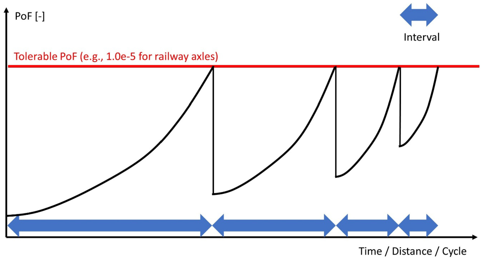
Definition of maintenance intervals based on the PoF.

In the study by Zerbst et al., ¹ the mechanism of crack initiation in railway axles and the methods of determining a safe service life and damage tolerance are reviewed. Meanwhile, several research projects are being carried out in Europe, including EisenBahn FahrWerke (EBFW), ² Bundesministerium für Bildung und Forschung (BMBF; German abbreviation for federal ministry of education and research) Project 19 P 0061 A–F 6, ³ and wheelset integrated design and effective maintenance (WIDEM). ⁴ In recent years, an investigation of crack growth and the optimisation of a maintenance plan for the Chinese railway high-speed (CRH) system has received great attention as well. This work focuses on developing a probabilistic analysis of the crack growth in railway axles and uses railway axles for CRH trains as a case study.

As the distance and number of cycles increase over time, the inspection intervals will be shortened during the whole service life (see Figure 1). Instead of determining all the inspection intervals, this work calculates only the first inspection interval to evaluate the proposed method. The development of a maintenance plan during the whole service life will be investigated in future research.

In this article, the approaches for the probabilistic analysis of crack growth will be reviewed in section ‘Analytical, numerical and data-driven approaches for the probabilistic analysis of crack growth’. The constraints of analytically based approaches and numerical analyses are discussed. In section ‘Probabilistic analysis using a GP’, a data-driven approach based on a Gaussian process (GP) is proposed. The case study and the results are presented in section ‘Case study: regression with probabilistic layers’. The findings, the limitations of this work, and future directions are discussed in section ‘Conclusion and discussions’.

Analytical, numerical and data-driven approaches for the probabilistic analysis of crack growth

Martinez et al. ⁵ summarised the approaches for analysing the crack growth in railway axles, including the analytically based approach, the numerical analysis and the data-driven approach. These approaches can also be applied to probabilistic analysis. The main difference among these approaches is the mechanism for modelling the crack growth.

In the analytically based approach, the crack growth and propagation are modelled by using mathematical equations. In this work, Paris’ law ⁶ is applied to describe a power law relationship between the rate of crack growth and changes in the stress intensity factor (SIF). The SIF is derived from the stress, the crack depth and the geometry factor, depending on the loading and cracked body configuration. Paris’ law and the calculation of the SIF are shown in equations (1)–(3)

$$K=\delta Y\sqrt{\pi a}$$

(1)

$$\mathrm{\Delta }K=K_{\max }-K_{\min }$$

(2)

$$\frac{\mathrm{da}}{\mathrm{dN}}=C\mathrm{\Delta }{K}^m$$

(3)

By integrating the differential equation (3), the crack growth will be solved for a certain number of cycles. In railway operations, the number of cycles can also be mapped to other dimensions, such as time or distance. In this article, a simplified implementation of Paris’ law based on time is applied (see section ‘Data preparation and calculation of the PoF based on the FORM/SORM’) to generate sampled data and to verify the developed algorithm.

With the analytical model, the reliability of the system and the PoF can be estimated. In probabilistic analysis, multiple random variables and their joint distribution should be considered. In the study by Zhu et al., ⁷ the uncertainty quantification (UQ) is applied with multiplicative and additive methods, in order to identify and quantify the contribution of uncertainty from multiple types. Combined with classical statistics and data-driven approaches, the probabilistic model is updated through a Bayesian inference with experiment results. The first-order reliability method (FORM) and the second-order reliability method (SORM) have been widely used as an analytically based approach in recent decades. ⁸ Given the analytical model, a limit state function can be defined to describe the boundary between the safe and failure states. By transforming the multiple correlated variables from physical space to a standardised uncorrelated space, the PoF can be calculated through a reliability index. Currently, the FORM and SORM have been implemented as standard features in many reliability analysis software programmes, for example, DAKOTA, OpenTURNS, SYSREL and PyRe. In this work, OpenTURNS is used to calculate the PoF based on an analytically based approach (see section ‘Data preparation and calculation of the PoF based on the FORM/SORM’).

The difficulty in using an analytically based approach increases with complicated crack geometries and different failure modes. Sometimes, it is even impossible to solve the partial differential equations in an analytical model. Supported by finite element method (FEM), numerical analysis is used to solve dynamic equations. The required inputs for numerical analysis are the component’s geometry, initial cracks, properties of the materials, loading conditions, and other boundary and support conditions. During a simulation, the propagation of a crack and the other properties (e.g. stresses and SIF) can be obtained for further analysis.

Several commercial software programmes, for example, Zencrack and NASGRO, are available for fracture and fatigue analysis. These software programmes can be integrated with finite element software and software for reliability and uncertainty analysis. Software application and development are also very active in railway sectors. For example, the NASGRO model ⁹ is used in the WIDEM project; ¹⁰ the software INARA integrated with DAKOTA is developed for the probabilistic analysis in the EBFW-3 project, ¹¹ and the programme ERWIN is developed to determine inspection intervals. ³

Most research of crack growth and propagation on railway axles are concerned at individual cracks. It is difficult to investigate the characteristics of crack coalescence with an analytically based approach. In the study by Zhu et al., ¹² a probabilistic procedure for multiple surface fracture simulation is established. The behaviour of crack formation and propagation can be simulated with randomly generated parameters, including the positions and initial size of cracks, properties of the materials and fatigue crack growth rate. The failure modes, the probabilistic model of multiple surface cracking are further studied in Zhu et al. ¹³ The remaining usage lives from initial cracks to critical cracks can be estimated from the probabilistic model.

The authors use the numerical approach to simulate crack growth for railway axles. The finite element model of a non-defective railway axle is built with the FE software Abaqus. The tool Zencrack for fracture mechanics simulations is used to simulate the progress of crack growth for a randomly generated initial crack. The progress of crack growth, including the size and the depth of the crack, stress and strain values, SIFs, J-integral values, Ct-integral values and T-stress values, can be read and evaluated from the simulation results (see Figure 2). Since the numerical analysis for the prediction of crack growth is very time-consuming, a method for predicting crack growth in railway axles with artificial neural network (ANN) is developed. The initial crack depth and crack growth can be predicted through the trained ANN, which coincides with the simulated FE analysis results.

Figure 2.

FEM analysis of crack growth in a railway axle.

Both the analytically based approach and numerical analysis require an accurate model to represent crack growth. The model should be calibrated by comparing the results from the model and the measured value from reality. The available measured data provide an option for the data-driven approach. With the data-driven approach, the measured data can be used directly to infer the behaviour of the system without having to build an analytical or simulation model. Due to the rapid development of machine learning and large data in recent years, the data-driven approach has been successfully applied in many applications. In the study by Cunha et al., ¹⁴ the methods for applying the backmapping approach, the adaptive Gaussian method and the unscented filter method are compared with analytically based approaches and Monte Carlo methods. The results show that these data-driven approaches can achieve higher accuracy than the FORM and lead to a considerably smaller computation time than simulation-based approaches.

Essentially, there is a very strong assumption behind the analytical and numerical approaches: the existence and the mechanism of crack growth should be known before using probability analysis. If the eventuality of crack growth is not based only on assumptions, the problem can be overcome through a data-driven approach. Since prior knowledge of the system is no longer conceived as fixed, the algorithm is capable of learning and dramatically evolving. If the amount of data is limited, the data-driven approach can still draw conclusions from the available data. With increasing amounts of collected data, the results of the analysis can be continuously improved. Indeed, this is also the key idea behind Bayesian inference, which has been successfully used to solve stochastic problems, including those addressed by probabilistic analysis and uncertainty analysis.

Inspired by the idea that increasingly more data can improve analysis, a data-driven approach with a GP is proposed in this work. With the model, the workflow for calculating the PoF can be divided into a training process and a prediction process. In section ‘Prediction of the PoF with a GP model’, an introduction to the regression model using a GP to predict the PoF is given. The procedure to train a GP model is described in section ‘Training a GP model’.

Probabilistic analysis using a GP

Prediction of the PoF with a GP model

In applying probabilistic analysis to crack growth, the available information is a set of measured data which consists of the measurement time $\mathit{t}=\{t_i|i=1,2,\dots ,n\}$ and the crack depth $\mathit{a}=\{a_i|i=1,2,\dots ,n\}$ . With the given information, the objective of probabilistic analysis is to determine the distribution $p$ of the crack depth at any time point. Hence, the PoF can be determined from $p$ . However, it is difficult to calculate the underlying distribution $p$ directly: either a closed mathematical form is not available, or the computational complexity is very high. ¹⁵ Therefore, a regression model can be applied to learn from the measured data and predict the distribution of the crack depth.

With the regression model, distribution $q$ is used to approximate the true distribution $p$ . This approximated distribution $q$ should be easily built with a known form. The GP model is a powerful tool that has been successfully applied in machine learning for regression and classification. ¹⁶ In this work, the tasks of crack growth analysis in the GP model involve training the model and predicting the approximated distribution $q$ at any given time. The inputs of the GP model are the measured crack depth and measurement time, without having to model the internal variable including the load spectra and SIFs. The output of the prediction model is the distribution of the crack depth for a given time point $\mathit{t}\prime$ .

A GP model is defined by a mean function $m(t)$ and a covariance function $k(t,t\prime )$ with the parameter $\theta$ . In section ‘Training a GP model’, the definition of these functions and the process to fit the parameters will be explained in detail. A fitted GP model with trained parameters for mean and covariance functions generates random data such that any finite subset of the generated data follows a multivariate Gaussian distribution. The model creates the possibility of producing the distribution of the crack depth $\mathit{a}\prime$ for any new time points $\mathit{t}\prime$ with the given measured data $\mathit{a}$ and $\mathit{t}$ as

$$\left[\begin{array}{c}\mathit{a}\hfill \\ \multicolumn{1}{c}{\mathit{a}\prime }\end{array}\right]~\mathcal{N}(\left[\begin{array}{c}\mu \hfill \\ \multicolumn{1}{c}{\mu \prime }\end{array}\right],\left[\begin{array}{c}{\mathrm{\Sigma }}_{\mathrm{tt}},{\mathrm{\Sigma }}_{\mathrm{tt}\prime }\hfill \\ \multicolumn{1}{c}{{\mathrm{\Sigma }}_{t\prime t},{\mathrm{\Sigma }}_{t\prime t\prime }}\end{array}\right])$$

(4)

with

$$\mu =m\left(\mathit{t}\right),\mu \prime =m(\mathit{t}\prime )$$

$${\mathrm{\Sigma }}_{\mathrm{tt}}=k(\mathit{t},\mathit{t}),{\mathrm{\Sigma }}_{t\prime t\prime }=k(\mathit{t}\prime ,t\prime )$$

$${\mathrm{\Sigma }}_{\mathrm{tt}\prime }=k(\mathit{t},\mathit{t}\prime ),{\mathrm{\Sigma }}_{t\prime t}=k(\mathit{t}\prime ,\mathit{t})$$

As defined in equation (4), the time points and the crack depth at each time point are the correlated variables in a GP. The vector of the mean and the covariance matrix in equation (4) can be calculated from the mean function and the kernel function, respectively. In addition, the noise in the measured data will also be considered; the noise will be added as noise variance ${\sigma }_{\epsilon }^2$ to the covariance ${\mathrm{\Sigma }}_{\mathrm{tt}}$ and ${\mathrm{\Sigma }}_{t\prime t\prime }$ . The value of the noise variance will also be trained in the GP model.

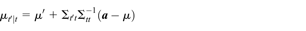
To predict the distribution of the crack depth $\mathit{a}\prime$ for new time points $\mathit{t}\prime$ , the approximated posterior distribution $q(\mathit{a}\prime |\mathit{a},t,t\prime )$ can be calculated as

$$q(\mathit{a}\prime |\mathit{a},t,t\prime )~\mathcal{N}({\mu }_{t\prime |t},{\mathrm{\Sigma }}_{t\prime |t})$$

(5)

with

$${\mu }_{t\prime |t}=\mu \prime +{\mathrm{\Sigma }}_{t\prime t}{\mathrm{\Sigma }}_{\mathrm{tt}}^{-1}(\mathit{a}-\mu )$$

$${\mathrm{\Sigma }}_{t\prime |t}={\mathrm{\Sigma }}_{t\prime t\prime }-{\mathrm{\Sigma }}_{t\prime t}{\mathrm{\Sigma }}_{\mathrm{tt}}^{-1}{\mathrm{\Sigma }}_{\mathrm{tt}\prime }$$

From the posterior distribution $q(\mathit{a}\prime |a,t,t\prime )$ , the mean ${\mu }_{t\prime |t}$ and the standard deviation ${\mathrm{\Sigma }}_{t\prime |t}$ at $\mathit{t}\prime$ will be derived. A Gaussian distribution with the mean ${\mu }_{t\prime |t}$ and the standard deviation ${\mathrm{\Sigma }}_{t\prime |t}$ will be constructed. The PoF is then calculated from its cumulative distribution function (CDF) for the given critical depth. Hence, the distribution of the crack depth and the PoF at a certain time point can be predicted by the GP regression model.

Training a GP model

As described in section ‘Prediction of the PoF with a GP model’, a GP is defined by a mean function and a covariance function with the parameter $\theta$ . The task of training a GP model involves identifying suitable parameters for these functions. The mean function can be set as the mean value of the measured data $\mathit{a}$ . It is also very common to set the mean function to 0 since the covariance function is able to capture and model the characteristics of the GP model.

For a probabilistic analysis of crack growth, the covariance is defined by a kernel function $k(t,t\prime )$ between two time points $t$ and $t\prime$ . The kernel function describes the correlation between any two points. The key principle of setting a kernel function is that if $t$ and $t\prime$ are very close, the expected output distribution of the function should also be similar. The commonly used kernel functions for GPs include an exponential quadratic function, a rational quadratic function, a local periodic function, a linear function and combing kernels. In the study by Rasmussen and Williams ¹⁶ and Murphy, ¹⁷ the covariance and design of a kernel function are explained in detail. In this work, the exponential quadratic kernel is used

$$k(t,t\prime )={\sigma }^2·e^{-\frac{{(t-t\prime )}^2}{2{\ell }^2}}$$

(6)

In equation (6), the value $t-t\prime$ represents the difference between two points. If the value is close to zero, this condition will lead to a maximum value of the kernel as ${\sigma }^2$ , thereby indicating that the two points are highly correlated. If the value $t-t\prime$ is very large, the correlation of the two points can be neglected with $k(t,t\prime )\approx 0$ .

The exponential quadratic kernel function is stationary; this stationary state only depends on the relative position of two time points $t$ and $t\prime$ . With the increase in time, the mean value and the variance of the crack depth will also increase. To represent the dependency of the absolute position, an additional scale factor for the variance is introduced to multiply the mean value of the crack depth.

The parameters $\sigma$ and $\ell$ , the scale factor of the variance and the noise variance ${\sigma }_{\epsilon }$ (see section ‘Prediction of the PoF with a GP model’) will be learned during the training process. The general term $\theta$ is used to refer to all the trainable parameters. During a training process, the given measured data will be batched as $\tilde{\mathit{t}}$ and $\tilde{\mathit{a}}$ in many iterations. To derive the approximated distribution $q$ for the batched data $\tilde{\mathit{t}}$ and $\tilde{\mathit{a}}$ , the parameters $\theta$ should be trained to maximise the marginal likelihood $q(\tilde{\mathit{a}}|\tilde{\mathit{t}},\theta )$

$${\theta }^{*}=\underset{\theta }{\mathrm{argmax}}q(\tilde{\mathit{a}}|\tilde{\mathit{t}},\theta )=\underset{\theta }{\mathrm{argmin}[}-\log \left(q(\tilde{\mathit{a}}|\tilde{\mathit{t}},\theta )\right)]$$

(7)

$$\begin{array}{c}\multicolumn{1}{c}{\log \left(q(\tilde{\mathit{a}}|\tilde{\mathit{t}},\theta )\right)=-\frac{1}{2}{(\tilde{\mathit{a}}-{\mu }_{\theta })}^{\top }{{\mathrm{\Sigma }}_{\theta }}^{-1}(\tilde{\mathit{a}}-{\mu }_{\theta })}\\ \multicolumn{1}{c}{-\frac{1}{2}\log \left|{\mathrm{\Sigma }}_{\theta }\right|-\frac{d}{2}\log 2\pi }\end{array}$$

(8)

In equation (7), the optimal parameters ${\theta }^{*}$ are derived by minimising the negative log-likelihood loss. This minimisation is equivalent to maximising the marginal likelihood since the log function is a monotone transformation. Minimising the negative log-likelihood enables a product calculation to be converted into a summation calculation. The potential for underflow can also be avoided. The negative log-likelihood is calculated in equation (8); the negative log-likelihood can be minimised through a gradient-based approach.

Many software packages implement a GP model for training and regression. In section ‘Case study: regression with probabilistic layers’, a case study of the regression of the crack growth process and a comparison of the GP model with the analytical approach will be presented.

Case study: regression with probabilistic layers

Data preparation and calculation of the PoF based on the FORM/SORM

Before starting the inference by the GP model, the data for training and validation should be prepared. Theoretically, the ‘true’ value of the PoF and the distribution of the crack depth are unknowable. To test and validate the results obtained with the GP model, a simplified analytical model is built. With the analytical model, the PoF can be calculated in advance by the FORM and SORM (see section ‘Analytical, numerical and data-driven approaches for the probabilistic analysis of crack growth’). Then, a set of data for the crack depth at different time points can be randomly generated from the analytical model. These data will be used as if they were measured in reality. In this section, the term ‘measured data’ refers to the data generated from the analytical model. The PoF estimated from the GP model will be compared with the analytical results, which are calculated with the FORM and SORM.

The log-log plot of the real crack growth rate is illustrated in Figure 3(a). Some algorithms, for example, the NASGRO equation, ⁸ are used to model the relation between the crack growth rate and the SIF range. As described in section ‘Prediction of the PoF with a GP model’, the inputs of the GP model are the measured crack depth and measurement time, and it is not required to know the information about the SIF range. To compare the results between the analytical approach and data-driven approach, reliability analysis with the FORM and SORM should be carried out with the same input information. Therefore, a closed-form solution for the crack depth depending on time is required. However, it is not possible to have such a closed mathematical formula for realistic crack growth. Hence, the crack growth rate is calculated through a simplified model. For testing and verification, Paris’ law is rewritten in a simplified way, as shown in equation (9). The solution is presented in equation (10), which is the solved form of the differential equation given in equation (9). The simplified linear function on the log–log plot is shown in Figure 3(b). The intension of this simplified model is not to calculate the real crack growth rate. Instead, it is used to provide the FORM and SORM in a closed form for reliability analysis. Meanwhile, the GP model can estimate the PoF with the data generated by the same model

$$\frac{\mathrm{da}}{\mathrm{dt}}=C·{\left(\rho \sqrt{a}\right)}^m$$

(9)

$$a={[C·\frac{(2-m)}{2}.{\rho }^m·t+a_0^{(2-m)/2}]}^{2/(2-m)}$$

(10)

Figure 3.

Illustration of the simplified closed-form solution in a log–log plot: (a) real crack growth rate and (b) simplified crack growth rate.

The critical depth of the crack is defined as $a_{\mathrm{critical}}=0.05\mathrm{m}$ . Random variables will be introduced to imitate the stochastic behaviour of crack growth. The parameters $\rho$ , $C$ and $a_0$ are random values, following a normal distribution with the given mean and standard deviation. According to British Standards Institution ¹⁸ and Beretta and Carboni, ¹⁹ the parameter $m$ is deterministic in most reliability analyses. The value of $m$ and the mean value of $C$ are taken from the material of carbon steel S38C, which is used for the railway axles of a type of CRH train produced by CRRC Qingdao Sifang Co., Ltd. Since the standard deviation of $C$ is not available, it is assumed to be 10% of the mean value according to the value provided in WIDEM. ⁴

The greatest challenge is to determine the distribution of the stress and geometry factor in the simplified model. In a fatigue crack growth model, the stress will be either modelled by the load spectra or from a known distribution of stress amplitudes. However, the real load spectra and stress distribution cannot be directly used in the simplified model. In region I shown in Figure 3(a), the crack growth rate increases very slowly with a small $\mathrm{\Delta }K$ near the threshold. The crack growth will be too fast if the simplified linear relationship in the log–log plot is applied to region I. The SORM and FORM cannot deal with a complicated piecewise function for the crack growth rate. In addition, the value $Y$ is highly dependent on the geometry of the crack. The differential equation is difficult to solve with a purely analytical approach. Usually, numerical analysis should be applied. For this reason, a simplified parameter $\rho$ combined with the stress and geometry factor is introduced. The distribution of $\rho$ is chosen to generate a set of ‘fictive’ PoFs through the FORM and SORM, which fit the empirical data in service. Depending on the operating programmes with different operators, the range of the number of rotation cycles per year for the investigated axle can be from 4.6 × 10⁷ (approximately 120,000 km/year) to 1.5 × 10⁸ (approximately 400,000 km/year). Taking the lower value of the range (4.6 × 10⁷ cycles/year), the PoF will reach 10⁻⁵ after 5 years of service, which corresponds to the PoF calculated in Table D 7.1.8.9 in the study by Maierhofer et al. ⁹

The difficulties in modelling crack growth for reliability analysis also show the advantages of the GP model. With traditional data fitting, many variables (e.g. the load spectra and threshold SIF range) and the assumptions about their distributions should be known in advance. With the developed GP model, only the measured crack depth and measurement time are required. The developed GP model can estimate the PoF without building an underlying analytical or simulation model. The results can be used to validate other analytical and simulation models. Due to the different behaviours of crack growth, many regression models need to separately fit the data for the near-threshold region and linear region. ¹⁶ The regression of the GP model can be consistently performed within one GP.

Using the software OpenTURNS, ²⁰ the PoF is separately calculated with the FORM and SORM (see Table 1 in section ‘Regression with probabilistic layers in TensorFlow probability’). Since the results calculated from the SORM are more accurate than those calculated from the FORM, the SORM results are used as a benchmark. Meanwhile, 400 pairs of measured data $\mathit{y}=\{(t_i,a_i)|i=1,2,\dots ,400\}$ are randomly generated by the random parameters $\rho$ $C$ and $a_0$ (see Figure 5 in section ‘Regression with probabilistic layers in TensorFlow probability’). These data will be used in the GP model for training and regression.

Table 1.

The PoF results with the FORM, SORM and GP model.

Year	PoF with the SORM	PoF with the FORM	PoF with the GP regression model
1	5.565e–53	2.151e–06	1.110e–16
2	1.216e–23	2.150e–06	7.506e–11
3	3.102e–13	2.150e–06	2.450e–09
4	3.660e–08	2.150e–06	1.147e–07
5 ( $>{10}^{-5}!$ )	2.519e–05	2.716e–05	4.136e–05
6	1.285e–03	1.364e–03	1.974e–03
7	1.508e–02	1.577e–02	1.444e–02
8	7.267e–02	7.499e–02	6.826e–02
9	1.995e–01	2.033e–01	2.461e–01
10	3.802e–01	3.829e–01	4.338e–01
Average error	–	0.096%	1.059%

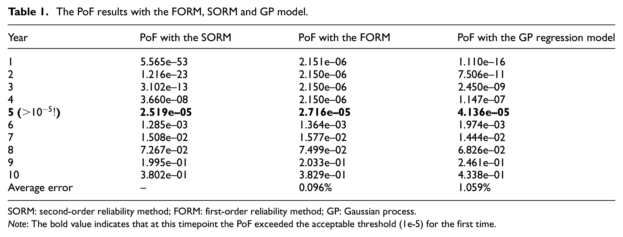
SORM: second-order reliability method; FORM: first-order reliability method; GP: Gaussian process.

Note: The bold value indicates that at this timepoint the PoF exceeded the acceptable threshold (1e-5) for the first time.

Regression with probabilistic layers in TensorFlow probability

In this work, the GP model is implemented with TensorFlow probability (TFP), a library for probabilistic reasoning and statistical analysis. TFP enables the integration of a probabilistic model with deep learning on high-performance hardware (tensor processing unit (TPU), graphics processing unit (GPU)). ²¹ In TFP, various distributions are provided as low-level building blocks, and different probability layers, an inference algorithm, and optimisers are implemented as high-level constructs. The structure of the GP model for probabilistic regression and reliability analysis is shown in Figure 4.

Figure 4.

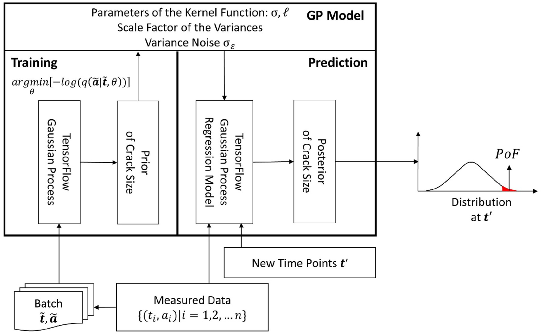
The structure of the GP model with TensorFlow probability.

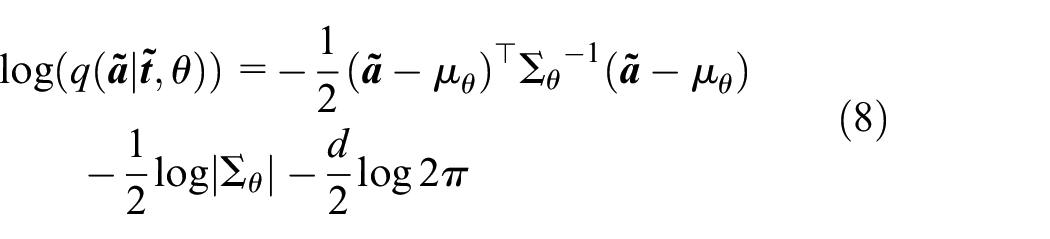
The GP model is trained through a predefined ‘GP’ class, which is an encapsulated high-level application programming interface (API). The model accepts the batched training data as input and outputs the inferred marginal distribution of the GP as the prior. Before training, the parameters of the kernel function, the scale factor of the variance and the noise variance are initialised. With the fed batched data, the parameters of the model are iteratively trained to minimise the negative log-likelihood (see equations (7) and (8)).

The distribution of the crack depth for new time points can be predicted through the class ‘GP Regression Model’, which outputs a posterior from the given measured data, taking the trained parameters in the GP model as the prior. The failure of the probability will be calculated by calling the CDF on the output distributions of the crack depth, with the condition that the crack depth is larger than the critical depth.

In Figure 5, the predicted posterior probability distribution from the GP regression model is shown. The blue points are the ‘measured’ data randomly generated by equation (10) (see section ‘Data preparation and calculation of the PoF based on the FORM/SORM’) for time $\mathit{t}$ . Another set of 400 randomly generated time points $\mathit{t}\prime$ is used to predict the posterior at these time points. The red line represents the predicted mean of the crack depth, and the light grey area is the interval of $\pm 0.1\sigma$ . The mean and the variance of the crack depth also increase over time.

Figure 5.

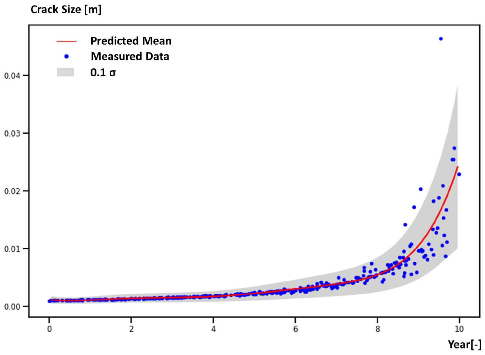
Prediction of the posterior from the GP regression model.

The PoF can be further predicted from year 1 to year 10. The time $\mathit{t}\prime =\{1,2,\dots ,10\}$ is given to the GP regression model to predict the posterior of $\mathit{a}\prime =\{a{\prime }_i|i=1,2,\dots ,10\}$ . The resulting distribution is used to calculate the CDF for $a{\prime }_i\ge a_{\mathrm{critical}}$ .

In this work, the results calculated by the SORM are used as an analytical benchmark. In Figure 6, the predicted PoF (the red points) is compared with the results of the SORM (the blue line). The predicted PoF can approximate the trend of the SORM results. It is difficult to see the difference before year 7 due to the very small value of the PoF. The results are further compared with the log-PoF in Figure 7 between the prediction results (the red line), the FORM results (the orange line) and the SORM results (the blue line). From year 1 to year 4, the prediction results based on the GP model is closer to the results of the SORM than FORM.

Figure 6.

Predicted PoF compared to the results from the SORM.

Figure 7.

Comparison of the log-PoF between the prediction, SORM and FORM results.

The detailed results of the PoF with the GP regression model and analytical methods are presented in Table 1. Both results indicate that an inspection should be planned at the end of the fourth year, since the PoF will exceed the threshold of the PoF ( ${10}^{-5}$ ) at the fifth year. Compared to the PoF calculated by the SORM, the average error of the PoF with the GP regression model is 1.059%, and the average error of the PoF with the FORM is 0.096%.

To verify the developed GP model, it is very common to compare the predicted PoF with analytical results. In this work, the analytic results are calculated from a simplified model that is easy to solve. If the prediction from the GP model coincides with the known results, the model and the results can be interpreted as ‘correct’. However, there is no clear definition of the credibility of the results. For example, the compared results in Table 1 show a large divergence in the magnitude of the PoF during the first 4 years. In this work, the timing that reaches the threshold of the PoF ( ${10}^{-5}$ ) is applied to justify the results, since it is critical for scheduling maintenance activities. For this reason, the results of the GP model are considered credible.

The deviation between the GP regression model and the analytical results becomes significant after year 8. The deviations are caused by the high variance and insufficient information provided by the measured data. This issue should be deeply investigated for developing a whole maintenance plan after the first inspection (e.g. after the fifth year in this case study).

Conclusion and discussions

Findings in this work

In this work, a data-driven approach based on a GP for regression to determine the PoF caused by crack growth in railway axles is developed. For complicated failure modes, it is difficult or even impossible to build a reliable analytical or simulation model before using an analytical approach. The main purpose of this work is to develop an algorithm to infer the distribution of the crack growth from a limited amount of measured data without having to build an underlying model.

After the GP model is trained with the measured data, the distribution of the crack depth can be predicted for any time point. The PoF will be calculated accordingly. Hence, the necessary maintenance activity can be scheduled to ensure that the PoF does not exceed a predefined threshold. The results of the case study show that the determined timing for the first inspection, as well as the PoF, coincides with the known results derived by analytically based approaches. The problems associated with modelling and calibration can be overcome by the data-driven approach. The developed GP model can also serve as a complementary instrument to validate other analytically based approaches or numerical analyses.

Perspectives for further research

The fracture properties of the railway axle are dominantly determined by the crack growth rate and load spectra. Region II (see Figure 3) was already confirmed to fit well through a comparison with the GP model. However, region I and region III should be deeply investigated. Especially, in the early stages of crack growth, it is necessary to determine how the errors in region I affect the predicted results. A 1:1 test bench to the test crack growth with bending and rotating stress was built in CRRC Sifang. Experiments for small-scale specimens and full-scale axles are planned. In the study by Beretta and Carboni, ²² the load interactions under constant and variable amplitudes for different scales are compared. This shows that the effect of the load interaction for full-scale axles is not negligible. The load spectrum should be fully considered in the prediction model.

The effect of parameters on the prediction results needs to be checked. A comparison of the contribution of the parameters on the prediction results will help to understand which parameters are essential for improving the prediction results. The parameters that should be investigated include those for the crack growth model (e.g. the empirical parameters $C$ and $m$ , the SIF, the stress ratio and the geometry factor), the linear material properties (e.g. the elastic modulus and Poisson’s ratio), the residual stresses, the numerical errors and the dimensional tolerances.

As the development and application of the GP are still very active, the issues of tuning the hyper-parameters and model configuration should be addressed. Current development of the GP model is expected so that highly reliable and stable results can be delivered with less manual effort. The accuracy of the model should be further improved, especially for time points with a high variance. Meanwhile, a deep investigation related to the challenge of determining how much available data should be used is required. On one hand, less data will limit the generalisation of the inferred results; on the other hand, more data collected from actual situations increases the computation complexity. In recent years, the variational Gaussian process (VGP) was developed. ²³ It has been proven that the computational complexity of the algorithm can be up to $\mathcal{O}(N^3)$ . In the study by Titsias, ²⁴ a method of using a so-called inducing (pseudo) point instead of the full measured data was developed to reduce the computational effort. This method is also integrated into the optimiser of the TensorFlow VGP layer. The optimiser can find the optimum locations of the inducing points to minimise the negative evidence lower bound (ELBO). ¹⁵ Although the method of inducing points can balance the performance and accuracy, the issue of setting hyper-parameters (e.g. the number of inducing points) should still be investigated and justified. Since the ELBO can only reach a local optimum, the hyper-parameters in the model should be tuned through several rounds of searches. In addition, the choice of the kernel is still questionable. A simplified model with fewer configuration requirements for TFP is expected in the future.

Further research and development will involve developing a maintenance plan for all rounds of inspections in the whole service life. In this work, the probability of crack initiation and the threshold SIF range are not considered with the simplified analytical model. The mechanism of generating an initial crack, the probability of detecting a crack and other stochastic aspects, including the stress and loading during operations, will be studied. The data-driven approach will be examined and validated by other analytically based approaches and numerical analysis. Furthermore, the inference method can be applied to analyse the daily collected data for online detection and diagnosis so that condition-based maintenance for railway axles can be achieved.