Study of concept for hydraulic hose dynamics investigations to enable understanding of the hose fluid–structure interaction behavior

Abstract

Fatigue failure of a hydraulic hose systems, caused by violent vibrations, has become a critical factor creating operational and maintenance cost for the end user of rock drill equipment. Similar behavior is also appearing in, for example, forestry machines. Hoses are used as parts of the energy feeding system in machines such as the ones use for mining and civil construction operations. This work aims to create an understanding of the dynamic behavior of a selected hydraulic hose. The numerical modeling approach selected includes a boundary element method approach in the fluid-elastic analysis of the dynamics of a pressurized hose with conveying fluid. Experimental modal analysis was used to validate the numerical model. Pre-tension and pressure-induced tension were monitored with an in-house-developed strain gauge–based load cell. The analysis and experiments show that a complex coupling, of pure structural bending modes, appears when the hose is subjected to internal flow. Some of the modeshapes show a circular motion of the hose cross sections. As shown in this article, these coupled modes become increasingly sensitive to external or internal excitation with increasing flow rate. To illustrate the strength of the proposed approach, the second part of the work in this article presents a parametric study of hose dynamics for hoses with typical dimensions used in industrial applications. This investigation of how different parameters influence the dynamic characteristics of hydraulic hoses shows, for example, that hose end-support stiffness has a large impact on the stability and dynamic behavior of the hose. A soft support tends to create a static instability–type behavior where the lowest frequency mode frequency decreases to levels close to zero with increasing flow speed. Pre-tension of the hose has a stabilizing effect on the hose dynamics. In the case when the internal pressure of the hydraulic hose does not generate tension of the hose, then the increase or decrease in the internal pressure has limited influence on the hose dynamics: this is at least a conclusion valid in the investigated 100–210 bar pressure range. In addition, a smaller diameter hose is more sensitive than a larger diameter hose, and this is valid as long as the pre-tension is high enough to maintain static stability in the entire flow rate range.

Introduction

Vibration phenomena requiring understanding of fully coupled fluid–structure systems, including fluid-conveying tubes, pipes, and so on, are a dynamic type of problem that have been investigated by numerous authors. The first serious research papers on fluid- conveying tubes, or the pipes vibration phenomena, started to appear in the 1960s, see, for example, Paidoussis.^1,2 The first paper on transient effects of this subject published in the early 1900s was “Theory of Water Hammer” by Allievi. ³ Reviews of the research field were published in 1995 by Tijsseling ⁴ and in 2009 by Wang and Ni. ⁵ As described by Wang and Ni, ⁵ the research of flow-induced vibration of slender structures has been intensified during the past few decades. As stated, this is due to the increasing need for stability and reliability in a broad range of industrial applications: applications ranging from nuclear reactors, heat exchangers, ocean mining pipes, and drill strings as described by, for example, Paidoussis, ⁶ Xia et al., ⁷ and Zhang et al. ⁸ Repeated failures have given evidence to the lack of insight in the physics involved in these types of systems. The phenomena of dynamics related to the internal and or external axial flow fluid–structure interaction (FSI) is a relatively new area of research unlike the case of vibration of slender structures subjected to cross flow. A proposal to address the above type of problem using a fluid-elastic modeling approach is presented. A first effort on applying this method to describe the FSI physics appearing in a high-pressure hydraulic hose system has been made, based on the first author’s past research background, including the development of a so-called generalized aeroelastic methods software described by Hyvärinen. ⁹

Hydraulic hoses with various dimensions are used as energy feeding systems in, for example, rock drill systems. From time to time, these hydraulic hoses are known to start to vibrate violently leading to hose connection failures. These types of failures create production losses and maintenance costs for the drill-rig operator. Traditionally, these problems have been handled by either including an additional accumulator as a filter (as an effort to decrease internal pressure oscillation amplitudes) or by modifying the hose supports to decrease the influence of external vibration sources. In efforts to increase drill speeds and decrease energy consumption on new rock drill developments, system pressure, oil flow rates, and so on, has been changed. This has increased the number of occasions when violent hose vibrations appear, both in the field and in lab environments. The mechanisms and physics behind the vibration phenomena is unknown, leading to a trial-and-error-based approach to resolve the problems. This type of work has been found to be increasingly cumbersome, and thoughts on how to approach these problems have been happening.

In this article, a three-dimensional (3D) type of approach to the fluid-conveying pipe problem is presented. With the fast growth of computer resources in terms of increasing speed and memory size, it has gradually become feasible to model systems with 3D space type models and still get fast results. This enables detailed modeling of hydraulic hose systems including orthotropic behavior for the steel wire reinforced rubber model. The methodology used in this article to describe the linearized unsteady fluid dynamics around a mean steady flow field utilizes a numerical boundary elements method to describe the interface between the fluid and the structure. In addition to the approach being 3D, it also allows the possibility to include all types of modes of motion for the hose; bending as well as modes including cross-sectional shape oscillations.

The purpose of this article is to show how well the 3D behavior of a pressurized hydraulic hose with flowing conveying oil can be modeled and characterized. Also of importance is to show that even the dynamics of stable system can be verified and validated using experimental modal analysis.

The article presents the basic mathematical model selected for the fluid dynamics, followed by a description of how to formulate the so-called fluid-elastic equation of motion and its solution as a non-linear eigenvalue problem. The eigenvalue solution is used to study the characteristics of the dynamics for the investigated coupled system. The results created are frequencies for coupled modes, modeshapes of the coupled modes, and damping requirements for these modes to be neutrally stable. In the following sections, the method used to experimentally evaluate the empty hose structural properties is presented together with a study of a high-pressure oil conveying hose in a laboratory environment. The experimental approach to the investigation of the dynamic characterization of the pressurized hose pressure and flow rate dependence are evaluated. In the “Results and discussion” section, the numerical and experimental results are compared.

To illustrate the type of insight that can be gained using the proposed approach, the second part of the results section presents a parametric study with the goal of creating an increased understanding of the coupled fluid-elastic dynamics for hydraulic hoses of various dimensions used in industrial applications. The parametric study included a study of the dependence on internal pressure, pre-tension, cross section dimensions, and support stiffness. The purpose of the parametric study is to show how different parameters influence the characteristics of the hydraulic hose dynamics using the proposed numerical approach. The results presented include how frequencies of the four first pairs of basic modes depend on the selected parameters. In addition, results presenting the mode sensitivity to excitation are presented. The results created are frequencies for coupled modes, modeshapes of the coupled modes, and damping requirements for these modes to be neutrally stable. An interesting coupled modal behavior is also presented.

System assumption and description

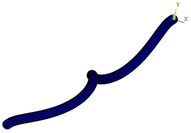
The system that has been investigated is an extension of the system studied by Zhang et al. ¹⁰ It consists of a circular pipe/hose fixed in both ends. In this article, the pure rubber hose has been replaced by a hydraulic hose with a rubber matrix and steel wire core reinforcement. The system is shown schematically in Figure 1.

Figure 1.

Picture of the investigated type of system.

The general assumptions made when setting up the mathematics are here altered to include following:

• A pipe/hose composed of a linear isotropic material.

• A fluid that is incompressible.

• A uniform velocity profile of the fluid.

• A 3D structural model.

• 3D motion.

To study FSI phenomena, one need to solve the fluid-elastic equation of motion (1) also presented as the aeroelastic equation described by Dowell et al. ¹¹

$$M\stackrel{··}{x}(t)+C\stackrel{·}{x}(t)+\mathrm{Kx}(t)=f_a(U_{\infty },\stackrel{·}{x}(t),x(t))+f_e(t)$$

(1)

Most researchers who have published work in the area of pipe conveying fluid dynamic research used the foundation of applied beam type theory for the approximation of equation (1). If external imposed tension, internal damping, gravity, elastic foundation, and pressurization effects are neglected, as described by L Wang and Q Ni, ⁵ the linear equation of motion (2) can be derived

$$\mathrm{EI}\frac{{\partial }^{4}w}{\partial x^4}+M{U}^2\frac{{\partial }^{2}w}{\partial x^2}+2M{U}^2\frac{{\partial }^{2}w}{\partial x\partial t}+(M+m)\frac{{\partial }^{2}w}{\partial x^2}$$

(2)

As seen, the fluid forces are modeled as a plug flow model. Various authors have extended the model to include pre-tension, curvature, and lately also studies of non-linear dynamic phenomena such as amplitude-dependent damping as by Kutin and Bajsic ¹² Until about the end of the 1990s, authors studied phenomena appearing in the time domain as seen in the work by Zhang et al. ¹⁰ A transition into frequency-domain approaches to the problems came during the past couple of decades as, for example, seen in the work by Paidoussis. ¹³ A proposed frequency-domain approach to include cross-sectional modes in the description of the pipe was presented by Kutin and Bajsic ¹² An approach to study the transient response of a slender structure under axial flow by combining structural beam modeling with 3D computational fluid dynamics (CFD) (using a Navier–Stokes solution) has lately been presented by Dressel et al. ¹⁴ The dynamics and stability of a hanging pipe inside a tube using a beam modeling type approach was furthermore presented by Minas and Paidoussis. ¹⁵

As will be illustrated in this article, the suggested approach for modeling of fluid-elastic dynamics is more general than the approaches presented by most authors. The method is for the hose/pipe types of problems to be both efficient and accurate. It considers the majority of the aspects of the appearing phenomena when studying the coupled system.

Modeling approach

The systems modeling of fluid-elastic characteristics include the following three parts: creating a description of the structure dynamics in the Structure Dynamics part, a description of the fluid dynamics in the Fluid Flow Modeling part, and a solution of the eigenvalue problem for the fluid-elastic equation of motion in the Fluid-Elastic Eigenvalue Analysis part. The structure dynamics description is created using modal analysis in a standard finite element method (FEM) program such as ANSYS. ¹⁶ The fluid domain is numerically described with a boundary element method (BEM) model. The flow analysis and the solution of the fluid-elastic equation for the hose dynamic problem in this article has been solved with a tool called LINFLOW, ¹⁷ in which the methods discussed in following section have been implemented.

The following two sections give a description of the selected Fluid Flow Modeling (with discussions on the selected numerical discretization method) and the Fluid-Elastic Eigenvalue Analysis.

Fluid flow modeling

The goal of the fluid modeling is to be able to study unsteady fluid dynamics about some arbitrary mean flow condition. The method also needs to be linear in order to be efficient. The fluid dynamic modeling that satisfies these criteria is the velocity potential model. The basic flow equations in vector notation (as presented by Schettz and Fuchs ¹⁸ ), from which the velocity potential fluid flow equation is derived, are the equation for conservation of mass

$$\frac{\partial \rho }{\partial t}+\nabla \left(\rho \overline{v}\right)=0$$

(3)

and Newton’s second law for a fluid—Navier–Stokes equation

$$\rho \frac{d\overline{v}}{\mathrm{dt}}=-\nabla p+\mu [{\nabla }^2\overline{v}+\frac{1}{3}\nabla (\nabla \overline{v})]+\rho f_e$$

(4)

Consider an approximation in which the viscosity is set to zero, $\mu =0.0$ , hence assuming inviscid flow. In addition, consider a system in which the exterior forces are assumed to be zero $(f_e=0.0)$ , and the flow is assumed to be irrotational, as described in Schettz and Fuchs, ¹⁸ that is

$$\nabla \times \overline{v}=0$$

(5)

The assumption of flow irrotationality means that the velocity field can be expressed as the gradient of a scalar field. As described in Schettz and Fuchs, ¹⁸ this means that the velocity potential $\mathrm{\Phi }$ can be introduced as

$$\overline{v}=\nabla \mathrm{\Phi }$$

(6)

Using the assumptions of mass conservation, an inviscid flow, flow irrotationality, and absence of bulk forces, the flow equations (equation (3)) can be rewritten in terms of the velocity potential field, since the Navier–Stokes equations are specific only to the real (viscous) fluids. This is also presented by Dowell et al. ¹¹

$${\nabla }^2\mathrm{\Phi }-\frac{1}{a^2}[\frac{\partial }{\partial t}(\nabla \mathrm{\Phi }{\nabla }^2\mathrm{\Phi })+\frac{{\partial }^2\varphi }{\partial t^2}+\nabla \left(\frac{\nabla \mathrm{\Phi }\nabla \mathrm{\Phi }}{2}\right)]=0$$

(7)

In the used approach, unsteady flow is studied in the frequency domain, and not in the time domain. In order to study the behavior in the frequency domain, a Fourier transformation is required. Performing the transformation of the above equation in to a frequency domain gives the possibility to derive the following equation for the case of an external flow problem

$${\nabla }^2\mathrm{\Phi }-M^2{(\frac{1}{U_{\infty }}\frac{\partial }{\partial t}+\frac{\partial }{\partial x})}^2\mathrm{\Phi }=0$$

(8)

This equation is also valid for steady flow fields by setting the oscillatory part to zero. The equation now needs to be converted into a form which can be solved by numerical methods, leading to a boundary element formulation.

The BEM can be used for solving a Helmholtz type of equation such as equation (8), see for instance. ¹⁹ The BEM requires the Helmholtz equation, being in differential form, to be transformed into an integral equation. The transformation of the velocity potential equation from differential to integral equations is, for example, found in Dowell et al. ¹¹

The Helmholtz equation is an equation for the flow in the fluid domain. The BEM is based on a reformulation of the flow problem in terms of fields that are defined on the surfaces of the fluid domain. The method is based on the fact that if the field is known on the surfaces of the fluid domain, then there exist equations that describe the field also in the fluid domain. The potential field on the surface of the fluid domain is solved for at a discrete set of points. In the used approach, these are the node points of the boundary element mesh.

The potential field in the fluid domain is defined by surface sources and surface dipole sources that cover the surfaces. The strengths of the surface sources are defined by the fluid velocity normal to the surfaces, while the strength of the dipole sources is defined by the potential field in the node points of the surface. We thus have a closed system of unknowns. The system of coupled equations is summarized by the following questions:

• Given surface sources and surface dipole sources with strengths $q$ and $\mu$ , respectively, what is the potential field in an arbitrary point $r_1$ on the surface?

• How is the surface dipole strength described in terms of the local potential field?

Both of these questions are answered by a derivation leading to equation (9). The first question is the most difficult to answer, while the second question follows as an interpretation of the answer that is found. Figure 2 shows a schematic picture of the modeling considerations. As described by, for example, Dowell et al., ¹¹ the conversion of the differential equations to integral equations is accomplished through a transformation based on Green’s second theorem

$$\underset{V}{\int }({\mathrm{\Phi }}_1{\nabla }^2{\mathrm{\Phi }}_2-{\mathrm{\Phi }}_2{\nabla }^2{\mathrm{\Phi }}_1)\mathrm{dV}=\underset{S}{\int }({\mathrm{\Phi }}_2\frac{\partial {\mathrm{\Phi }}_1}{\partial n}-{\mathrm{\Phi }}_1\frac{\partial {\mathrm{\Phi }}_2}{\partial n})\mathrm{dS}$$

(9)

where ${\mathrm{\Phi }}_1$ and ${\mathrm{\Phi }}_2$ are two arbitrary scalar fields, the left-hand side is the volume integral, and the right-hand side is the surface integral over the bounding surface. The operator is directed in the direction of the outward pointing surface normal. In the current case, the volume under consideration is the fluid domain of the model. Furthermore, it is customary to use a surface normal that points in a direction outward from the structural regions. That is, the normal points into the fluid domain. Introducing the symbol $\overline{n}$ for a normal vector pointing into the fluid domain. The equation that forms the basis for evaluating the coupling between nodes on the boundary (as shown by Brebbia ¹⁹ ) can after some math be defined by

$$\frac{\mathrm{\Omega }({\overline{r}}_1)}{4\pi }{\mathrm{\Phi }}^{*}({\overline{r}}_1)=\frac{1}{4\pi }\underset{S}{\int }[{\mathrm{\Phi }}^{*}(\overline{r})\frac{\partial }{\partial n}-\frac{\partial {\mathrm{\Phi }}^{*}({\overline{r}}_1)}{\partial n}]\frac{e^{-\mathrm{ik}|\overline{r}-{\overline{r}}_1|}}{|\overline{r}-{\overline{r}}_1|}\mathrm{dS}$$

(10)

Figure 2.

Schematics of the boundary element point of view of the fluid–structure interface. This is a pictorial description used to answer the two fundamental questions when using BEM to describe the fluid–structure interface.

An example of the adjustments that are made to the equation when exterior sources is present is here illustrated for external flow problems. In this case, the following term (equation (11)) can be derived and added to the right-hand side of equation (10)

$$U_{\infty }\hat{x}·\overline{R_1}$$

(11)

In the solution of the fluid-elastic problem, the steady and unsteady pressure are used as load, and a linear expression for the pressure as a function of the velocity potential $\mathrm{\Phi }$ is needed. This can be derived from an inviscid, irrotational version of Navier–Stokes equation and the isentropic relationship for the gas. With these assumptions and starting from the momentum equation (4), then the so-called unsteady Bernoulli equation (12) can be derived for fluid oscillations in a steady flow field. This is presented by Dowell et al. ¹¹ and Schettz and Fuchs ¹⁸

$$\frac{\partial \mathrm{\Phi }}{\partial t}+\frac{\overline{v}·\overline{v}}{2}+\underset{p_{\infty }}{\overset{p}{\int }}\frac{1}{\rho }\mathrm{dp}=\frac{U_{\infty }^2}{2}$$

(12)

where the right-hand side follows from the steady flow assumption. By introducing the assumption of compressible isentropic flow, the relationship in equation (13) is formed between the pressure and the fluid density

$$p/{\rho }^{\gamma }=\mathrm{constant}$$

(13)

Also introducing the Mach number $M=U_{\infty }/a$ , and the expression for speed of sound $a^2=\mathrm{dp}/d\rho$ , the Bernoulli equation (14) can be derived as

$$p=p_{\infty }{[1+\frac{\gamma -1}{2}{M}^2(1-\frac{\overline{v}·\overline{v}+2\frac{\partial \mathrm{\Phi }}{\partial t}}{U_{\infty }^2})]}^{\frac{\gamma }{\gamma -1}}$$

(14)

After solving equation (8) for the velocity potential equation, equation (14) gives the steady and unsteady pressure, which is used to evaluate the fluid dynamic load induced by, for example, the motion of a structure.

Fluid-elastic eigenvalue analysis

Problems involving interaction between structural and fluid dynamics can be described by the aeroelastic equation of motion described by Dowell et al. ¹¹ This equation is normally written in terms of modal coordinates that are based on the known/selected structural eigenmodes. The benefit of using modal coordinates is that the number of degrees of freedom in the system is greatly reduced. In aeroelastic applications, only a few of the lowest eigenmodes are normally of interest. The aeroelastic equation of motion (15) expressed in modal coordinates is recognized as the structural dynamic equation as described by Timoshenko et al. ²⁰ with an additional term that includes the aerodynamic matrix (also called the fluid load matrix), which describes the FSI and hence the fluid load induced by participating modes. Assuming harmonic motion, the equation of motion reads

$$-{\omega }^2[M]q(t)+i\omega [C]q+[K]q=[A]q+F$$

(15)

The left-hand side of equation (15) is the modal coordinate space definition of the structure dynamics for a system. Equation (15) is used to solve stability and frequency-domain response problems. The method for finding instabilities is to set the external force to zero and check if there are eigenmodes in the system that are undamped or exponentially growing (hence, have negative damping behavior). The specific methods that are implemented are the V-g method, and the p-k method as, for example, described by Dowell et al. ¹¹ These are methods for finding flow velocities that make the system unstable. They are both iterative methods since the aerodynamic matrix is velocity and frequency-dependent, making the problem non-linear. As described by Dowell et al., ¹¹ the main difference between the two methods is the way iterations are performed. In both methods, a fictitious internal structural damping g is introduced such that the stiffness and damping matrices are written in the form

$$(1+\mathrm{ig})[K]=i\omega [C]+[K]$$

(16)

Solution process

To illustrate the process involved when solving equation (15), the V-g method is here used as an example. In the V-g method, one assumes a value for the critical velocity $V$ and searches for conditions that make the most critical mode unstable. This is an iterative procedure that is repeated until the assumed and obtained values for V are consistent. Hence, the goal with the V-g analysis is to find the velocity at which the most critical fluid-elastic mode requires more damping than what is available in the system in terms of mechanisms such as material hysteresis, friction, viscous induced loss, and any discrete dampers. This critical flow velocity is called the systems flutter speed. It should be noted that in a V-g analysis, one does a solution sweep in a range of the so-called reduced frequency defined as $k=2\pi f_i/v$ , where $f_i$ is the frequency of the ith mode and v is the flow velocity. The eigenvalues from the fluid-elastic analysis contain three parts: frequency, damping requirement for stability, and the velocity index. Each mode is valid only if the user set flow velocity is equal to the velocity index of the mode. In the V-g method approach, only the most critical mode is converged in the search of the flutter speed. This is in contrast to the p-k method, in which each mode is converged at each flow velocity.

Figure 3 shows a flowchart of the modeling approach used in this article including the fluid dynamics modeling, the structure dynamics modeling, and the setup and solution of the non-linear eigenvalue problem for the so-called aeroelastic or fluid-elastic equation of motion (using the V-g method).

Figure 3.

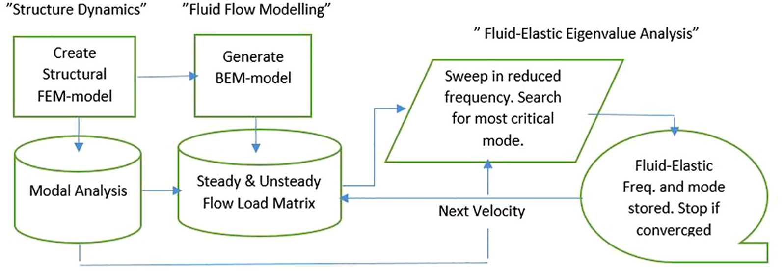
Picture of the non-linear fluid-elastic type analysis process.

The following step-by-step procedure is used when performing the fluid-elastic eigenvalue analysis illustrated by Figure 3:

• The Structure Dynamics part:

1. Create a finite element (FE) model of the structure.

2. Cover the fluid–structure interface with shell-type elements (later used as boundary elements).

3. Define any structural boundary conditions needed.

4. Perform a structural modal (eigenvalue) analysis.

• The Fluid Flow Modeling part:

1. Select the boundary element model.

2. Select the structural eigenvectors to be included in the fluid-elastic analysis.

3. Define the flow conditions to be analyzed.

4. Perform the steady flow analysis at which stability is investigated.

5. Perform an unsteady flow analysis to create the load vector induced by each mode and store it in the [A] matrix of equation (15).

• The Fluid-Elastic Eigenvalue Analysis part:

1. Setup the fluid-elastic equation of motion.

2. Solve the fluid-elastic equation of motion as an eigenvalue problem for a range of reduced frequencies.

3. Find the most critical mode requiring the most damping for stability (check which velocity its damping passes the level of available damping).

4. Adjust the steady flow velocity and re-run from step 4 in the Fluid Flow Modeling part.

5. When the velocity index of the calculated eigenvalue for the most critical mode is equal to the assumed flow velocity, the solution has converge.

6. Perform post-processing of the characteristics creating the critical behavior.

The structure and the fluid domain for the hydraulic hose investigated in this article were numerically discretized with models shown in Figure 4(a) and (b). It should be noted that no mesh or internal grid inside the flow domain is included/needed when numerical discretization using BEM is selected.

Figure 4.

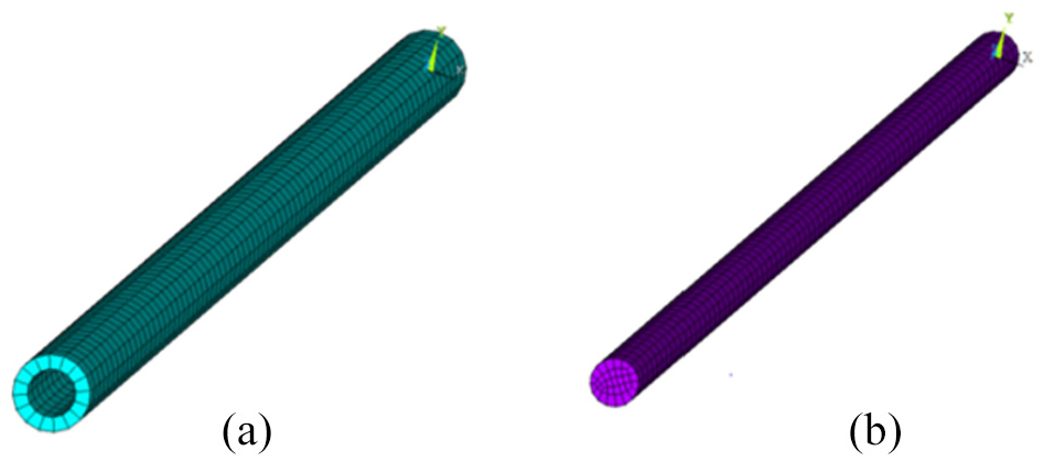
The picture shows (a) a typical FEM used for the structure dynamics part and (b) a typical BEM for fluid flow domain inside the hose.

As illustrated above, several steps need to be taken to finally solve the fluid-elastic equation of motion and evaluate the fluid-elastic characteristics. The process starts by creating a structure FE model and then covering the fluid–structure interface surfaces with boundary elements (modeled by shell-type elements in the pre-processor). The analysis then starts by performing a modal analysis with the structure model. At this stage, the modes to be included in the fluid-elastic analysis (eigenvalues and eigenvectors) are selected and exported to the fluid-elastic solver together with the nodes and elements of the boundary elements. Data for fluid properties and flow conditions are defined together with a selection of the type of analysis that is to be performed. Finally, the solver is started and monitored. The fluid-elastic solver creates results such as fluid-elastic eigenvalues as a function flow velocity and corresponding eigenvectors. Both the eigenvalues and the eigenvectors have complex numbers. The post-processing of the results enables the user to study fluid-elastic mode frequencies and the damping required for the modes to be stable, as a function of flow velocity. In addition, the coupled fluid-elastic motion of the modes can be studied at selected flow conditions.

Material property evaluation

In this work, it was selected to use an experimental approach to evaluate the mechanical properties of the hose. This was important as the hoses were supplied by an external vendor. The experiments require very special facilities for the evaluated properties to be sufficiently accurate. An alternative to this approach would be to create a numerical model of the hose using layered or structure reinforcement type element capabilities available in tools such as ANSYS. Both these alternatives enables creation of a so-called digital twin of the system, enabling tuning of the structural composition of the hose to make its fluid-elastic dynamics behavior stable in the operational envelop of the system in which it is used. This tuning will need to include an optimization process in which the optimum parameters are found.

To evaluate the stiffness properties, static tension, bending, and torsion tests was performed on a selected hydraulic hose. The equivalent material properties (such as Young’s and shear moduli) were obtained, giving a sufficient model to use in the dynamic analysis. Figure 5 shows photographs of the bending and torsion test bench, respectively. The test rig results were used as basis when evaluating the hose stiffness properties used as input in the subsequent numerical analysis. The completed bending and torsional test gave a fairly linear type of behavior, as illustrated from one of the bending tests in Figure 6. With this type of input from the hose tests, and with the cross-sectional dimensions of the hose, it is possible to calculate the properties needed for the numerical analysis of the system behavior. The hydraulic hose conveying oil used in the performed investigation was of “Rockhose” (name of the supplier) type and had following properties: the measured dimensions of the tested hose were length = 1.46 m, outer diameter = 30.7 mm, inner diameter = 19.1 mm, and the density = 2804 kg/m³. The measurements and evaluation described in this section, performed on a few hoses, gave—in average—an Young’s modulus of 111.7 MPa and a Poisson’s ratio of 0.49.

Figure 5.

Test rig facilities used for the evaluation of hose material properties. The bending test rig (left) and the torsion test rig (right).

Figure 6.

The load as a function of deformation during bending in rig. The vertical axle is unit load measured in the machine during hose bending and the horizontal axle shows units of the horizontal motion of the center hose during loading.

Experimental setup and procedures for hose dynamics validation

The experiment was conducted using a closed-loop oil flow experimental facility (see Figure 7). The tested hydraulic hose was mounted on a heavy steel base with a bolt connection on each side. A strain gauge was installed on a cylindrical part of the hollow bolt connection to get the pre-tension force. The stiffness of the installation was checked to make sure that the rig was stiff enough. The goal with the installation was to create a good representation of the typical installation illustrated in Figure 1. A steady oil flow with high pressure was produced with a pump and finally controlled by two control valves located on the upstream and downstream sides of the hose. The flow meter and pressure sensor illustrated in Figure 7 were used to monitor the flow speed and pressure level inside the hydraulic hose. Three oil-pressure levels and four different flow speeds (including a no-flow case) were considered. The test cases considered in this article have flow rates of: 0.0, 5.0, 8.0, and 11.0 m/s at 210 bar pressure. The pre-tension force on the hydraulic hose was kept at the same level (500 N) for all cases. The oil inside the hose was given the following properties: density = 890 kg/m³, speed of sound = 1224 m/s (depending on pressure) given a static pressure of 210 bar, and flow rate range is 5–11 m/s. The impact measurement method was used for experimental modal analysis: 16 positions were successively excited in two directions (the transverse +y, +z directions) with an impact hammer moving with a distance of 0.1 m, as indicated by the numbers in Figure 8. A three-axis accelerometer was glued on the hose surface at the position x = 0.8 m. The signal-to-noise ratio and coherence were checked and only values measured in the y and z directions were included for bending (or possible coupled bending) mode analysis. The measured results were analyzed with PolyMax modal analysis in LMS Test.lab, to get the natural frequencies and modeshapes.

Figure 7.

Closed-loop oil flow experimental facility and impact measurement system.

Figure 8.

Photo of the hose installed in the laboratory. The picture indicates the excitation positions (0–15) and the location of the accelerometer position (8). The used coordinate system has the x-axis along the hose, the y-axis defines the horizontally direction, and the z-axis defines the vertical direction.

Results and discussion

Validation of the proposed approach

The results presented here include a comparison of the experimental modal analysis of the pre-tensioned empty hose with a FEM analysis on a model of the system. This comparison is followed by results from a step-by-step increase in addition to the fluids contribution to the system description. The steps include an analysis with the fluid in rest, followed by an analysis in which the flow rate was gradually increased. The selected flow rate range is a range typically appearing in rock drill systems. Changes in mode frequencies, coupled modal behavior, and the change in damping of the active hose were studied and the results are presented below.

The approach selected was as stated a combination of experimental work and a numerical analysis. The experimental work included a characterization of the structural material properties for the steel wire reinforced rubber hose, numerical analysis of the characteristics of the hose (without oil, with zero flow oil, and with oil in motion), and experimental modal analysis of how the hose dynamics changes depending on which condition it is in. For the work to be successful, it is essential to have data from accurate and carefully performed experiments. The fluid-elastic analysis gives insight into the sensitivity of the hose due to presence of oil at difference flow conditions, but as will be illustrated many aspects influence the total behavior of the hose.

As described above, Young’s and shear moduli were calculated based on pre-static tests, with the assumption that it was sufficient to measure static tension, bending, and torsional stiffness to describe the structure properties of the steel wire reinforced hose. To validate the FE model, a first test was made to compare the model results of a pre-tensioned hose with the corresponding experimental results. Figure 9 shows a comparison between the numerical FE results for the first eight structural and the experimental excitation-based results. The modal structural FE analysis creates pairs of orthogonal bending modes that indicate that the same mode and frequency will be excited independent of the excitation direction; which transvers, mode/modes that will be excited only depends on the frequency of excitation and damping in the system though some of the neighboring modes may also be excited. The first four lowest frequency modeshapes, with frequencies presented in Figure 9, are shown in Figure 10(a)–(d).

Figure 9.

Experimental and calculated frequencies for the eight first modes which illustrate the agreement achieved between the modal results for the empty hose.

Figure 10.

The shape of the 8.4-Hz first mode pair (a), the shape of the 18-Hz second mode pair (b), The shape of the 58-Hz third mode pair (c), the shape of the 77-Hz fourth mode pair (d).

When viewing the modal motion of these structural modes, the motion remains in one plane. This will not always be the case when including the flowing medium into the system, due to fluid-elastic coupling (as will be show below for the fluid-elastic cases).

When adding the pressurized oil into the hose (without mass flow through the hose), the results in Table 1 are obtained. The measured pre-tension changes from 500 N tension of load in the load cell to about 2100 N (compression in the load cell is included in the experimental setup).

Table 1.

Comparing numerical and experimental mode frequencies for the first five modes (the hose is pre-tensioned with oil at zero flow rate).

Fluid-elastic mode number	Numerical (Hz)	Experimental (Hz)	Difference %
1	13.91	13.7	1.5
2	28.42	29.2	2.7
3	44.11	47.0	6.1
4	61.51	68.6	10.3
5	81.07	94.8	14.4

As described in the “Fluid-elastic eigenvalue analysis” section, the solution of the non-linear eigenvalue problem requires an iterative procedure in order to converge the results for each mode at each flow condition. Having converged each mode at each flow rate for a specific flow condition enables the creation of diagrams on how eigenfrequencies depend on flow rate and the damping required for each mode to be neutrally stable. These diagrams are shown in Figures 11 and 12 for the 210 bar pressure level. The zero flow rate in Table 1 corresponds to the zero flow rate points in Figure 11.

Figure 11.

Fluid-elastic mode frequencies in Hz for the first five modes as a function of velocity in m/s.

Figure 12.

Damping requirement (in relative damping) for neutral stability to the first five modes as a function of velocity in m/s.

From Figure 12, it can be interpreted that with increasing velocity, the hose shows a gradual increase in sensitivity to external or internal excitation. Also, the higher frequency modes start to show an increasing rate of excitation sensitivity at 4–6 m/s flow speed. The fluid-elastic modeshapes for the four lowest frequency modes is presented in Figure 13(a)–(d). The views in these figures show the fluid-elastic mode during one motion cycle presenting it as a composition of 10 frames. When viewing a cross section of the hose at a maximum amplitude location, a circular or elliptical type of motion appears, which varies depending on the studied mode.

Figure 13.

(a) The shape of the first 13-Hz fluid-elastic mode, (b) the shape of the second 26-Hz fluid-elastic mode (c) the shape of the third 43-Hz fluid-elastic mode and (d) the shape of the fourth 58-Hz fluid-elastic mode.

Taking a closer look at the frequency behavior presented in Figure 11, Figure 14 shows that the coupled mode frequency for mode 3 (the 43 Hz model in Figure 11) is slowly decreasing with flow velocity, which is the same type of behavior as showed by YL Zhang et al. ¹⁰ for a pure rubber hose. If the velocity range had been increased, a more pronounced frequency drop would appear. The flow velocity range was kept within the range used in typical rock drill systems in which the hose is the energy feeding part. All the investigated modes show similar behavior in the investigated flow range.

Figure 14.

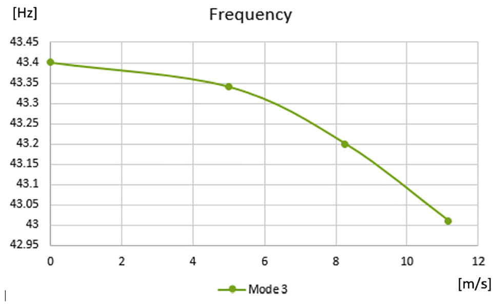
Fluid-elastic mode frequencies for the mode 3 as a function of velocity in m/s.

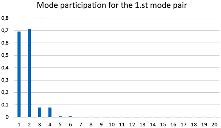
An additional result that is available when using the suggested approach is the modal behavior of the fluid-elastic coupled modes. This result is obtained by viewing the eigenvector corresponding to a specific eigenvalue. The eigenvector describes how the real structural modes shall be combined to create the fluid-elastic mode. As an example, a result achieved with 210 bar and 8 m/s flow is regarded. For this condition, Figure 15 shows how the eight first structural modes (out of the 20 modes included in this case) participate to describe fluid-elastic mode number 3. In general, all selected structural modes participate in the description of a specific fluid-elastic mode, but as seen in Figure 15, a complex combination of modes 5 and 6 is dominating the description of fluid-elastic mode 3. Figure 15 shows the size of the participation factors for the participating modes and the results in table in Figure 15 shows that there is a non-zero phase relationship between the modes. Using the eigenvector for fluid-elastic mode 3 and viewing the fluid-elastic mode 1 motion cycle (presented it as a composition of frames), the results in Figure 13(c) are obtained. The figure illustrates the fluid-domain model motion, showing that if one views a cross-sectional plane through the hose, then an elliptic motion of the cross section is seen.

Figure 15.

Amplitude of modal participation for included structural modes describing the third 41-Hz fluid-elastic mode.

In the following, the results from the 210 bar and 8 m/s flow rate case is studied, and the results from the experimental work is again compared with corresponding results from the numerical analysis. Table 2 shows a level of agreement similar to the ones found in the pure structural case. The reason for the shift sign in the Difference column, that is, the difference between the numerical and the experimental results, is due to that two error sources involved: the first is an overestimation of the pre-tension (evaluated from the experimental load cell) in the numerical analysis and second is that the assumed boundary conditions and isotropic material assumption error tend to increase with frequency, creating a gradually increasing error.

Table 2.

Experimental and calculated fluid-elastic dynamics with 8 m/s flow.

Fluid-elastic mode number	Numerical (Hz)	Experimental (Hz)	Difference %
1	12.8	12.6	+1.6
2	26.4	26.1	+1.1
3	41.2	42.2	–2.4
4	57.9	60.4	–4.1
5	76.8	81.7	–6.0

An interesting question arise; will the fluid-elastic (FSI) modal behavior appear experimentally if a one-directional excitation/hammering is applied on the hose? The answer is yes, as seen in Figure 16(a) for the first 12.8 Hz mode, the excitation direction mode will naturally couple with its orthogonal companion mode through the fluid-elastic coupling. The corresponding 12.6 Hz calculated mode is seen in Figure 16(b). The figures were created in the same way as described for Figure 13(a)–(d).

Figure 16.

(a) The modeshape of the experimental 12.8-Hz mode and (b) the modeshape of the numerically calculated 12.6-Hz mode.

The experimental work shows significant decrease in system damping when pressurizing the hose. The damping decreases even more with increase in the flow rate, which is in line with the numerical observations. Figure 17 shows the behavior for the 210 bar case. Figure 17 shows that mode 1 with 12 Hz frequency (see Table 2) has a damping level of about 2.4% when no oil is present and about 0.9% at 8 m/s flow rate. As seen, the rate of decrease in the available damping increases with the frequency of the mode. It should be noted that the first data point on the curve for each mode in Figure 17 is the damping level for the empty hose.

Figure 17.

Experimental modal damping for the first lowest frequency modes.

For a real-world installation, two types of scenarios may appear: either, the system designer has questions of whether the installation at hand has sensitive dynamic behavior at the operational conditions for the system, or why the hose in a current installation (including its mounts) wearing out fast. Both of these questions may be answered by stepping through and converging the properties for all modes appearing in the excitation frequency spectrum that the hose is subjected to. As an illustration, a 4-m-long, 3/4-inch hose subjected to excitation up to 70 Hz was investigated, and the diagram for damping requirement as a function of frequency was extracted. Figure 18 shows the diagram that was created, and it clearly shows that the hose in this case is most sensitive to excitation at about 62 Hz. The next step is to investigate what type of mode the 62 Hz mode is. This can be conducted by plotting and animating the most sensitive mode. Figure 19 shows that this mode has a combined tension/compression and radial expansion–type behavior. Using this hose installation in a system created extensive wear of one of the support structures as shown in Figure 20. The experimental evaluation also confirmed that tension compression type motion was causing the wear. Hence, the used method enables understanding of the reasons for the problem and the possibility to evaluate what changes that could be implemented to remove the behavior. One example of improvement would be to replace the hose with one that has the critical mode type outside the operational frequency range.

Figure 18.

Dynamic sensitivity of a 4-m-long, 3/4-inch hose.

Figure 19.

Illustration of the mode that is most sensitive to excitation at the operational conditions of the 4-m-long, 3/4-inch hose.

Figure 20.

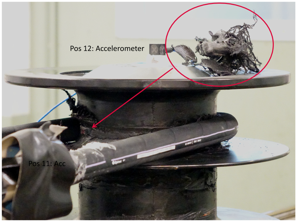
The picture shows the wear of one the of the end-supports for the 4-m-long, 3/4-inch hose. The condition shown is appearing after a short time of usage. The picture shows the drum around which the hose is tensioned. The highlighted material in the upper right part of the picture is material that has eroded from the drum surface.

Parametric study of hose dynamics

This section presents a parametric study utilizing the approach demonstrated in this article. The performed investigation included hoses that had following properties: the dimensions of the hoses included in the study were $1/2$ , $3/4$ , and 1.0 inch (inner hose diameter). The nominal hose length used was 4.0 m. As described above, Young’s and shear moduli of each individual dimension were calculated based on the static tests, with the assumption that it was sufficient to measure static tension, bending, and torsional stiffness to describe the structure properties of the steel wire reinforced hose. The first 4 lowest structural modeshapes, and frequencies are shown in Figure 21(a)–(d).

Figure 21.

The shape of the 8.4-Hz first mode pair (a), the shape of the 18-Hz second mode pair (b), the shape of the 58-Hz third mode pair (c), and the shape of the 77-Hz fourth mode pair (d).

The structure model and modal information of the type described above are used as input in the fluid-elastic investigation presented in this article. Following fluid-elastic studies was made in this work:

1. Study of influence of end-support stiffness on the hose dynamics.

2. Study of influence by pre-tension level.

3. Study of static pressure level influence on the hose dynamics.

4. Study of influence of hose dimensions (0.5–1.0 in diameter) on the hose dynamics.

In the following, four numbered subsections the results are presented, as diagrams of how the first four fluid-elastic transverse bending mode frequencies change with flow velocity, and how the corresponding damping required for neutral stability changes with flow velocity for each case. To interpret the diagrams presented in this section, the following definitions need to be kept in mind:

• A mode becomes statically unstable if/when the frequency of the mode drops to zero.

• A mode becomes dynamically unstable if/when the damping requirement for neutral stability exceeds the amount of damping available in the system.

• Negative damping requirement level is an additional fluid-elastic inviscid type of damping that appears. Hence, the damping requirement is a description of how much energy is transferred in or out of the system.

Study of influence of end-support stiffness on hose dynamics

When considering the first transverse bending mode at around 1.0 Hz for the first series of results, the hose behavior when the end-support stiffness is varied is shown in the diagrams below. In this case, a 0.0 N pre-tension was used. Two support stiffness levels was investigated $\mathrm{Ksup}=1.0\mathrm{E}2\mathrm{N}/\mathrm{m}$ and $\mathrm{Ksup}=1.0\mathrm{E}5\mathrm{N}/\mathrm{m}$ The stiffness influence on the dynamic characteristics for the softer case, starting at about 0.9 Hz for zero flow velocity, shows a gradually increasing stabilization with flow rate up to about 6.5 m/s, while at a higher flow rate of about 10 m/s, it shows static instability type of behavior. The stiffer support case shows higher sensitivity to excitation at a lower flow rate and becomes statically unstable at slightly higher flow rate as seen in Figure 22. The dynamic stability behavior of the first mode for the softer support case shows stabilizing behavior at the lower flow rates and unstable behavior at the highest flow rate (the damping requirement is at same level as for the stiff case) as shown in Figure 23.

Figure 22.

Fluid-elastic frequency diagram for the first transverse bending mode. The stiffer support mode (red curve) shows slightly higher stability than the softer support case.

Figure 23.

Fluid-elastic damping diagram for the first transverse bending mode. The softer support case (red curve) shows dynamically stabilizing behavior at the lower flow rate range and the stiffer support version shows small but destabilizing behavior.

Figure 24 shows the modeshape of the presented mode. As seen, the soft support end shows non-zero motion, which is known to cause static instability–type behavior as discussed by Kutin and Bajsic. ¹²

Figure 24.

Fluid-elastic mode corresponding to Figures 22 and 23. The soft support end to the right shows non-zero motion which is known to cause static instability type behavior. Red color indicates highest amplitude motion and blue indicates smallest amplitude motion.

Study of influence by pre-tension level

The dynamic hose characteristics are dependent on pre-tension level. An investigation of the change in characteristics, of the first transverse bending mode, when pre-tension is increased is presented. A pre-tension of 1400 N is compared with the 0.0 N pre-tension case. The frequency of the mode increases to about 6 Hz, and the pre-tension shifts the static instability to a much higher flow rate as shown in Figure 25.

Figure 25.

The fluid-elastic frequency diagram (left) and the damping requirement diagram for neutral stability for the first transverse bending mode when comparing behavior for the $0.0\mathrm{N}$ pre-tension case (blue colored curve) with a $1400\mathrm{N}$ pre-tension case.

Study of static pressure level influence on the hose dynamics

Both the numerical analysis and the experimental work show that a pressure increase has a stabilizing effect on the fluid-elastic dynamics, that is, the hose become less sensitive to flow rate related dynamics. The problem is that static pressure influences two features of the problem the pre-tension and the fluid dynamics. In this investigation, the pre-tension is kept constant and the fluid pressure is increased. This will only be possible if the steel wire reinforcement orientation in the hose is accurately controlled so that inner pressure does not create pre-tension. A pre-tension of 700 N was selected for this study. The results in Figure 26 show that a shift from $100$ to $210\mathrm{bar}$ only has a limited impact on the hose behavior. The frequencies of the modes in Figure 26 range from about $2-15\mathrm{Hz}$ .

Figure 26.

Damping requirement diagram for neutral stability for the first five transverse bending modes at $700\mathrm{N}$ pre-tension when comparing the behavior for the $100\mathrm{bar}$ case with a $210\mathrm{bar}$ case.

Study of influence of hose dimensions (0.5–1.0 inch diameter) on hose dynamics

A model which was fixed at both ends was used to investigate the dynamics of the 4.0-m-long hose change when the inner diameter was varied from $0.5-1.0\mathrm{inch}$ . The structural stiffness data for the $1/2$ , $3/4$ , and $1.0\mathrm{inch}$ inner diameter hoses was measured experimentally. The stiffness information was transferred into the numerical model as described earlier in this article. The pre-tension was kept at a low level $130\mathrm{N}$ .

Figure 27 shows that a dimension size increase has a stabilizing effect, but if the pre-tension level is too low, the larger diameter hose has a tendency to become vibration sensitive with increasing flow rate (this is creating so-called statically unstable conditions for the lowest frequency mode). To finally illustrate the type of modes that appear when the flow speed is increased in a hydraulic hose, the behavior for the $3/4\mathrm{inch}$ hose at 210 bar pressure with a 20 m/s flow rate through the hose is presented. Figure 28 shows the amplitude of the complex mode participation factors creating the first fluid-elastic mode, and the frequency of the mode is 0.51 Hz.

Figure 27.

The damping requirement and frequency diagrams for the first five transverse bending modes for the $1/2$ , $3/4$ , and $1.0\mathrm{inch}$ inner diameter hoses.

Figure 28.

Mode participation factors for the first pair of fluid-elastic modes.

The modeshape of the first fluid-elastic mode pair is shown in Figure 29. When focusing on one cross section of the hose during the mode motion, it has a circular type of motion.

Figure 29.

The modeshape of first fluid-elastic modes (the cross section of the hose has a circular motion during animation due to modal coupling).

Figure 30 shows the amplitude of the complex mode participation factors creating the second fluid-elastic mode at 210 bar pressure for the $3/4\mathrm{inch}$ hose, with a 20 m/s flow rate through the hose. The frequency of the mode is 1.45 Hz.

Figure 30.

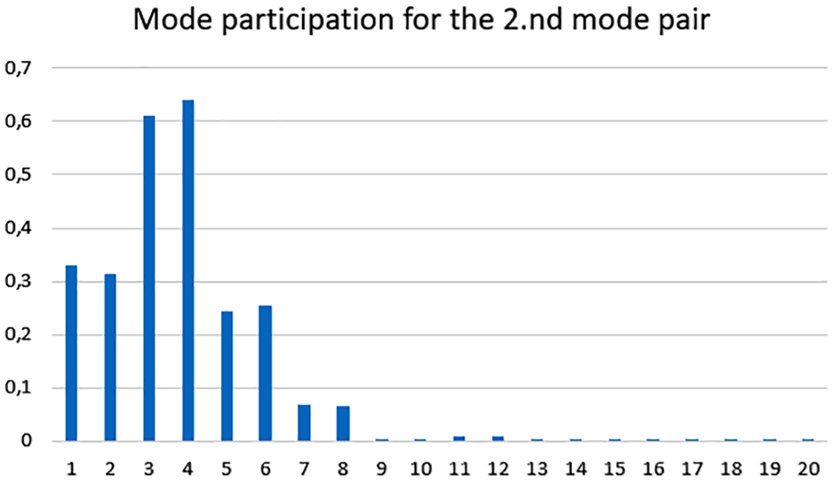
Mode participation factors for the second pair of fluid-elastic modes.

The modeshape of the second fluid-elastic mode pair is shown in Figure 31. As seen, several of the hose structural modes participate and a more complex motion is created. When focusing on one cross section of the hose during the mode motion, it has a circular or elliptic type of motion.

Figure 31.

The modeshape of second fluid-elastic modes (the cross section of the hose has a circular motion during animation due to modal coupling).

Figure 32 shows the amplitude of the complex mode participation factors creating the third fluid-elastic mode at 210 bar pressure for the $3/4\mathrm{inch}$ hose, with a 20 m/s flow rate through the hose. The frequency of the mode is 2.77 Hz.

Figure 32.

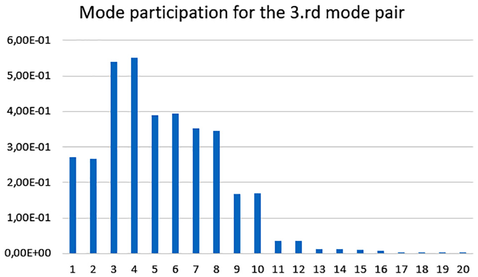
Mode participation factors for the third fluid-elastic modes.

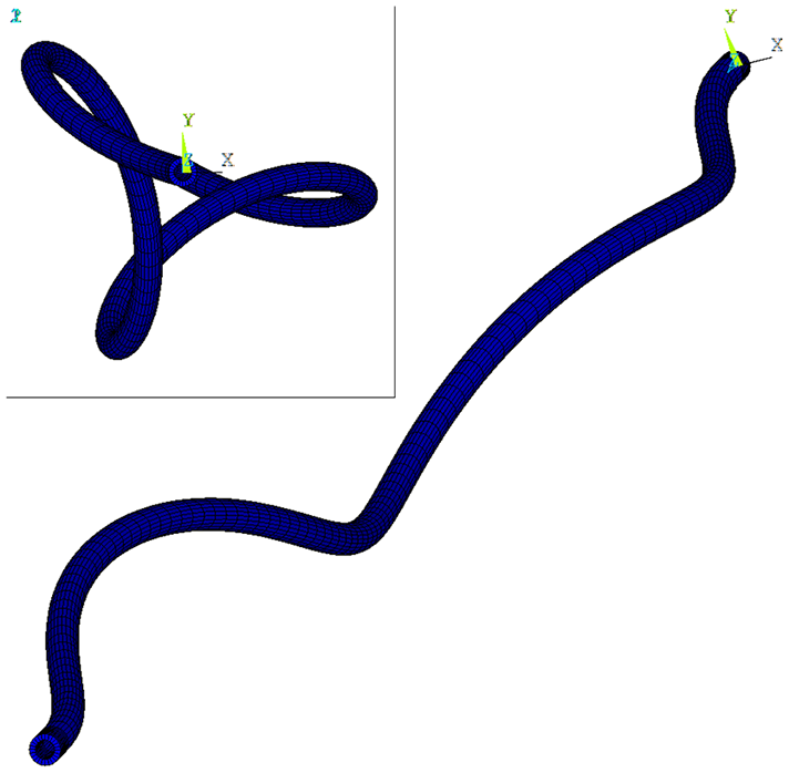
The modeshape of the third fluid-elastic mode pair is shown in Figure 33. The upper left picture is a view of the mode looking into the flow direction. As seen, an increasing number of the hose structural modes participate and a more complex motion is once again created. When focusing on one cross section of the hose during the mode motion, it has a circular or elliptic type of motion.

Figure 33.

The modeshape of third fluid-elastic mode (the cross section of the hose has a circular motion during animation due to modal coupling).

Figure 34 shows the amplitude of the complex mode participation factors creating the fourth fluid-elastic mode at 210 bar pressure for the $3/4\mathrm{inch}$ hose, with a 20 m/s flow rate through the hose. The frequency of the mode is 5.14 Hz.

Figure 34.

Mode participation factors for the fourth fluid-elastic mode.

The modeshape of the fourth fluid-elastic mode pair is shown in Figure 35. As seen, an increasing number of the hose structural mode participate an increasingly more complex motion is created. This mode shows a wave propagation type of behavior. When focusing on one cross section of the hose during the mode motion, it also has an elliptic type of motion.

Figure 35.

The modeshape of fourth fluid-elastic mode (the mode shows a wave propagation type of behavior).

Conclusion

A combined FE/boundary element modeling approach earlier developed for aeroelastic applications has been tested on a pressurized hydraulic oil hose that was “fixed” at both ends. In addition to validating, the two modeling questions were answered: first, is it sufficient to use tension, bending, and torsion test to extract stiffness properties of for the steel wire reinforced hose?, and second, is it by using an experimental modal hammering based technique possible to excite the fluid-elastic coupled modes?. The results show that the answers to these questions is yes. The results also show that using the suggested approach will most likely enable a great insight into the dynamics involved creating violent vibrations on hydraulic hose systems, feeding energy to, for example, rock drills on rock drill rigs. To illustrate the type of insight that can be gained using the proposed approach, a separate study was presented. This study was an investigation into how different parameters influence the dynamic characteristics of hydraulic hoses, and it was shown that

• Hose end-support stiffness has a large impact on the stability and dynamic behavior of the hose. A soft support tends to create a static instability type of behavior where the frequency of the first mode decreases to levels close to zero with increase in the flow speed.

• Pre-tension has a stabilizing effect on the hose dynamics.

• In the case when the internal pressure of the hydraulic hose does not generate tension of the hose, then the increase or decrease in the internal pressure has limited influence on the hose dynamics. This is at least a conclusion valid in the investigated 100–210 bar range.

• A smaller diameter hose is more sensitive than a larger diameter hose. This is valid as long as the pre-tension is high enough to maintain static stability in the entire flow rate operation range.