
Abstract
Viscous flow over a porous and stretching (shrinking) surface of an arbitrary shape is investigated in this article. New dimensions of the modeled problem are explored through the existing mathematical analogies in such a way that it generalizes the classical simulations. The latest principles provide a framework for unification, and the consolidated approach modifies the classical formulations. A realistic model is presented with new features in order to explain variety of previous observations on the said problems. As a result, new and upgraded version of the problem is appeared for all such models. A set of new, unusual, and generalized transformations is formed for the velocity components and similarity variables. The modified transformations are equipped with generalized stretching (shrinking), porous velocities, and surface geometry. The boundary layer governing equations are reduced into a set of ordinary differential equations (ODEs) by using the unification procedure and technique. The set of ODEs has two unknown functions f and g. The modeled equations have five different parameters, which help us to reduce the problem into all previous formulations. The problem is solved analytically and numerically. The current simulation and its solutions are also compared with existing models for specific value of the parameters, and excellent agreement is found between the solutions.
Introduction
The present progress regarding fluid flow over a porous and stretching (shrinking) sheet is incremental and substantial. The physical models of fluid flow have profound applications in extrusion processes and metal industries.1–3 Notable achievements and investigations have been made, and the researchers are recorded new observations regarding such models. Sakiadis 4 studied boundary layer flow of an incompressible fluid over a continuous stretching sheet moving with a constant speed. The next significant and analytical study was presented for the variable stretching velocity by Crane. 5 A new similarity solution is explored by Banks 6 for a boundary layer flow due to stretching surface, and he provided new analytical and numerical solutions to the problem. Moreover, he also presented some special non-similar solutions of the flow problem. Later on, the Eigen solutions of boundary layer flow over stretching sheets have been examined and investigated by Banks and Zaturska. 7 Flow and heat transfer over a continuous linearly stretched sheet with variable surface temperature have been discussed by Grubka and Bobba 8 and solved the problem by using special Kummer’s function. The reference papers are mainly concerned about similarity solutions of viscous fluid flows over a porous stretching (shrinking) sheet.9–12 McLeod and Rajagopal 13 examined the unique solution of Navier–Stokes equation for a viscous flow over a stretching sheet. Chang et al. 14 and Lawrence et al. 15 investigated the multiple solutions of a non-Newtonian fluid flows over a stretching sheet. Recently, lot of works have been carried out by many researchers to model and solve the problems of fluid flow related to stretching (shrinking) over a sheet of an arbitrary shape in Newtonian and non-Newtonian fluids.16–24 This section is strengthened by citing latest research work from the literature into it. In these research articles, nano and micropolar fluid models are investigated for both Newtonian and non-Newtonian fluids over a stretching sheet. The convective flow of nano fluids is analyzed in some of the studies,25–31 and interesting results have been pursued for flow and heat transport in such special situations. A model problem of viscous flow and heat transfer is studied over a stretching sheet for passive control of nano particles on surface of a thin layer of fluid. 25 Later on, this model is further extended for non-Newtonian fluids. 26 Other researchers27–31 investigated the flow, heat, and mass transfer in fluids maintained over a stretching sheet. The important application of boundary layer flow is further enhanced in some works,32–36 and they discussed steady flow with magnetohydrodynamic (MHD) effects, unsteady flow and heat transfer with MHD effects, unsteady mixed convection flow with magnetic effect, and unsteady natural convection flow with MHD effects for micropolar fluid. The study of MHD thermosolutal Marangoni boundary layer flow without convection is discussed by Magyari, 37 and the study of fluid flow with convection over a flat surface in the presence of heat generation or absorption effects is discussed by Chamkha. 38 Moreover, MHD flows of chemically reactive species of micropolar fluid in the presence of heat generation or absorption are investigated in the works of Khedr et al. 39 and Damseh et al. 40 On the contrary, numerous studies have been carried out to improve the thermal conductivity of fluids by including nano/micro or large-sized particle materials into it. A comprehensive survey of all such cases has been completed by Chamkha.41,42 Chamkha et al. 41 found the effects of stretching surfaces on three-dimensional micropolar fluids. The mathematical simulations in Chamkha et al. 41 offer the insights of wall-driven flows into the mechanisms studied so far. Chamkha et al. 42 investigated the effects of uniform lateral mass flux on non-Darcy natural convection boundary layer flow of a non-Newtonian fluid over a permeable vertical cone embedded in a porous medium filled with nano fluid. Note that this investigation is completed by considering the Brownian motion and the inputs of thermophoresis. Stretching (shrinking) problems are attempted by many researchers such that they transformed the governing non-linear boundary value problem into self-similar form, and later on they found either exact or the numerical solutions of the simplified problem. There are few stretching (shrinking) problems for which exact analytical solution are known.43,44
In this article, the results of those classical models are recovered which describe fluid flow over a variable (uniform), stretched (shrunk), and porous (variable and uniform) sheet of variable thickness. The problem is formulated in terms of the continuity equation and boundary layer momentum equation with generalized boundary conditions. The boundary conditions are taken on stretched (shrunk) and porous (injection/suction) surface of variable thickness. A set of generalized and unusual similarity transformations is formed for the velocity components and similarity variable. By means of the transformation, the governing partial differential equations (PDEs) together with boundary conditions are converted into a set of coupled boundary value problems. The last system has two ordinary differential equations (ODEs) in two unknown functions, which are the representatives of velocity components. The new modeled equations are matched with some of the studies4,10,16–24 for fixed value of parameters involved in the problem, and details of the comparison are shown in tables and graphs. New exact, numerical, and power series solutions of the modeled problem are attempted. The approximate solutions are compared with the exact and numerical solutions, and excellent agreement is found among them. Moreover, the solutions are also compared with the published results for fixed value of the parameters, and these observations are presented in different tables and figures. Velocity and shear stress profiles are graphed for different values of all these parameters, and interesting results have been produced and discussed. New profiles are also added for the sake of comparison with classical results. The comprehensive graphs of new and classical predications ensure the difference between the two.
Problem formulation
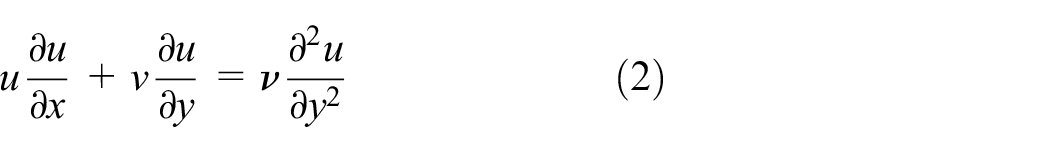
Here, we assumed two-dimensional, steady, and laminar flow of an incompressible viscous fluid, and the flow is maintained over a stretched (shrunk) and porous sheet. The sheet of variable thickness is porous, and the porous velocity is variable, whereas the stretching/shrinking velocity is also non-uniform. Moreover, the ambient fluid is at rest. The following governing equations are taken for the modeled problem, which include continuity and boundary layer momentum equation

It is customary to define the no-slip condition at fluid–solid interface. Therefore, the velocity components are considered on stretched (shrunk) and porous surface,


where
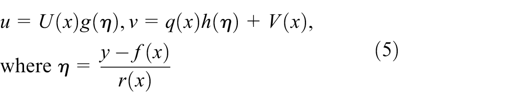
The new variables in equation (5) are formed on the basis of analogies used in the study of Kármán 45 and substituted into the governing PDEs (1) and (2), and we get the following ODEs


The boundary conditions in equations (3) and (4) (see Figure 1) are reduced as

where the prime denotes differentiation with respect to

Geometry of the physical model under consideration and its coordinates.
Solutions of the problem
In this section, we present the exact solution for specific value of parameters involved in the problem. A series solution coupled with Padé approximation is also found for general value of parameters. The series solution is compared with the exact and numerical solutions of the problem. The series solution is exactly matched with the other two solutions, and accuracy of the solutions is established. The exact solutions of the highly non-linear Navier–Stokes equations are few; therefore, in some cases, the closed form solutions of the governing equations are found and these recommended solutions are cited by many researchers. Moreover, the numerical solutions or computer’s generated solutions are usually compared with the closed form solutions (exact solutions) in order to determine their accuracy and establish their correctness. So these exact solutions are meaningful and applicable, and work as a baseline solution by which one can validate the numerical results. This is the most reasonable argument to compare the computer-generated solutions with the closed form solutions. The exact solutions cannot be formed for all situations, and only special cases are known (came into being) for which such solutions can be found. On the other hand, the classical exact solutions of the popular modeled problems Crane 5 , Banks 6 and Grubka & Bobba 8 are highly cited by many researchers for the comparison of the numerical/approximate solution of their problems. The main objective of the exact solution is to facilitate the computer-generated approximate solutions in the form of comparison. Note that a set of classical solutions is also retrieved from these solutions. In this section, we have presented four different closed form solutions of boundary value problem in equations (6)–(8). These solutions are in the form of rational, hyperbolic, and exponential functions.
Exact solution
Case I (when
The closed form solution, given below, is in the form of rational functions and clearly asymptotic in nature. This solution is not valid for all choices of the value of parameters. Therefore, some constraints have been imposed on the governing parameters. The denominator of these rational functions cannot be zero, so we need to avoid all those values of the parameters for which the denominator vanishes. The boundary value problem in equations (6)–(8) has a closed form solution for
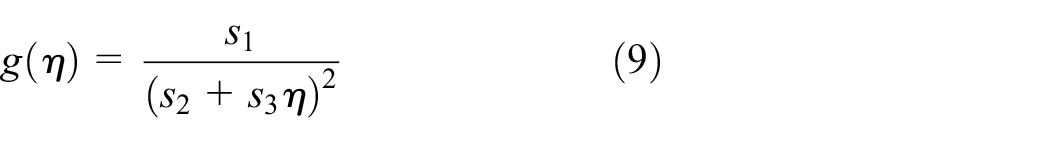

where
Case II (when
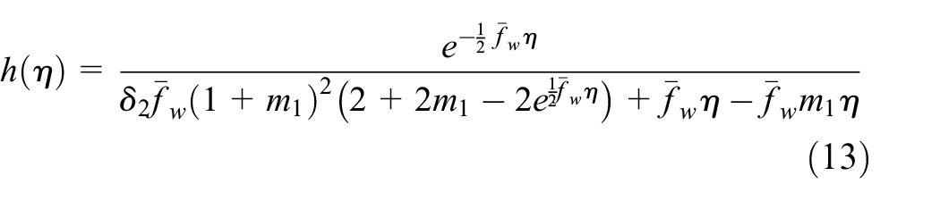
Another closed form solution of the boundary value problem in equations (6)–(8) is found by hit and trial method, and it has the following form


Case III
For

where
Case IV
A fourth solution of equations (6)–(8) is found for special values of the parameters, that is,


where
Power series solution
The laborious power series solution of equations (6)–(8) is presented here. Notice that the unknown functions


where the coefficients
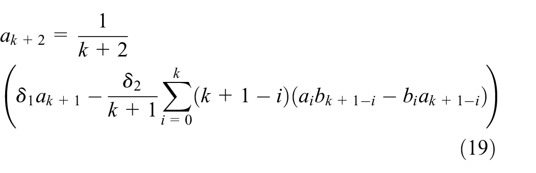
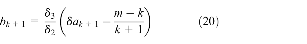
where
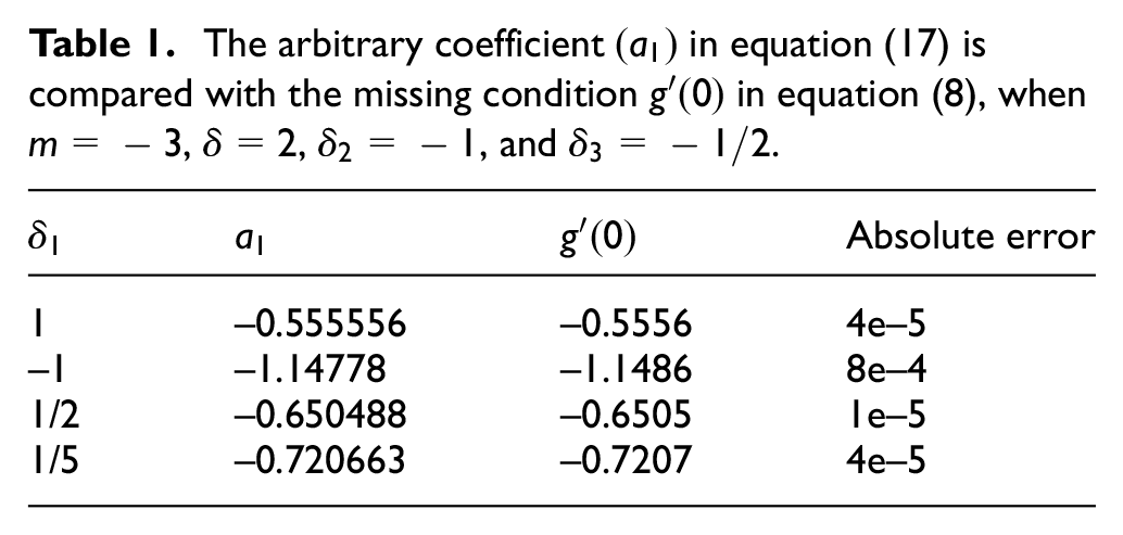
The arbitrary coefficient
Comparison of the power series solution with a numerical solution
The power series solution in equations (17) and (18) and numerical solution of equations (6)–(8) are compared in Table 2 for different values of
Power series solution in equation (17) is compared with the numerical solution of equations (6)–(8) for


Axial velocity (normalized) is graphed against
Comparison of the current model and its solutions with literature
The current simulation is compared with the published models for proper and fixed value of the parameters. The unknown functions of the current model are replaced by the respective functions used in the published problems. In addition, we recovered the previous models of the earlier studies4,10,16–24 such that the parameters
The current model in equations (6)–(8) is compared with published papers.


Critical values for different ranges of parameters when


Axial velocity (normalized) is graphed against
Different values of parameters are fixed for each profile in Figure 3.

Discussion
In this section, the field properties are elaborated for fixed value of parameters appeared in modeled equations (6)–(8). The effects of all these parameters are seen on the axial and normal velocity components
Shear stress
The shear stress due to moving fluid can be obtained from the following Newton’s law of viscosity
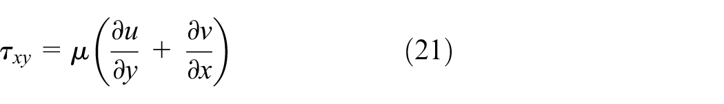
In view of equation (5), equation (21) becomes

The shear stress at the surface of the sheet (skin friction) is modified and non-dimensionalized, which is presented by the following relation

where
Figure 4 shows the profiles of skin friction coefficients
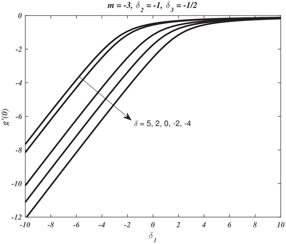
Skin fraction coefficient is plotted against

Skin fraction coefficient is plotted against
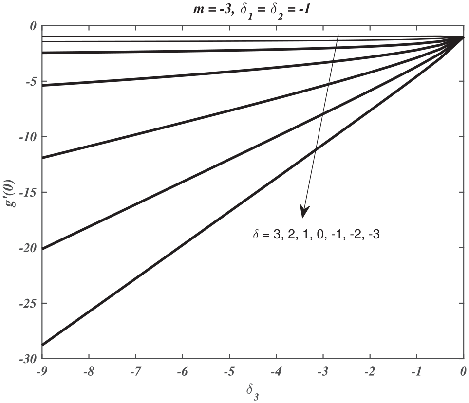
Skin fraction coefficient is plotted against

Axial velocity (normalized) is graphed against

Axial velocity (normalized) is graphed against

Axial velocity (normalized) is graphed against
In Figure 10, two sets of profiles are presented for the normal velocity component. One set of profiles is the reflection of the other about the similarity line
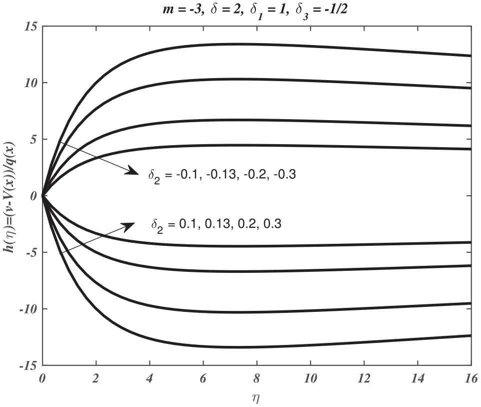
Normal velocity (normalized and translated) is graphed against
Conclusion
In this article, we have studied the flow of viscous fluid over a porous stretching/shrinking sheet of a variable thickness. Closed form solutions of the problem are found for specific ranges of the value of parameters. The power series solutions of the general problem are obtained with the combination of Padé approximation. This solution is in excellent agreement with the numerical solution. Furthermore, a detailed comparative study of the current model is presented, and remarkable results are retrieved that are available in literature on the topic. Following are the key findings of this research work:
Direct simulation of the governing PDEs is taken and pursued their similarity solutions. A set of transformations are defined for the velocity components and similarity variable. Note that the stream function formulation is not considered in the modeled problem. As a result, all the previous models of stream function formulation are recovered easily.
Multiple solutions of the final governing ODEs are found. The new solutions of the current problem are compared with classical simulations, and excellent agreement is found between them. The comparison is established in different tables and graphs.
Different and multiple solutions (closed form and series) of the model equations are presented and exactly matched with the numerical solution.
A new set of solutions is found, and these solutions are missing in the classical simulations. Ultimately, a set of new profiles in Figures 8–10 are presented and such solutions are not seen in the literature. It is one of the reasons that the flow behavior in these graphs is totally different.
Footnotes
Handling Editor: Ali J Chamkha
Declaration of conflicting interests
The author(s) declared no potential conflicts of interest with respect to the research, authorship, and/or publication of this article.
Funding
The author(s) received no financial support for the research, authorship, and/or publication of this article.