
Abstract
The recent work provides the numerical investigation of an unsteady viscous nanofluid flow between two porous plates under the effect of variable magnetic field and suction/injection. Navier Stokes equations are modeled to study the hydrothermal properties of four different nanoparticles copper
Introduction
The magnetohydrodynamic (MHD) fluid flow has so many applications in the field of engineering as well as geophysics and astrophysics. Likewise, MHD fluid flow between porous plates is applicable in designing cooling systems with liquid metals in petroleum and mineral industries, purification of crude oil, and controlling boundary layer flows. The magnetohydrodynamic fluid flow has the temperament, based on magnetic field, to overcome vorticity. Due to these innumerous applications of MHD fluid flow, a number of researchers studied incompressible fluid with and without an external magnetic field.1,2 Under the influence of a uniform transverse magnetic field, Katagiri 3 studied an unsteady hydromagnetic Couette viscous fluid, when the fluid flow within the channel is induced by the impulsive moment of one of the plates. Extending the idea of Katagiri, 3 Muhuri 4 considered the Couette viscous fluid flow within a porous channel when the fluid induced uniformly accelerated motion of one of the plates.
The study of the electromagnetic field in the fluids has gained its importance in last two decades due to its applications in nuclear fusion, chemical engineering, medicine, and transformer cooling. Ferrofluid or magnetic nanofluid is obtained when magnetic colloidal, with size range of 5–15 nm in diameter, is dissolved in a base liquid coated with surfactant layer. Sheikholeslami and Ganji 5 studied ferrofluid flow and heat transfer. They concluded that magnetic number has a strong effect on the Nusselt number as compared with Rayleigh number. Jue 6 investigated magnetic gradient and thermal buoyancy–induced cavity ferrofluid flow using semi-implicit finite element method. They identified that strengthening magnetic field results in enhancement in fluid flow.
In order to maintain a stable magnetic nanofluid, surfactants are added in the fluid which has so many applications, 7 for instance, lubrication, 8 sealing, 9 ink jet printers, 10 dampers, 11 optical filters, 12 optical sensor, 13 and cooling devices. 14 An external magnetic field is applied to make sure the attraction of magnetic nanofluids, and this phenomenon can be used in micro-electromechanical systems (MEMSs). Besides these MEMS systems, microfluidic fluids are used for heat transfer purposes. Pal et al. 15 used an external magnetic field to transport magnetic nanofluid through small channels. Moreover, an external magnetic field is also used to adjust the thermophysical properties of nanoparticles. So, it is very essential to analyze the thermophysical properties such as thermal conductivity of the magnetic nanofluids with and without the external magnetic field.
Kronkalns
16
and Elmars et al.
17
were the pioneers to study the thermal conductivity of the magnetic nanofluids with magnetite dissolved in kerosene. Although they found that there is no alteration occurred in thermal conductivity by the application of magnetic field. Doganay et al.
18
studied the thermal conductivity of the nanofluid
The convection process has many applications for industrial purposes, engineering, and in daily life uses, such as circular motion of water, when the pot of water kept on heated substance, in radiator, hot air balloon, oceanic circulation, and the stack effect. The laminar mixed convection flow with symmetric and asymmetric walls in a vertical channel is studied by Chamkha and colleagues.23,24 Umavathi et al. 25 made the numerical investigation of mixed convection, with the inertial effects, in a vertical channel. The unsteady, double-diffusive convective flow in a rectangular closed filled with a uniform porous medium is considered,26–29 and its numerical solution through finite difference method is obtained. Chamkha et al. 30 explained fully developed micropolar fluid in a channel. By natural convective combined with heat and mass transfer from a permeable surface in a porous medium studied by Chamkha and Khaled. 31
Nanofluids have so many applications in engineering as well as in medical sciences, such as surgical equipment, thermal power generation, computer storage devices, and electric and electronic appliances. Unlike the base fluid, nanofluids possess very high thermophysical properties, like thermal diffusivity, conductivity, and heat transfer ability. Due to these enriched physical properties, researchers have diverted their attention toward nanofluid dynamics.32–35 In Argonne National Laboratory (ANL), Choi was the pioneer to conceptualize nanofluid as the solvent of nanometer-sized particles in the base fluid. 36 Nanofluids are responsible to change certain base fluid properties, for instance, nanofluids occupy a relatively large surface area as compared with base fluid, which results in the reduction of kinematic energy. Due to this large surface area, nanofluids are regarded as more stable than the base fluid. Azimi and Azimi 37 modeled and simulated the GO nanofluid in a semi porous channel and verified that nanofluid is more stable than the base fluid. In the recent future, the use of nanomaterial would be an emerging field of civil engineering. Certain types of nanomaterials are widely used to enhance the mechanical properties of cementitious materials. Zhu et al. 38 studied the hydration characteristics and strength development of cement using nano-SnO2 powders with 0%, 0.08%, and 0.20% dosage. They concluded that cement strength could be greatly improved when nano-SnO2 is used with 0.08% dosage. Jawad et al. 39 discussed the three-dimensional Darcy–Forchheimer magnetohydrodynamic thin-film nanofluid containing flow over an inclined rotating plane and observed that radiation process can take place due to energy consumption. Nanofluid has also so many applications in engineering as well as in biomechanics. Prakash et al. 40 analyzed the blood flow through a tapered porous channel. They pointed out that the nanofluid flow model can be applicable in smart peristaltic pump, which may be utilized in hemodialysis. The effect of second-order slip on the plane Poiseuille nanofluid was discussed by Sultan et al. 41 Hassan et al. 42 investigate the convective heat transfer flow of nanofluid in a porous medium over a wavy surface. They pointed out that that convective heat transfer is improved by nanoparticle concentration.
Navier–Stokes equations are used to model any type of fluid flow. Therefore, the researchers analyzed Navier–Stokes equations using analytic or numerical techniques. More than all advantages of analytic or closed-form solutions, numerical solutions are more realistic and reliable due to their adaptability to all most all scientific and engineering problems. The machining precision is directly influenced by nonlinear carrying performance of hydrostatic ram. Wang et al. 43 developed a dynamic model of nonlinear supporting characters for hydrostatic ram. They carried out their simulation using finite difference techniques to obtain the variation of tool tip position and evaluate the machining accuracy. The finite difference method is used by Attia and Ewis 44 for a magnetohydrodynamic flow of continuous dusty particles and non-Newtonian Darcy fluid between parallel plates.
The magneto nanofluids have so many applications in this modern age of science and technology. For instance, it is very useful in MHD power generation, petroleum reservoirs, gastric medications, cancer therapy, and sterilized devices. The natural convection of MHD flow beyond an oscillating vertical plate in a rotating system is investigated by Patel. 45 He found that the Hall current has a tendency to improve motion in all directions. Hayat et al. 46 analyzed three-dimensional MHD flow of couple stress nanofluid. They found that thermal boundary thickness can be enhanced by radiation effect. Mesoscopic method is employed for MHD nanofluid flow by Sheikholeslami et al. 47 Their findings reveal that plume diminishes with augment of Hartmann number. The homogeneous–heterogeneous reactions in boundary flow of nanofluids are addressed by Hayat et al. 48 and concluded that the homogeneous parameters have opposite behavior for concentration profile. Muhammad et al. 49 provide the MHD boundary layer flow of Maxwell nanomaterial on a non-Darcy porous medium. Oldroyd-B nanofluid in the presence of heat generation and absorption has been formulated by Hayat et al., 50 and they found that the temperature distribution has a direct relation with Biot number. Hayat et al. 51 explore the MHD three-dimensional flow of a viscous nanofluid. They observed that magnetic number elucidates similar behavior for temperature and nanoparticle concentration.
The aim of this article is to model and numerically analyze the viscous fluid flow between two porous plates for four different nanoparticles, simultaneously. For this purpose, the Navier–Stokes equations are modified by including the porosity term within momentum equation. The governing equations for fluid flow are nondimensionalized using some suitable dimensionless quantities in order to extract some physically important parameters. The dimensionless governing equations are solved numerically using Crank–Nicolson scheme. According to our knowledge, no literature is available for dealing porous plate flow by Crank–Nicolson method.
Mathematical formulation of the problem
In this article, we consider unsteady, viscous, and incompressible nanofluid flow between two parallel porous plates at y = 0 and y = h of infinite length in the x and z directions in the presence of a variable magnetic field

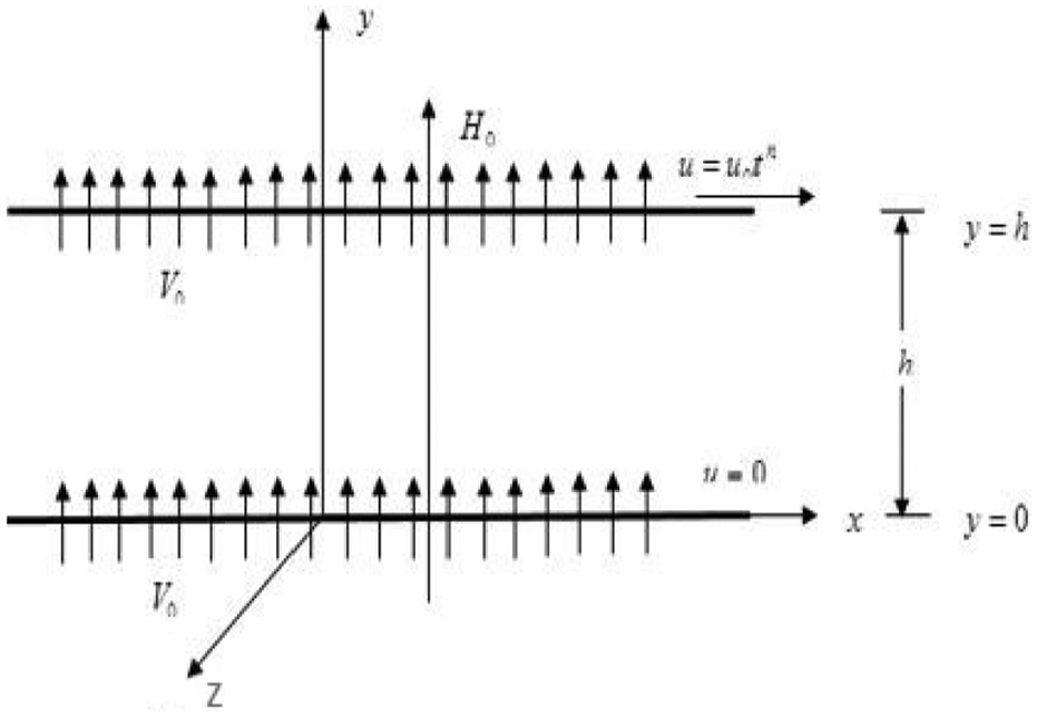
Geometry of the fluid flow.
Following the above assumptions and the proposed nanofluid model by Tiwari and Das, 53 the continuity and momentum equations take the following form: 20
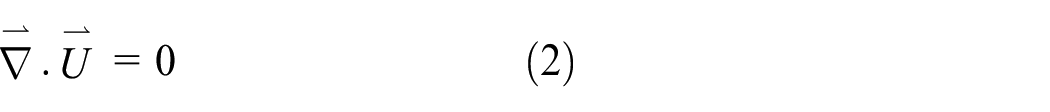
Continuity equation
Momentum equation

where

where

For a Couette flow,

After using equation (4) in the governing equation (6), we obtain
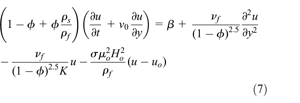
with the initial and boundary conditions

where
In order to make dimensionless the terms of the governing equation (7) along with the boundary conditions (8), and omitting * for the sake of simplicity, we use the following definitions

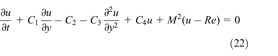
Using equation (9), the dimensionless form of equation (7) becomes

Multiplying the above governing equation by

where

Finite difference technique
The finite difference scheme is a numerical iteration method to find the solution of different terms involved in a differential equation by different quotients. It discritizes the domain in both space and time, and the solution is computed at space or at time mesh points. The modeled partial differential equation (PDE) (11) along with the boundary conditions (12) is solved by the implicit Crank–Nicolson method. Crank–Nicolson scheme replaces the velocity, and its derivative terms are given as follows


After substituting equations (13)–(16) in equation (11), we obtain the discretized form of the governing equation as

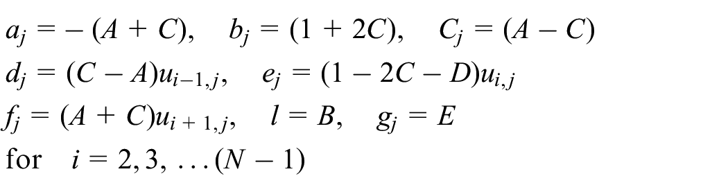
For the sake of simplicity, we suppose the following quantities

After incorporating the above quantities in equation (17), we obtain

Equation (19) represents the discrete form of the governing fluid in implicit finite different schemes. The solution of equation (19) is obtained at any space node and time level say at
Equation (19) can be represented in the tridiagonal matrix form as AU = B, where U is the unknown vector of order (N − 1) at any time matrix of order
So, equation (19) can be written as

which represents a system of linear equations in tridiagonal matrix form as

Convergence analysis of the scheme
Before discussing the convergence and stability analysis here, we state some results concerning these analysis:
Lax theorem: if a consistent linear boundary value problem is stable, then it is convergent. 55
Convergence: for linear PDEs, the fact that consistency plus stability is equivalent to converge is known as Lax equivalence theorem. 56
Note on consistency: the scheme must tend to the difference equation when steps in time and space tend to zero. A consistent scheme is one in which the truncation error tends to zero for step in time and space tends to zero. 57
In the light of the above results, we will prove that our numerical scheme is stable and convergence, for this we take our model as
The descritized form of the above equation is

Here, we defined the dependent variable as

After substituting equation (24) into equation (23) and letting

The above equation shows that the exact solution of the problem approaches to the numerical solution, so our scheme is consistent and so is convergent.
Stability analysis of the scheme
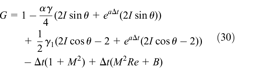
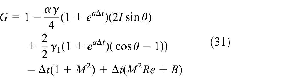
The implicit iterative Crank–Nicolson scheme has gained more importance in simulating fluid flow problems. Perhaps, two iterations are more than enough to carry out a numerical result. But the limiting case of infinitely many iterations became the well known Crank–Nicolson method. In this section, we shall explain the strategy to make sure the stability of the proposed fluid flow model. For the sake of simplicity, we consider equation (17) again without nanoproperties as below

Here,

and find the amplification factor G as, for unconditionally stable,

where

From here, we can obtain the amplification factor


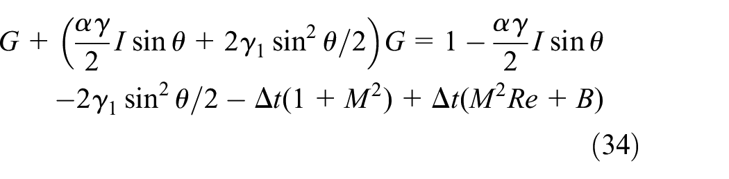

It is evident from equation (35) that the absolute value of the amplification factor
Results and discussion
The obtained numerical simulation of the proposed model is presented graphically to have an insight of the physical observation of this channel flow between two porous plates. For this purpose, the behavior of four different nanofluids is depicted through Figures 2–7 and Tables 1 and 2. The effects of some physically important parameters such as volume fraction, magnetic strength, suction/injection, and permeability parameter are examined.

Velocity for nanofluid

Velocity for nanofluid
Velocity for nanofluid
Velocity for nanofluid

3D sketch of the nanofluid flow.

Error versus parameters range for velocity profiles.
Thermo-physical properties of water and some nanoparticles. 58

Comparative effect of

Keeping in mind the thermophysical properties of nanofluid, one can use it for cooling purposes. For instance, heat capacity of a nanoparticle is the heat required to raise the temperature of the fluid. More heat is generated with increase in nanofluid volume fraction
The influence of a magnetic force on an electrically conducting fluid creates a resistant-type force called Lorentz force, which tends to accelerate the temperature and decelerate the motion of the fluid. This result is according to the desired expectations, because the magnetic force is used as a delaying force on the mixed convection flow. Application of a magnetic field moving with the free stream has the tendency to induce a motive force which decreases fluid motion and increases the nanofluid temperature. It is evident from the structure of magnetic field
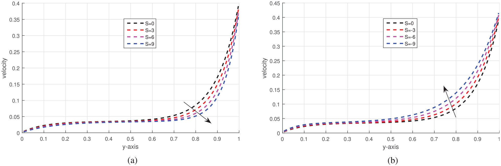
The pressure gradient is applied in the direction of fluid flow, which gives rise to the velocity profile. Figure 4(a)–(b) shows the influence of both upper and lower plate suction/injection on velocity profile. The suction effect
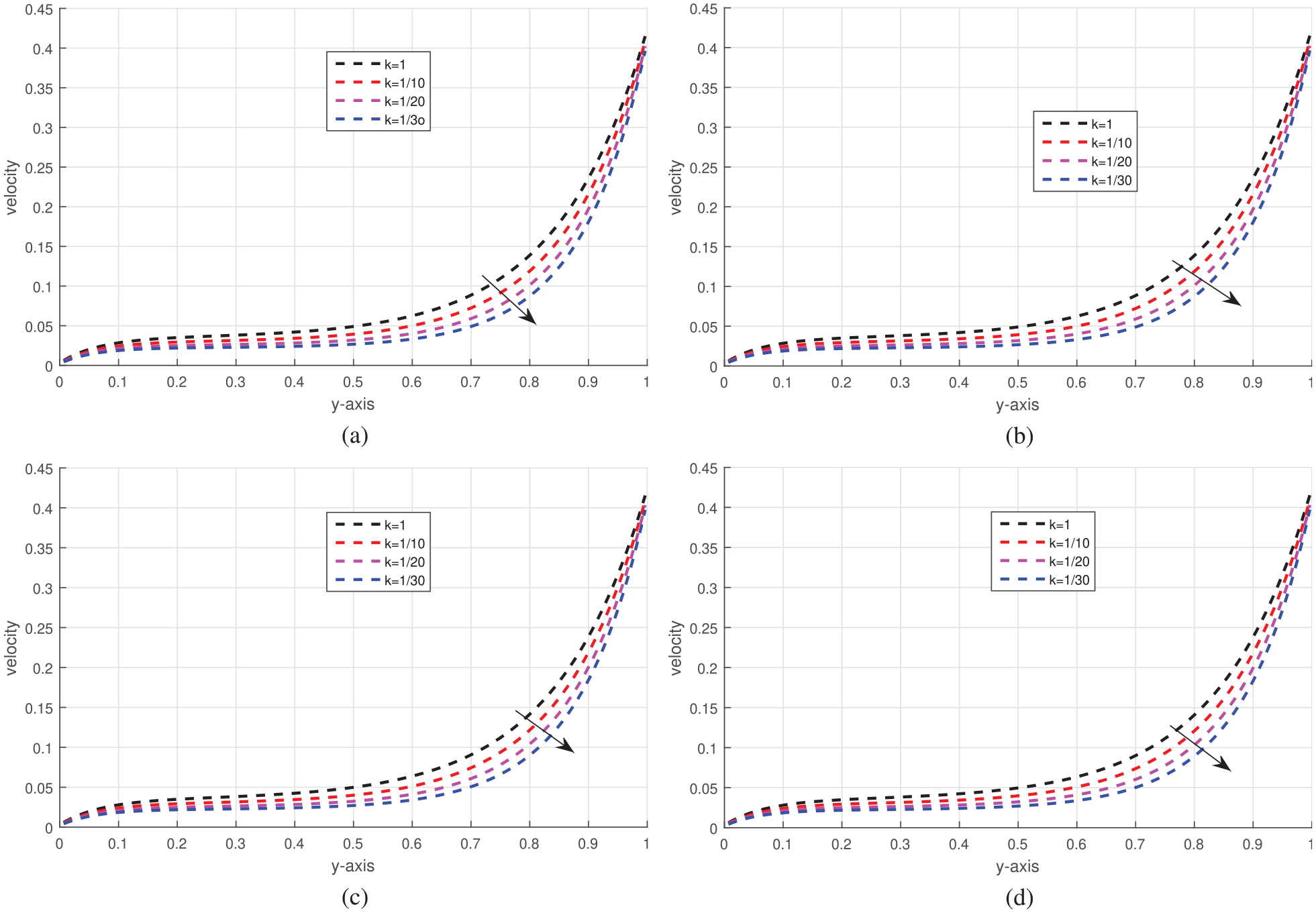
The permeability parameter
The validity of the present numerical scheme is verified by sketching the error versus parameter range graphs in Figure 7(a)–(d). The parameter’s range is selected to achieve acceptable error by Crank–Nicolson numerical method. The lower and upper bounds for the range of physical parameters are chosen in such a way that the minimum error is
It can be observed from Table 2 that on adding more nanoparticles in the nanofluids
Conclusion
The flow of four different nanofluids is discussed in more detail in this work under the effects magnetic strength and porosity parameters. For this purpose, the Navier–Stokes equations are nondimensionalized and then solved by Crank–Nicolson scheme. The present investigation enables us to conclude that nanofluids are used for cooling purposes. Moreover, the following conclusions can be drawn from this work:
A very slight variation in velocity profile occurred for nanoparticle
By lowest heat capacitance, a significant variation can be seen for nanoparticle
When the magnetic field increases, density is decreased, and as a result, the velocity of the fluid is also increasing.
The suction effect intercepts the pressure, which makes a reduction in the velocity profile.
Footnotes
Appendix 1
Handling Editor: James Baldwin
Declaration of conflicting interests
The author(s) declared no potential conflicts of interest with respect to the research, authorship, and/or publication of this article.
Funding
The author(s) received no financial support for the research, authorship, and/or publication of this article.