
Abstract
The focus of this article is to test the capability of a three-dimensional undersaturated numerical reservoir simulator developed for prediction of actual field performance cases. The simulator development employs unconditional stable Crank–Nicolson second order in time approximation discretization scheme and preconditioned conjugate gradient iterative solver for the derived fluid flow equation. Furthermore, formation volume factor as a function of cell pressure is computed at each time step until bubble-point pressure is reached. The reservoir model is then coupled with a horizontal wellbore model in the simulator by placing a well optimally at the center of its drainage volume. The numerical simulation results show that the numerical solutions improve significantly with the addition of grid blocks. Graphical visualization surface and contour map plots show rapid and continuous average reservoir pressure depletion with time for an earliest possible determination and characterization of primary drive mechanisms. The rate of pressure depletion and recovery factor estimation (1.52%) are the two main characteristics used to identify depletion drive or rock and liquid expansion drive as the best-fit prospective drive for the reservoir model. The total cumulative production of 170,000 stock-tank barrels (MSTB) recovered in 1390 days is in agreement with the field data used. Sensitivity analyses with the numerical simulator illustrated the key impact of reservoir parameters on pressure depletion with less computational expensiveness. Finally, material balance incremental (0.995) and cumulative (1.005) error checks validate the simulator robustness within an acceptable tolerance limit.
Keywords
Introduction
Primary drive mechanisms are regarded as the most important part of the early life of petroleum reservoirs’ history during modeling and simulation studies. Therefore, an earliest possible estimation is of a prime goal where an optimized accurate modeling and prediction tool is needed to forecast volumetric depletion from initial reservoir pressure, saturation pressure, and abandonment pressure. However, incorrect predictions and interpretation could skew future reservoir prudent management strategies.
Understanding the role of pressure and fluid flow in a reservoir is very keen in the development of every reservoir. However, one effective hydrocarbon recovery strategy is to take into account the effect of natural reservoir energy. 1 Several reservoir engineers have, over the past, employed strategies to understand the behavior as well as to improve the reservoir recovery factor, thus the ratio of the volume of hydrocarbons produced to the volume of original oil in place (OOIP).
Therefore, for an ultimate hydrocarbon recovery and production, understanding of the reservoir behavior and predicting future performance require knowledge of the driving mechanisms that control the behavior of fluids within the reservoirs. 2 The production of hydrocarbons from oil reservoirs by natural drive mechanism without using any other process such as fluid injection to supplement the natural energy of the reservoir is known as primary recovery.3,4 Primary recovery from hydrocarbon reservoirs is influenced by reservoir rock and fluid properties and geological heterogeneities. It is important to note that the overall performance of hydrocarbon reservoirs is largely determined by the nature of the energy, that is, driving mechanism, available for moving the oil and gas to the wellbore. To add to the above, the natural reservoir energy controls the ultimate recovery of hydrocarbons during primary production. 5 An oil reservoir is said to be undersaturated if the reservoir pressure (Pi) is higher than the bubble-point pressure (Pb) (Pi > Pb) and has a small constant compressibility. 6 Nevertheless, at pressures above the bubble-point pressure, crude oil, connate water, and rock are the only materials present with a constant gas–oil ratio (GOR) that is equal to the gas solubility at the bubble-point pressure. 7
Basically, six primary drive mechanisms exist. These six primary drive mechanisms provide the natural energy necessary for oil recovery. Rock and liquid expansion drive, solution gas drive (depletion drive), gas-cap drive, natural water influx (water drive), gravity drive, and combination drive processes are the six primary drive mechanisms. Depletion drive reservoir can be known by the pressure behavior and the continuous and rapid decline of reservoir pressure. This reservoir pressure behavior is attributed to the fact that no extraneous fluids or gas caps are available to provide a replacement of the gas and oil withdrawals.
In addition, the absence of a water drive means there is a probability of little or no water production with the oil during the entire producing life of the reservoir. A depletion drive reservoir is characterized by a rapidly increasing GOR from all wells, regardless of their structural position. After the reservoir pressure has been reduced below the bubble-point pressure, gas evolves from solution throughout the reservoir. Once the gas saturation exceeds the critical gas saturation, free gas begins to flow toward the wellbore and the GOR increases. The gas then begins a vertical movement due to gravitational forces resulting in the formation of a secondary gas Oil production by primary drive can be agreed as an efficient recovery method. 8 This is a direct result of natural energy throughout the formation of the reservoir. Primary recovery from undersaturated oil reservoirs depend on rock and fluid properties as well as heterogeneities leading to an average recovery factor of 34% with the remaining oil in place left unproduced in the reservoir. 9 The recovery from these types of primary drive reservoirs suggests that quantities of oil are remained in the reservoir when the reservoir pressure reduces, therefore the need to predict primary drive mechanistic behavior as well as to maximize reservoir performance. In order to have a better understanding of the reservoir behavior, the nature of energy, and forecast of the future performance, it is essential to have good knowledge of primary drive mechanisms that would be suitable to control fluid flow in porous media for an eventual oil and gas field development technique. 10 This is the major reason why this current article embraces depletion drive mechanism as a standard for comparing other producing typical drive mechanisms for reservoir performance to serve as the first valuable knowledge of improving reservoir performance and maintaining the best reservoir management. 11
Schilthuis 12 introduced material balance technique to provide insights into reservoir drive mechanisms, the production characteristics of the reservoir, and the determination of initial oil in place under different types of primary drive mechanisms. This method is also used for calculating the decline in average reservoir pressure depletion. The Schilthuis material balance equation has long been regarded as one of the basic tools for reservoir engineers for interpreting and predicting reservoir performance. The application of material balance has been acknowledged by several researchers for analyzing petroleum reservoirs with simplifying assumptions especially in the works of Yang et al. 13 , Xu et al. 14 , and Habibi et al. 15 Adeloye et al. 16 described material balance as zero-dimensional simulator since there are no changes in any direction within the reservoir system being seen as a serious drawback. Buduka et al. 17 in their work also used graphical material balance as an equation of a straight line to estimate reservoir fluids in place but with some drawbacks. The material balance equation possesses high degree of inaccuracies of the measured reservoir pressure, and the model fails when decrease in reservoir pressure is not feasible, such as in pressure-maintenance operation. 18 Adeloye et al. 16 presented the material balance equation for undersaturated reservoirs. In their work, they tried to resolve these difficulties by developing a statistical material balance simulator that would predict initial oil-in-place and reservoir properties under water drive. Their work defined the properties of reservoir fluid using pressure volume temperature (PVT) models as well as evaluating the volume of water influx into the reservoir from the aquifer using Van Everdingen and Hurst aquifer model. A development of an inverse statistical method to estimate stock-tank initial oil-in-place and reservoir properties from material balance can be seen in their work. 16 Although the classical material balance techniques are still in use, they have now been largely superseded by numerical simulators, which are essentially multi-dimensional and multi-phase dynamic material balance programs. The classical approach is well worth studying since it provides a valuable insight into the behavior of hydrocarbon reservoirs. 19 Sureshjani et al. 20 used material balance to do early estimation of the size of newly discovered expansion type of reservoirs. However, their work observed a sizable decline in pressure drop incident in the production of oil above bubble-point pressure. In addition, their research also presented a further extension of the material balance equation applied to volumetric undersaturated reservoirs above the bubble point by including a term for interstitial water compressibility. Material balance analysis of reservoirs as tank models leads to the development of large reservoir models using grid blocks to provide a valuable insight into the behavior of hydrocarbon reservoirs. The principal assumptions of several inaccurate calculation and prediction of oil recovery and actual field performance has resulted in the use of numerical methods. Simulation and modeling of petroleum reservoir performance refers to the construction and operation of a model whose behavior depicts the appearance of an actual reservoir behavior. Hashan et al. 21 explained reservoir simulation as an engineering tool that gives insight into the dynamic reservoir and fluid properties behavior of reserve estimation and evaluation of past and future reservoir performance. Jha et al. 22 described reservoir simulation and modeling as the science of combining physics, mathematics, reservoir engineering, and computer programming to develop a tool for predicting hydrocarbon reservoir performance under various operating strategies. Ertekin et al. 23 stated that reservoir simulation and modeling might be the only reliable method to predict performance of large complex reservoirs. This assertion was supported by Johnston et al. 24 that a reservoir simulation and modeling when combined with three-dimensional (3D) time-lapse seismic results can be used to monitor past and future production performance. The major goal of reservoir simulation is to predict future performances of reservoirs and find ways and means of optimizing the recovery of hydrocarbons under various operating conditions.
Efforts on reservoir modeling as well as the understanding of flow characteristics in unsteady-state gas flow in homogeneous reservoirs have also been made continuously. 25 Among the commonly used conceptual models is the implicit numerical simulator for depleted-drive reservoirs. This implicit numerical simulator designed for depleted-drive reservoirs is widely used in petroleum engineering because of its ability to match many types of laboratory and field data notwithstanding its utilization in commercial software. 8 Some numerical simulations 26 and analytical solutions have been proposed for oil flow in unsteady-state gas flow in homogeneous reservoirs. However, analytical solutions can only be obtained under much idealized assumptions, such that slight compressibility, infinite radial flow, homogenization, and many more found in their applications are restricted to simplified cases of oil flow. For gas flow, slight compressibility assumption is not held any more. The governing equations are nonlinear and cannot be analytically solved.
Numerical computations for undersaturation in homogeneous reservoirs often pose some difficulties. Therefore, it is important to study numerical methods for depletion of unsteady-state gas flow in homogeneous reservoirs based on an implicit numerical simulation. Owusu et al. 27 developed a Muskats model to analyze solution-gas drive reservoir to predict its primary oil recovery. The inflow and outflow performance of the reservoir was analyzed and the future performance of reservoir was also forecasted. Bruce 28 was the first author to use numerical method for calculating pressure distributions for unsteady-state gas flow in homogeneous reservoirs. The general acceptance since then can be attributed to advances in computing resources and numerical techniques for solving nonlinear partial differential equations (PDEs) that cannot be solved analytically. 19
An implicit numerical simulator for expansion-drive reservoirs was developed by literature.19,20,29,30 The contribution of their work is limited to increase the size of grid blocks developed by the simulator, thereby resulting in numerical solution convergence problems and high computational cost. Lie et al. 31 and Stein et al. 32 proposed a toolkit implementation for discretization and solution methods for subsurface flow simulation on general and complex grids. However, the two-point flux approximation methods employed were only consistent for K-orthogonal grids but eventually suffered a convergence problem with grid-orientation effects.
Aphu et al. 33 developed one-dimensional (1D) finite difference explicit and implicit numerical reservoir simulator for modeling single-phase flow in porous media. The explicit and implicit simulator developed in their study consisted of physical modeling, mathematical modeling, discretization of the models with finite difference scheme, and transformation of the models into computer algorithms. The explicit and implicit simulators showed that the implicit formulation is unconditionally stable than the explicit formulation. A two-dimensional implicit numerical simulator for expansion-drive reservoirs was developed by Omosebi. 34 However, their numerical studies show a rapid pressure decline for an expansion-drive reservoir due to insignificant compressibility that typifies rock and fluid properties. It was revealed that no 3D character of real reservoirs was accounted for in their work. The study Dele et al. 35 accounted for the Z-direction of flow by developing a 3D reservoir simulator for expansion-drive reservoirs, but their work was limited to implicit formulation which did not employ preconditioned iterative solvers for fast solution convergence. In order to develop these reservoir models, Cheng-yong Li et al. 36 illustrated in their work the simulation and modeling procedure to be adopted. First, the development of a physical model with relevant recovery process and the essential features of the underlying physical phenomena were characterized. Second, a set of coupled systems of temporal and spatial dependent nonlinear PDEs was developed and analyzed for existence, uniqueness, stability, and regularity. Third, a numerical model with the basic properties of both the physical and mathematical models was then obtained and analyzed. Fourth, computer algorithms (programming codes) were developed to solve efficiently the systems of linear and nonlinear algebraic equations arising from the numerical discretization.
Based on the aforementioned development, the current research uses Crank–Nicolson formulation over the implicit formulation for accurate and reliable numerical solution at larger time steps and at no extra computational cost. In numerical analysis, the Crank–Nicolson method is a finite difference method used for numerically solving the heat equation and similar PDEs. A 3D numerical simulator is developed by using unconditional stable Crank–Nicolson scheme and preconditioned (used to reduce the matrix condition number and speed up the convergence of the iterative solver in order to increase the convergence rate) conjugate gradient iterative solver for initial possible determination of the degree of initial undersaturation and recovery of primary drive mechanisms. A reliable and accurate initial estimation until bubble-point pressure is reached provides the possibilities of enhancing primary recovery.
Hence, this article aims at developing a robust 3D undersaturated oil numerical reservoir simulator with graphical user interface (GUI) to model and predict reservoir parameters through time to optimize recovery efficiency under primary drive reservoirs.
In addition, this research also presents systematic mathematical data structures and programming algorithms to describe and characterize primary drive reservoirs on structured grids. The numerical reservoir simulator reliability and robustness used in this current research are validated with material balance method for full-field reservoir simulation studies.
This research work is organized into four sections as follows: “Introduction” section gives introduction of primary drive recovery and unconditional stable Crank–Nicolson scheme preconditioned for possibilities of enhancing primary recovery from the literature. “Methodology” section describes the physical formulation model, the mathematical model, mathematical fluid flow equations, numerical modeling, computer modeling for Crank–Nicolson formulation, and horizontal wellbore modeling in the simulator by placing a well optimally at the center of its drainage volume. “Results and discussion” section discusses key results obtained from the numerical simulation and oil recovery factor and performance. Finally, “Formation volume factor (FVF) analysis” section summarizes the conclusions drawn from this study for future integration into reservoir models with Crank–Nicolson formulation method.
Methodology
Physical model formulation
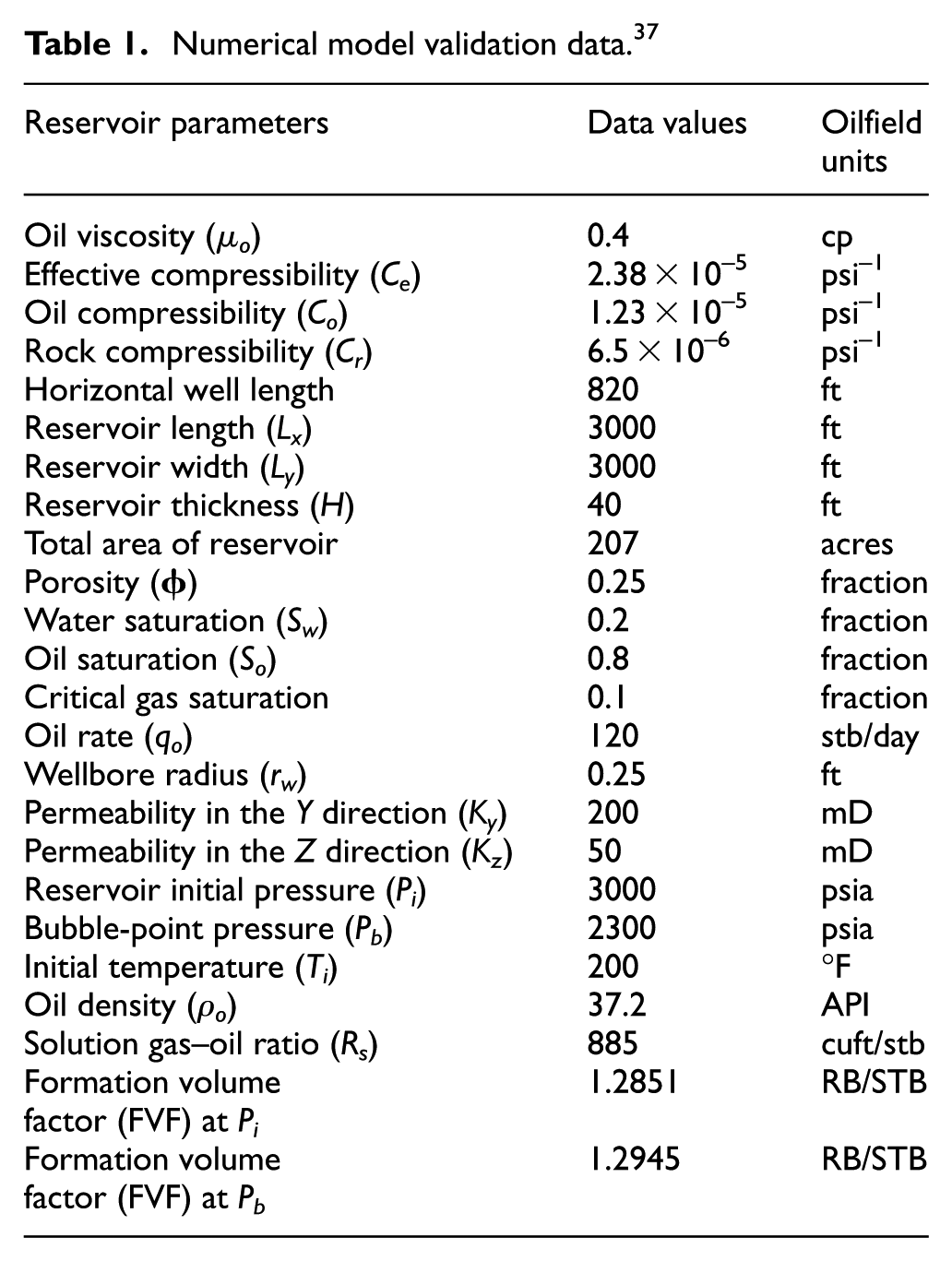
This study uses rock and fluid properties data given in Table 1 37 to populate a 3D reservoir model represented by regular grid blocks as shown in Figure 1. A horizontal well is drilled at the center of the reservoir model to drain the hydrocarbons underground. The model has grid dimensions of 11 × 11 × 11 cell size (base case) with no flow boundary condition implemented. 38 In addition, 15 × 15 × 15 grid dimensions were also tested in this study. The reservoir is initially filled with oil and irreducible water saturation in hydrodynamic equilibrium. The initial reservoir block pressure is specified before advancement of the pressure solution in time. The pressure distribution in a slightly incompressible flow problem changes with time and is solved in unsteady-state form. The derived fluid flow equation is written for every discretized reservoir block by solving the resulting set of linear equations for the set of unknown pressures. The initial time and time step change are specified for finding pressures at discrete times until desired simulation time is reached.
Numerical model validation data. 37

Schematic view of three-dimensional (11 × 11 × 11) discretized reservoir grid system.
Mathematical modeling
The reservoir characteristics are normally expressed in terms of a set of coupled PDEs together with the appropriate initial and boundary conditions that approximate the behavior of the reservoir. The three main laws governing isothermal reservoir simulation employed in this current research are as follows:
The law of mass conservation;
Darcy’s law (transport equation);
Equation of state (compressibility and FVF).
Mathematical model basic assumptions
The mathematical model is developed with the following basic underlying assumptions:
Isothermal, homogeneous, and anisotropic reservoir;
Fluid and rock properties are slightly compressible;
Uniform grid size with block-centered Cartesian coordinate system;
No-flow reservoir boundary condition (water influx is negligible);
Constant compressibility and GOR above bubble-point pressure;
The fluids are Newtonian; capillary and gravity forces are ignored;
Chemical reactions are not included.
Mathematical fluid flow equation
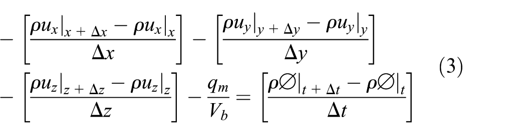
Applying the law of mass conservation for isothermal reservoir simulation for single-phase flow can be represented in equations (1)–(4) as


Taking limit as

where
Second, applying a constitutive equation of Darcy’s law that relates the volumetric flow rate to fluid potential in equation (5) is expressed as

where
Third, applying slightly compressible fluid flow equation expressed in equation (6) is written as
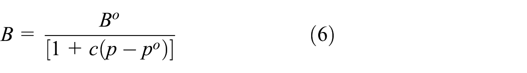
where B is the FVF, Bo is the FVF at reference pressure, c is the fluid compressibility, p is the reservoir pressure, and po is the reference pressure.
The final form of equation after simplifying and applying the three laws governing isothermal reservoir simulation is given in equation (7) as
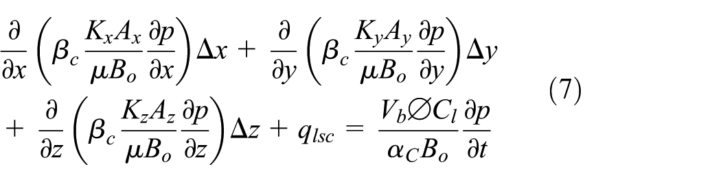
where
The initial conditions for undersaturated oil reservoir at single-phase equilibrium is given as
The boundary conditions are specified pressure gradient boundaries for the closed unit reservoir seen in Figure 1, which are expressed as:
Numerical modeling
Crank–Nicolson 39 1947 method is a finite difference method used to numerically solve PDEs. It involves combination of old and new time step values of the dependent variable. It is a second-order approximation in time and numerically stable than implicit formulation. The advantage of the Crank–Nicolson formulation over the implicit formulation is a more accurate solution for the same time step or larger time steps. 40 This gain in accuracy is obtained at no extra computational cost. The drawback of the Crank–Nicolson formulation is that the numerical solution may exhibit overshoot and oscillations for some problems. Such oscillations are not due to instability but rather an inherent feature of the Crank–Nicolson formulation. 40 However, such artificial oscillations can be minimized by using total variation diminishing schemes.41,42 Studies on linear and nonlinear differential equations have been implemented to model various problems in a number of fields. 43
The three-dimensional mathematical model derived in equation (7) is too complex and intractable by an analytical method. Therefore, Crank–Nicolson finite difference approximation scheme is used to truncate the derived equation into a form that is amenable to numerical solution by digital computer. This discretization process involves applying spatial (central differencing scheme approximation) to left hand side of equation (7) and time (backward difference approximation) to right hand side of equation (7) as shown in equations (8) and (9)

Simplifying and rearranging like terms

where
Mathematical relations implemented in the computer model
The following mathematical relations were implemented in the numerical simulator developed in MATLAB programming environment.
The FVF for the mathematical model derived is calculated in equation (10) as

The cumulative production, Np, is calculated in equation (11) as

where

The cumulative production from the entire reservoir, Ntp, grid block is calculated in equation (12) as

Production rate q from each grid block at each time step of simulation is calculated in equation (13) as

Average reservoir cell pressure (paverage) is therefore calculated in equation (14) as

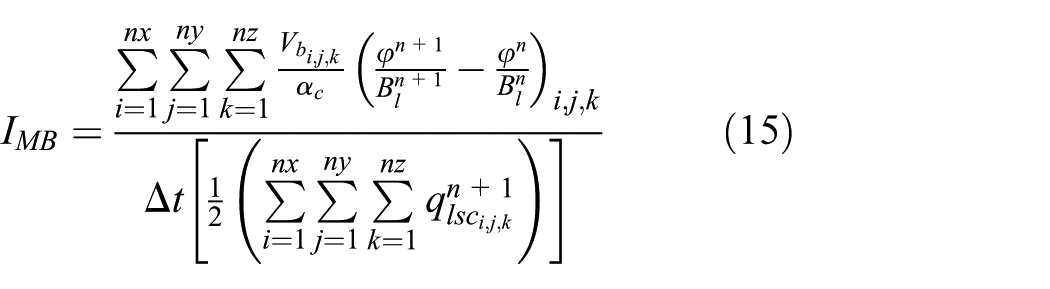
The material balance error check performed over a time step is known as the incremental material balance check, IMB, and is expressed in equation (15) (Ertekin et al.) 23 as
The material balance error check performed from initial reservoir conditions to entire time period of simulation is known as the cumulative material balance check which is expressed in equation (16) (Ertekin et al.) 23 as

where
Therefore, the average compressibility of the undersaturated oil between initial and bubble-point pressure is presented in equation (17) as

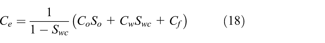
Effective or saturated-weighted compressibility of the reservoir system is given in equation (18) as
The recovery factor is calculated using the equation (19) as

Computer modeling for Crank–Nicolson formulation
The numerical model obtained for the three-dimensional single-phase flow oil reservoir using Crank–Nicolson formulation equation requires high-speed digital computer for implementation due to the large band of matrix generated. In this research, a computer program is written in MATLAB programming environment 44 for the numerical model with steps shown in Figure 14 (Appendix 1). The steps and equations used in the development of the computer codes are as follows:
A GUI that accepts input data (rock, fluids, wells location, and production rate) is designed as shown in Figure 2.
The computer program calculates the interblock transmissibilities coefficient from the initial reservoir parameters entered in the GUI interface for all reservoir grid blocks.
The unknown pressures are placed at the left hand side of the fluid flow equations for each grid block (at the time level n + 1) while the known quantities are placed on the right hand side of the equations.
The computer program generates a system of linear algebraic equations to be tractable by an iterative solver after applying reservoir initial and boundary conditions.
The computer program solves the resulting set of linear algebraic equations for the set of unknown pressures (at the time level n + 1) using preconditioned conjugate gradient iterative linear equation solver until convergence criterion is satisfied.
The computer program advances pressure solution in time with new time-level estimates serving as known estimates for subsequent iteration until the desire end of simulation time is reached.
The computer program performs incremental and cumulative material balance error checks to validate the performance of the simulator developed within acceptable tolerance limit.
The program output simulation plots are made at the end of each time step of the computations with contour and surface plots of the average reservoir pressures as well as cumulative production, FVF, and production rates versus time.
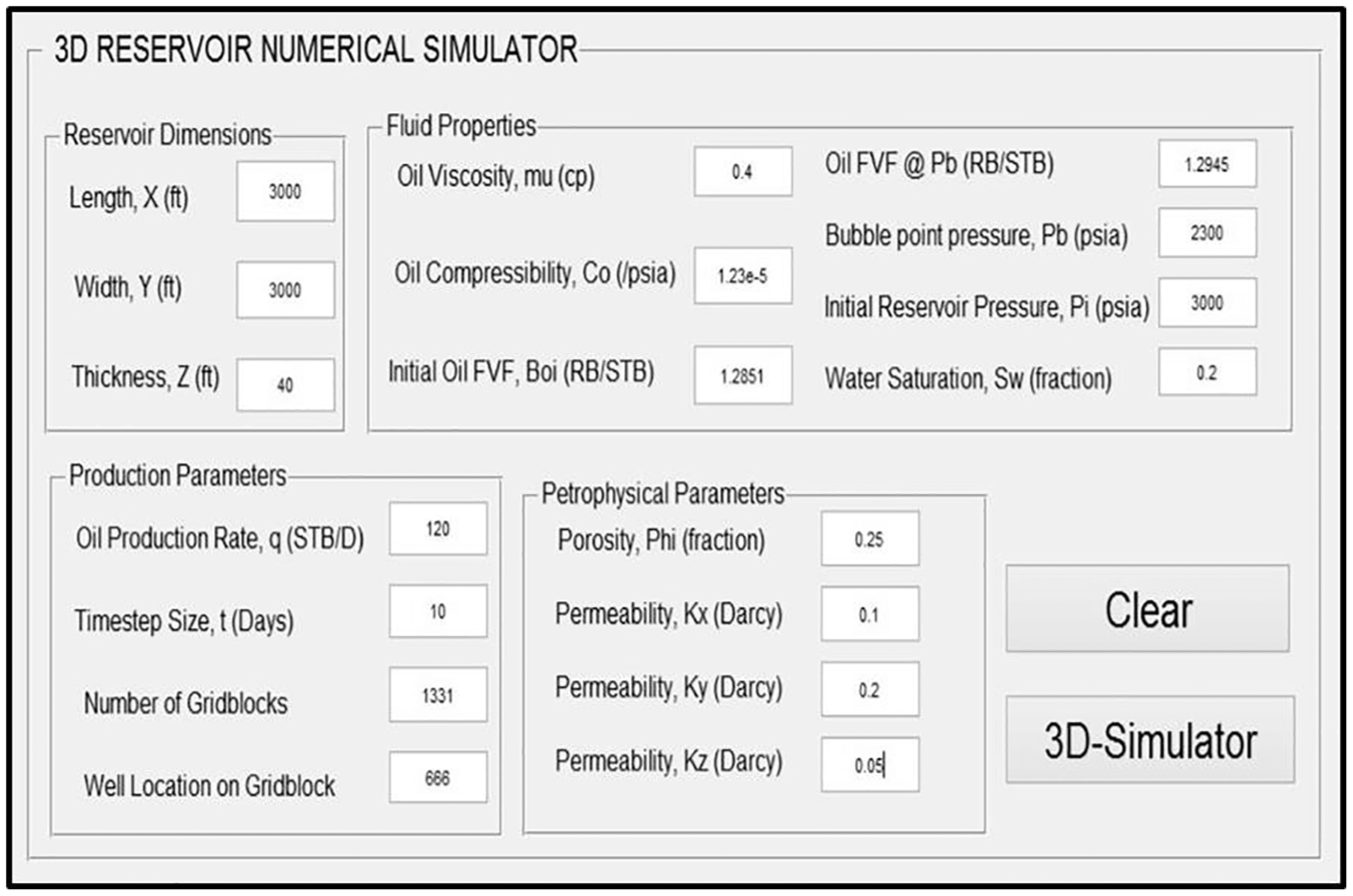
Three-dimensional numerical simulator graphical user interface (GUI).
Horizontal wellbore modeling
One of the ultimate goals of the study of reservoir modeling and simulation is to forecast hydrocarbon reservoir well flow rates and bottom hole flowing pressures accurately to maximize productivity index. Recently, attention has been drawn to horizontal wells in petroleum literature. This is due to the fact that horizontal wells have larger contact area and can be oriented to high permeability channels than vertical wells in draining equivalent reservoir volumes and also minimize coning problems. The disadvantages are that only one pay zone can be drained per horizontal well, not to mention the cost involved. 45 Wells are considered to be internal boundaries of system; there are two types of internal boundary conditions which can be specified for wells called the sandface pressure specification (Dirichlet type boundary condition) and flow rate specification (Neumann type boundary condition). 6 In this study, Neumann type of boundary condition is specified for the horizontal wellbore modeling. Well treatment in reservoir simulators comes with some difficulty which requires special considerations. 23 One logical approach to reduce the complexity of the solution is to use Peaceman vertical well model (on the assumption that the grid spacing and permeability are uniform, the well is isolated (not located near any other well), and the well is not near any other grid boundary) by rotating the axes of the model to account for the horizontal well. In this modification, the lines y and z axes are interchanged if the horizontal well is placed parallel to the y direction, so that the equation is expressed in equation (20),23,46 implemented with no wellbore damage, as
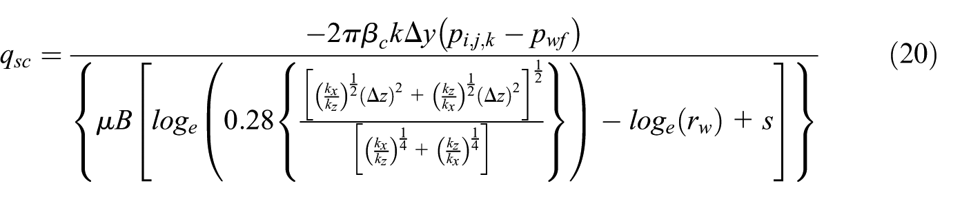
Note that if the horizontal well is placed parallel to the y direction, the y and z axes are interchanged and the k in the numerator, therefore, becomes 23

where rw is the wellbore radius, pwf is the bottom hole flowing pressure, and s is the skin factor.
Peaceman horizontal well productivity equation is now given by equation (21) as
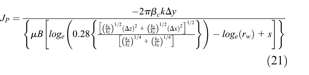
where
Results and discussion
Application of simulator to oilfield problem (field example)
The undersaturated numerical simulator developed is tested using West Texas black oil reservoir data obtained from literature shown in Table 1 to evaluate its performance of capturing main features that characterized undersaturated reservoirs. 37 For simplicity, the reservoir depleted is only a single horizontal well drilled at the center of the reservoir acreage.
Average reservoir pressure analysis
The plot in Figure 3 shows average reservoir pressure depleted with time for grid block size of 11 × 11 × 11 as shown in Figure 1. The spatial average pressure distribution approximations calculated at each time step are different depending on the time step size used in the computation (Δt = 10 days). However, smaller time step sizes gave more precise results when compared to larger time step sizes when specified in the numerical simulator. In addition, the pressure transient created by fluid withdrawal from the horizontal well is felt around the center of the well than the boundaries of the reservoir and can move more than one grid block per time step. 25 The OOIP for this model is 11.9 MMSTB. The three-dimensional reservoir simulator has been able to predict the average reservoir pressure decline from 3000 psia to saturation pressure of 2300 psia in 1390 days before any eventual pressure maintenance or enhanced recovery program to improve flagging production.26,47 It can be inferred from Figure 3 that the average reservoir pressure was rapid and continuous until saturation pressure is reached in 1390 days. In Dele et al. 35 with the same grid block sizes, the saturation pressure was reached in 1180 days for the implicit simulator used. Hence, the two possible drive mechanisms identified are depletion drive and rock and liquid expansion drive according to Ahmed and McKinney 48 and Satter et al. 49 using rate of pressure depletion and oil recovery efficiency. The slope (–0.5068) from Figure 4 is used to estimate the reservoir bulk volume to validate the simulator developed using equation (22) as

where
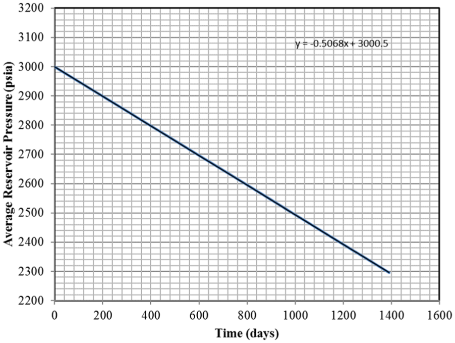
Average reservoir pressure versus time.

(a) Surface map for grid block size 11 × 11 × 11, (b) contour map for grid block size 11 × 11 × 11, (c) surface map for grid block size 15 × 15 × 15, and (d) contour map for gridblock size 15 × 15 × 15.
Using equation (26) gave reservoir bulk volume of 3.58 × 108 ft3 while the reservoir dimensions from Table 1 gave a reservoir volume of 3.60 × 108 ft3 which shows that the estimated volume from the developed simulator and volumetric estimate have good agreement.
Surface and pressure contour map plots
This section dwells on surface and contour plots of average reservoir pressure distribution at specified time before saturation pressure. The other grid dimension tested in this study is 15 × 15 × 15 for the three-dimensional model with the base case being 11 × 11 × 11. Surface and contour maps of Figure 4(a)–(d) represent the spatial rapid pressure distribution with time unlike in the works of Omosebi 34 where the behavior of the pressure shows a decline but not a rapid decline such that the decline is slow even with withdrawal, thus prolonged production life of the reservoir. The surface plots (Figure 4(a) and (c)) indicated that as grid block dimension increases, the numerical solutions improve significantly, resulting into more detailed description of the model for primary drive identification. The color scale bar also illustrated that pressure distribution is very low near where the horizontal well is drilled as compared to the reservoir boundary. The range of interest of pressure distribution map (assuming the model is sealed off to fluid flow) exists with the flux vanishing everywhere on the boundary. The contour maps drawn are two-dimensional representations of the reservoir pressure distributions. The contour lines depict the pressure distribution in the reservoir over time connecting points of equal pressure elevations in the reservoir. It also shows pressure elevation above the reference saturation pressure drawn at contour intervals. Finally, it is revealed that as grid block dimensions increases to 15 × 15 × 15, the contour lines (Figure 4(d)) become closer with greater pressure depletion unlike in Figure 4(b).
Cumulative production analysis
Figure 5 shows a plot of total cumulative production from each grid block versus time. This indicates the amount of oil that can be recovered from the reservoir model until saturation pressure is reached. The total amount of oil recovered using the developed simulator is 170 MSTB in 1390 days. Therefore, in this research study, the cumulative production from material balance for undersaturated reservoir using equation (23) gave a result of 180 MSTB which has a good agreement with the simulator developed (Figure 5). The slight difference might be due to rounding off because of computers’ finite word length 34

where

Cumulative production versus time.
Oil production rate analysis
The plot seen in Figure 6 depicts oil production rate from the horizontal well drilled in the reservoir with a constant production rate of 120 stb/day. However, from the simulation results, it can be inferred that during the first and second time step, unsteady-state (transient) flow 11 occurs before flow rate is stabilized. This constant production rate is maintained throughout the production period of 1390 days. Mathematical calculation using equation (24) gave a production rate of 199.99 stb/day which has a good agreement with the initial rate specified (Neumann type of internal boundary condition for horizontal wellbore).

Authors like Dele et al. 35 with their implicit simulator had a similar result of 200 stb/day of the oil recovered in 1180 days of production which is similar to Figure 6 in this study.

Oil production rate versus time.
Ultimate oil recovery factor analysis
The recovery factor at any time step can be calculated from initial reservoir conditions until saturation pressure is reached using equation (25)5,11

The estimated recovery factor at saturation pressure is 1.52% of OOIP. The pressure difference from initial reservoir pressure to saturation pressure is 700 psia which resulted in this low recovery factor estimated at saturation pressure. Glover 5 and Ahmed 3 described this type of primary drive as depletion or rock and liquid expansion-drive mechanism and further explained the least efficient recovery mechanism above saturation pressure. However, above saturation pressure, GOR remains constant due to dilution; hence, further distinction in the best-fit prospective primary drive reservoir can only be made after critical gas saturation is exceeded for this model. In addition, for depletion drive, GOR increases to a maximum and declines, while for rock and liquid expansion drive, GOR virtually remains low and constant.47–49 Figure 7 represents rapid pressure decline with calculated recovery factors above saturation pressure for natural drive mechanisms. The recovery factor computation at various pressures above saturation pressure determines prospective drive mechanism to be depletion drive or expansion type. The predictions made here should be in good agreement with a field performance value when plotted on the same graph. 27

Average reservoir pressure versus recovery factor.
FVF analysis
FVF is a function of pressure used to change the volume of oil at reservoir pressure and temperature to its equivalent volume at standard conditions.50,51 The FVF implemented in the simulator developed in this research is not kept constant, but calculated at each time step until saturation pressure is reached using equation (8). Figure 8 illustrates the oil FVF versus average reservoir pressure. It can be inferred from Figure 8 that FVF in the undersaturated region increases as pressure decreases due to expansion of oil and its solution gas. Nevertheless, as average reservoir pressure decreases in the saturated region, oil phase shrinks because of gas coming out of solution resulting into decrement of FVF with gas evolution dominating oil expansion due to pressure depletion.

Oil formation volume factor versus average reservoir pressure.
Sensitivity impact of key parameters on reservoir performance
Sensitivity analysis is an important part of any reservoir modeling and simulation studies which help to generate many realizations on the reservoir before making any reservoir management decision. This process is done by altering some key reservoir parameters of the model repeatedly to run and observe the net effects of the varied parameters with an acceptable level of accuracy. Sensitivity analysis results from the simulator were used to generate plots to have better visualization of the simulation and interpretation of reservoir key parameters on primary drive reservoirs. The parameters considered in the sensitivity analysis of this research include water saturation, porosity, effective compressibility, reservoir thickness, cumulative production, and production rate.
Sensitivity impact of water saturation on average reservoir pressure
In undersaturated reservoirs, the pore space in the reservoir system is occupied by oil and connate water for the model under study for reserve estimation. 52 It can be seen from Figure 9 that as average reservoir pressure depletes with time, connate water from the base case of 20% increased to 40% and 50%. This can potentially lead to early water encroachment as a result of the connate water expansion. Omosebi and Igbokoyi 29 explained that the fraction of water in place in the reservoir affects simulation results. However, their findings show that increase in water saturation results in sharp pressure decline as well as the time to arrive at bubble point is significantly shortened by increasing water saturation. In this article, it is also observed from the plot that it takes less time for 50% connate water saturation to reach saturation pressure than 20% and 40% connate water saturation. It can also be seen that a reduction in reservoir pore volume can also have an impact on connate water saturation as well as the bulk volume of the reservoir indicated in equation (26) as


Sensitivity impact of water saturation on average reservoir pressure (Sw = 0.2, Sw = 0.4, and Sw = 0.5).
Sensitivity impact of porosity on average reservoir pressure
In a single-phase slightly compressible flow problem, porosity of the reservoir formation is a function of average reservoir pressure according to equation (27)

Sensitivity analysis of porosity is varied from the base case of 25% to 10% and 40% as illustrated in Figure 10. It was revealed from the plot that for 10% porosity value, the average reservoir pressure decreases drastically, but takes less time for saturation pressure to be reached. While for a porosity of 40%, although a time decrease is expected, it takes a longer time for saturation pressure to be reached. However, Figure 10 confirms similar result was obtained by Aphu et al. 33 for the sensitivity analysis performed to investigate the effect of porosity on average reservoir pressure. Average reservoir pressure declined as the porosity decreases from 30% to 10% indicating that the time taken to reach the bubble-point pressure also decreases as the porosity decreases.
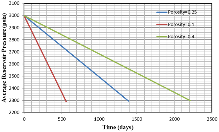
Sensitivity impact of porosity on average reservoir pressure.
Sensitivity impact of effective compressibility on average reservoir pressure
Figure 11 visually illustrates the change in pore volume per unit change in pressure depletion for rock and fluid expansion in the model. This is estimated from equation (28) as

As effective compressibility is decreased from the base case of 2.38 × 10⁻⁵ psi–1 to 1.2 × 10⁻⁵ psi–1, the rate of average pressure decline increases rapidly and the time taken to reach saturation pressure is fast. However, for compressibility of 3.42 × 10⁻⁵ psi–1 above the base case, the time taken to reach saturation pressure is prolonged. This behavior is in agreement with similar study reported by Onolemhemhen 1 and Appiah. 30
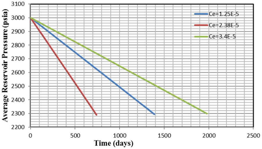
Sensitivity impact of compressibility on average reservoir pressure.
Impact of net pay thickness on average reservoir pressure
The reservoir net pay thickness is a vital reservoir parameter used in estimating the OOIP of a reservoir.53–55 The net pay thickness helps evaluate the section of the reservoir where the horizontal well is drilled for production optimization in this study. Figure 12 shows a plot of average reservoir pressure versus time when reservoir thickness is varied from the base case. It can be inferred from the graph shown in Figure 12 that as reservoir net pay thickness is decreased to 20 ft, less time is taken to reach saturation pressure when pressure drops. Meanwhile, increasing the thickness to 50 ft above the base case increased the time required to attain saturation pressure with similar results obtained by Dele et al. 35

Sensitivity impact of net thickness on average reservoir pressure.
Sensitivity impact of production rate on average reservoir pressure and cumulative production
Sensitivity impact of varying production rate on average reservoir pressure and cumulative production is presented in Figure 13(a) and (b). If production rate is switched to 90 stb/day from the base case of 120 stb/day, the time taken to reach saturation pressure is delayed as compared to when production rate is increased to 130 stb/day with less time. Therefore, production rate optimization is needed for 130 stb/day in order to sustain the life of the well drilled if there is no additional pressure support. Cumulative recovery from production is also influenced as a result of varying production rate. This claim is consistent and in agreement with similar findings by Omosebi and Igbokoyi 29 and Dele et al. 35 It can be seen that more oil is recovered if production rate is maintained at 90 stb/day as compared to increasing production rate to 130 stb/day in Figure 13(b).
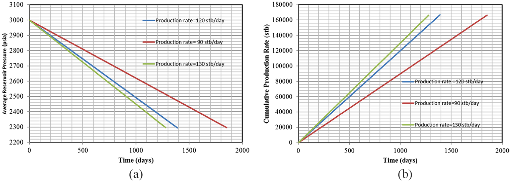
(a) Sensitivity impact of production rate on average reservoir pressure and (b) sensitivity impact of production rate on cumulative production.
Conclusion
In this article, a three-dimensional numerical reservoir simulator is developed for undersaturated reservoirs for an earliest possible determination and characterization of primary drive mechanisms. This objective is achieved by advancing simulation runs from initial reservoir conditions to future times by stepping through the simulation at discrete time steps to identify primary drive mechanism. The following conclusions were drawn from this current research.
This simulator combines volumetric, material balance, and reservoir simulation techniques to develop one complete robust tool for analyzing primary drive reservoirs.
The rates of average pressure decline and recovery factor estimations are the two main parameters to quickly identify the best-fit primary drive reservoir before bubble-point pressure is attained. Moreover, the best potential primary drive mechanism identified for this model is depletion drive reservoir or rock and liquid expansion drive.
Material balance error check (incremental (0.995) and cumulative (1.005)) is used to validate the numerical reservoir simulator developed in this research for its reliability and robustness for prediction and modeling of primary drive reservoirs until bubble-point pressure is attained. The error checks were within the acceptable tolerance limit.
FVF as a function of average reservoir pressure was not treated as a constant in the numerical simulator, but computed at each time step.
This numerical reservoir simulator developed in this study can be used to carry out reservoir simulation studies on full-field scale cases until saturation pressure to improve recovery efficiency in order to make strategic reservoir management decisions. Also, this numerical reservoir simulator can be used to validate simple analytical solution used in hydrocarbon recovery.
Sensitivity analyses can be performed on the numerical reservoir simulator developed in order to optimize reservoir parameters for efficient recovery under various operating conditions.
Crank–Nicolson scheme is unconditionally stable with no constraint on time step-size while preconditioned conjugate gradient iterative solver converges the numerical solutions faster.
Footnotes
Appendix 1
Acknowledgements
We would like to thank the anonymous reviewers for their comments and suggestions that were helpful in improving the manuscript.
Handling Editor: Dumitru Baleanu
Author’s note
Eric Thompson Brantson is now affiliated with Department of Petroleum Engineering, Faculty of Mineral Resources Technology, University of Mines and Technology, Tarkwa.
Declaration of conflicting interests
The author(s) declared no potential conflicts of interest with respect to the research, authorship, and/or publication of this article.
Funding
The author(s) disclosed receipt of the following financial support for the research, authorship, and/or publication of this article: This research was conducted partially with financial support from the China University of Geosciences Program under grant 2012026506 and with support from the faculty of earth resources of China University of Geosciences (Wuhan).